Variance Ranking for Multi-Classed Imbalanced Datasets: A Case Study of One-Versus-All

Abstract

Imbalanced classes in multi-classed datasets is one of the most salient hindrances to the accuracy and dependable results of predictive modeling. In predictions, there are always majority and minority classes, and in most cases it is difficult to capture the members of item belonging to the minority classes. This anomaly is traceable to the designs of the predictive algorithms because most algorithms do not factor in the unequal numbers of classes into their designs and implementations. The accuracy of most modeling processes is subjective to the ever-present consequences of the imbalanced classes. This paper employs the variance ranking technique to deal with the real-world class imbalance problem. We augmented this technique using one-versus-all re-coding of the multi-classed datasets. The proof-of-concept experimentation shows that our technique performs better when compared with the previous work done on capturing small class members in multi-classed datasets.

1. Introduction

When datasets are not equally group or divided, it is said to be imbalanced and most machine learning algorithms perform poorly on such datasets. Unfortunately, practically all real-world datasets are imbalanced. Learning from such imbalances has become the major obstacle to obtaining better predictive results. Most current research efforts are geared towards finding ways to minimize or totally eliminating the influence of the imbalance classes during predictive modeling. Though more research is being done by the day, some successful approaches, like the sampling techniques and their various modifications, have become state-of-the-art in learning from imbalanced data.

We now use data in every aspect of our life, from education to health, security, transportation, and beyond. This explosion in the data-driven economy was partly brought about by improvements in the available computational processing power, sensors, and associated radio-frequency identification (RFID) technology. The RFID could be used to tag any person, animal, or object, so as to collect data regarding the object’s movements and behavior [1]. There seems to be no limit to RFID technology; it has even been used intravenously on a living creature to study the internal environments of the organism for scientific and medical research.

The internet and the world wide web, some of the biggest inventions of our time, are the most fertile ground for harvesting raw data. The approaches to obtaining raw data are becoming easier by the day; it is a matter of developing a few lines of code in Python or any other programming language to scour the internet and obtain as much data as required on any topic.

The availability of data and its usage have led to the development of a specialized industry and group of highly skilled professionals called data scientists and machine learning experts. These skilled and knowledgeable “armchair scientists” have challenged the status quo in which scientists are known to work with samples and physical materials, slouching and peering over a microscope; in contrast, data scientists are only armed with raw data and predictive algorithms as the input and have made remarkable discoveries in almost all fields of human endeavor. Most recent inventions, such as driverless cars, voice intelligence, are within the scope of the expertise of these data scientists and allied professions.

However, the usage of these real-world data have shown some enduring and problematic patterns and inadequacy of the existing machine learning algorithm for dealing with the data or making better predictions due to this pattern. The pattern observed is that, in practically all real-world data, the classes are not equally divided [2], a phenomenon often called “imbalance”. There are two main types of imbalance. the first is binary class, which contains only two classes, for example, class 0/1, positive/negative, or yes/no. The other type is a multiple-class type, which contains more than two classes. 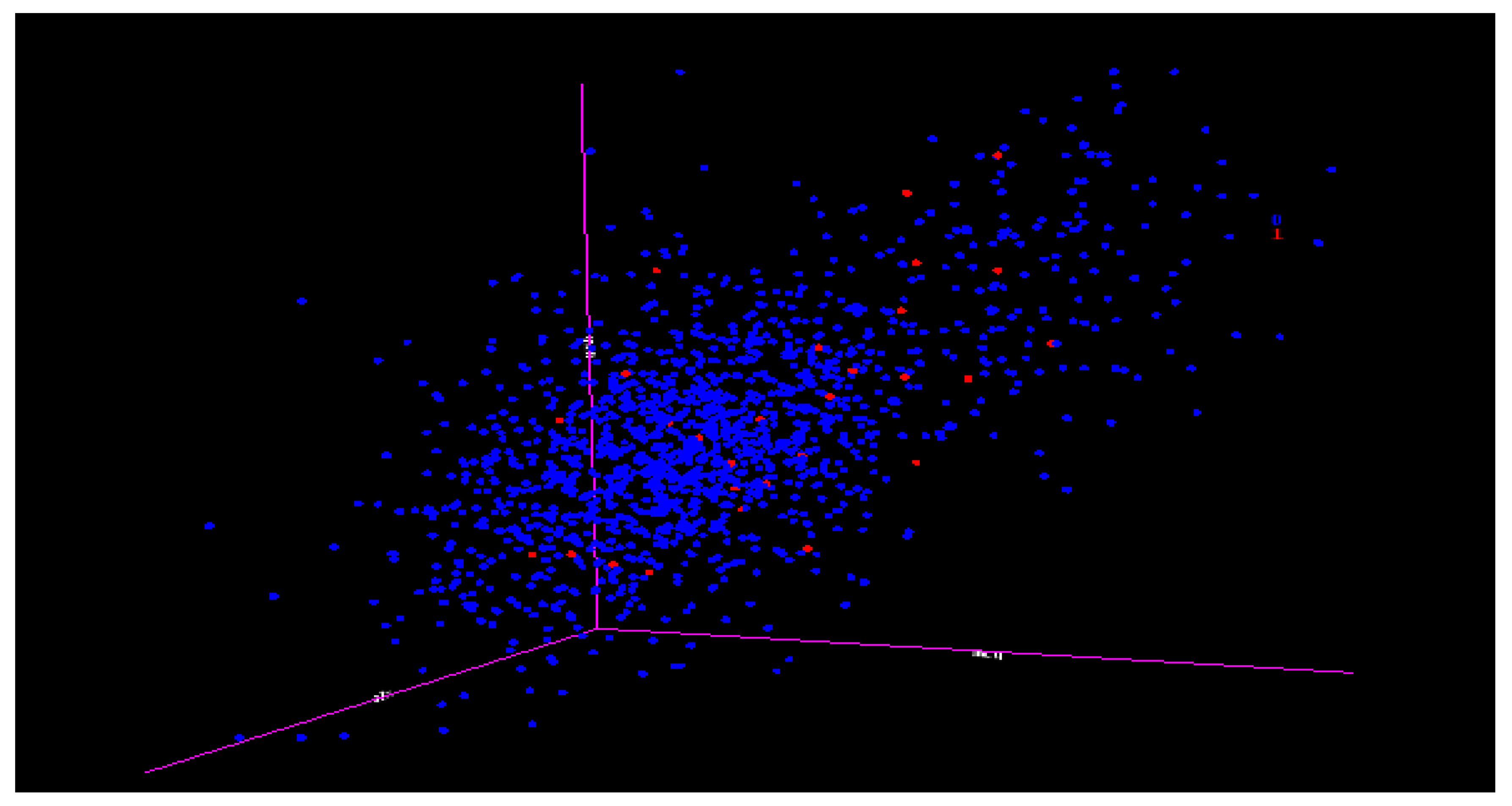Figure 1 provides a three-dimensional (3D) representation of the multi-class imbalanced data, where each color belongs to a different class. The issue that arises from this is that, in most predictive modeling, the smaller classes are less likely to be captured or picked up during the predictive modeling process. The smaller class group will be called the minority class, while the larger class group will be called the majority class.

Figure 1. Three-dimensional scattered plot of imbalanced data.

The accuracy of predictive modeling could be as high as 90% in binary class imbalanced data, whereas no minority class group has been captured; this is because the minority class has confused the algorithms and been misclassified, even if in most predictions, the minority classes are what is being sought. Therefore, the predictive modeling accuracy could be deceptive, representing a poor metric for measuring the performance of the predictions. The situation is even worse when there are multiple classes (more than two); here, some classes will appear to be practically non-existent in the modeling. Let us put multi-classed data into perspective by presenting a multi-classed scenario where imbalanced data could be obtained:

• Uncovering different global IP addresses where hacking attacks are coming to a computer server;
• Identifying different species of plants; and
• Identifying different types of glass, for example, window glass, tableware glass, car headlamp glass, and so on.

These are situations in which different classes of IP addresses, species of plants, or types of glasses are to be classified. All these and similar scenarios usually give rise to multi-class imbalanced data.

Quantitatively, the reason for the imbalanced class is known as imbalanced ratio (IR) [3,4,5]. The imbalance ratio is the ratio of the majority class to the minority class for imbalanced binary data in the population or ratios of all the classes for imbalanced multi-classed data in the population. Figure 2 presents imbalanced binary and multi-class data.

Figure 2. Imbalanced data.

In this paper, we present a novel approach for imbalanced learning. The main contributions of this paper are as follow;

• A novel variance ranking attribute selection technique that can augment one-versus-all to effectively handle imbalanced multi-class data.
• A system for selecting the most significant attributes by identifying the peak threshold performance for recall and accuracy; this will improve the selections of the most significant variable in a multi-class context.
• We presented a system of identifying and assessing the point at which a predictive modeling results will lose his dependability.

The remainder of the paper is organized as follows: Section 2 reviews all the related literature. In Section 3, we provide a review of the methodology with a clear theoretical base of variance ranking techniques, while Section 4 the re-coding of the multi-classed data using the one-versus-all approach was applied. Section 5 gives the experimental design of the variance ranking techniques, while Section 6 gives the comparison of the variance ranking and two state-of-the-art attributes selections. Section 7 presents the validation of variance ranking and Section 8 shows the comparison of variance ranking with two other techniques for solving issues of imbalanced data. finally Section 9 gives the conclusion and discusses future work.

2. Related Work

The general approaches for solving the problems of imbalanced classes could be categorized into three, these are the algorithm approach, the feature selection approach, and, finally, the sampling approach. We reviewed these approaches in the preceding sections.

2.1. The Algorithm Approach

This is, of course, the default approach used to solve the problems of imbalance in the data set. To put it in context, the reason predictive modeling is carried out is to be able to make a single or some specific decisions in a sea of other alternative options; therefore, other options are usually larger in number than the specific decision(s) we intend to make. This is a classic case of imbalance, where options are not evenly divided. All machine-learning algorithms were invented to aid in making these specific decisions. The right decisions being made are the basis of all successful human endeavor. Therefore, algorithms and data must be able to interact optimally to predict the right course of action when the need arises, but in reality, this is not the case because of the imbalanced classes in the data [6,7,8].

Researchers have always tried to minimize the effects of the class imbalance in predictive modeling by using different algorithms on datasets. For instance, [9,10] applied decision tree and to various samples of imbalanced data, while [11] used a weighted random forest algorithm. In the support vector machine categories of algorithms, the work of [12,13] demonstrated the efforts that have been made to solve the class imbalance by applying Support Vectors in sample space of datasets to create the demarcations between classes. Ref. [14] has applied the level of skewness to a multivariate dataset and implies that this relates to the distributions and ultimately the classes. Some researchers like [15,16] applied a deep learning algorithm to solve the imbalanced scenario of Malware detection. The real-world imbalance context being very ubiquitous has also been applied in mechanical failures, for example, [17] showed a situation that it could be used for locomotive fault detection and maintenance. Some have viewed the imbalanced class problems from the perspective of fuzziness, [18,19] hence used the concept to derive weighting values to rebalances and create synthetic minority data.

The question that arises is as follows: why are these algorithms that represent mature concepts and have stood the test of time performs poorly when the dataset is imbalanced [20]? The analysis of most of the machine learning algorithms provides some answers; initially, for once the algorithms did not factor in the unequal classes (imbalance ratio) in their designs and implementations, and many of the algorithms are optimized to recognize the dominant groups. For example, the kernel function in support vector machine (SVM) could easily detect the boundary of the dominant classes, and so on. This design by implications assumes that the classes are balanced because there is no quantity that accommodates variations in the number of classes in the formula of the algorithms [21]. Even if using a machine learning algorithm sometimes produces good results, but such results cannot be replicated when using different datasets from the same domain, for example, using different cancer data will not replicate the results obtained earlier because the intrinsic properties of the dataset differ from each other and require a lot of “tweaking” and “altering” parameters of algorithms. This is a normal practice in data mining and machine learning processes, but it means that the algorithm approach is not an exact science; instead, it is more in the realm of trial and error.

2.2. The Feature Selection Approach

Attribute or feature selection is not primarily intended to treat the issues of imbalanced classes. The reasons for supporting feature selection in data-centric research include avoiding overfitting, lengthy training time, and resource issues. Imagine obtaining approximately the same level of accuracy by using only five selected features instead of a total of 10 features in a data mining process, considering the time and other resources it may take to acquire all the 10 features and many of them may not be necessary to the prediction. Of course, feature selection improves the accuracy of classifiers and invariably enhances the capture of the minority in a dataset, along with several advantages.

Feature selection is categorized into two basic groups, namely, the filter and wrapper techniques; some hybrid techniques that are combinations of these two categories are also available. The filter techniques is algorithm independent, while the wrapper approach is algorithm dependent. There are various filter techniques; as shown in Table 1, each of them uses different or combinations of statistical functions like distance, correlation, information metric and similarities as a means of ranking the feature relevance in the dataset. Although filter techniques are algorithm independent not all filters can be used for all types of predictive modeling: some are more suited for a different type of modeling like classification, regression, and clustering.

Table 1. Common filter feature selection techniques.

Common Filter Technique For Feature Selection
Name	Suitable	Basic Metric
Information Gain	Classification and Regression	Entropy
Pearson Correlation	Classification and Regression	Correlation
Gini Ratio/Gini Index	Classification and Regression	measure of statistical dispersion
Fischer Score	Classification and Regression	distance between data points
Chi-square	Classification and Regression	dependency of two variables
Others	Classification and Regression and Others	Others

Wrapper techniques are algorithm dependent; here a predetermined algorithm used in the modeling is known or the technique recommends which algorithm is most suitable for the selected feature. Hence, a subset of the overall features in the dataset is created, which should comprise the features deemed most important for a specific classifier performance.

More often than not, not all the features are included in the subset, as some are eliminated. The subsets are combinations of various features based on some black-box search algorithms called “attribute evaluator”. Some of the most common wrapper techniques are “CfsSubsetEval”, “ClassifierSubsetEval” and “WrapperSubsetEval”.

Feature or attributes selection is an active area of research related to solving the issues associated with imbalanced data classes; apart from those listed in Table 1 many researchers have recently delved into solving this problem; notably [22] proposed four metrics information gain (IG), chi-square (CHI), correlation coefficient (CC), and odds ratios (OR) the most effective way of selecting the features in a datasets. Although the results of these recommendations were encouraging, but failed when the four metrics did not triangulate or come together. This made the validity of the work conditional based on only three methods triangulating. Another notable work is that of [23] which uses the receiver operating characteristics (ROC) to imply that the significant features could be obtained using a technique called “feature assessment by sliding thresholds” (FAST)”, but the ROC is a “what-if” conditional probability simulations scenario, and in reality, such a condition may not arise. The work of [24] uses adaptations of the ensemble (combinations) of multiple classifiers based on feature selection, re-sampling, and algorithm learning. In line with using ensemble approaches to feature selections, a method called MIEE (mutual information-based feature selection for EasyEnsemble) was proposed by [25]. Moreover, a comparison was shown with other ensemble methods, such as asymmetric bagging, which the EasyEnsemble performs better. A technique called K-OFSD, which combines K nearest neighbors and its dependency on rough set theory for selecting features in high-dimensionality datasets was invented by [26]. Feature selection and imbalanced data is an active area of research, and new effort will continue to be made to find solutions to both.

2.3. The Sampling Approach

There are two categories of sampling; oversampling and undersampling. Oversampling increases the amount of minority data, while undersampling reduces it. We concentrated on oversampling approaches; prominent among them is the first to be invented, which was a synthetic minority oversampling technique (SMOTE). This was invented by [27], and it was the first meaningful technique for solving the imbalanced issue. A few years of adaptive synthetic sampling (ADASYN) was invented by [28]. Over the years, different modifications of oversampling techniques like the BorderlineSMOTE and SMOTETomek have continued to be invented. Though oversampling methods could produce very good results when the datasets are not overlapped, but performed poorly with overlapped datasets, this led to implementations of weighting oversampling like the majority weighted minority oversampling technique (MWMOTE) by [29] where the minority classes that are difficult to learn are identified and assigned a weight.

What is the reason for the imbalance? It is due to the unequal numbers of classes and is called IR. Any technique, formula, or algorithm that does not factor in the IR will always produce unreliable and inconsistent results when trying to replicate the experiments using different data.

Apart from sampling techniques like SMOTE, ADASYN and other modifications of sampling techniques. Variance ranking (VR) attributes selection is the only technique that has factored the IR in for dealing with imbalanced class problems. To summarize what SMOTE and ADASYN does, they artificially generating data items for minority classes using different techniques to make all the class groups equal (making the IR 1:1), meaning that there are equal numbers of both the majority and minority classes. Since SMOTE and ADASYN use the IR like our approach (VR), the three are compared in later sections.

3. Overview of Research Methodology

This section is divided into two categories. Firstly, the strategy of Variance Ranking and how it will be implemented in the research design using the variances and variable properties will be derived. Secondly, the techniques of decomposing multi-classed data into n binary using the concepts of “one-versus-all” and “one-versus-one”. This decomposition augment the variance ranking techniques. Finally, the review of classification measurement metrics, re-coding of the multi-classed datasets will be demonstrated.

3.1. Methodology for Variable Properties Derivatives

All classes of data that share the same vector space are subjected to the same constant density known as probability density functions, but the probability stems from the fact that for each data sample, the value of the density function is a likelihood of being equal to the sample at the same point. Therefore since density is inversely proportional to variances, the comparison of the variances in a sample space would show the density of each group and their classes. Suppose we want to find the differences among this group of data, which have been divided into subsets; class 1 and class 0 as explained in Section 5. We have a statistical means of doing this called analysis of variance (ANOVA) [30]. Based on the comparison, we can now represent multivariate ANOVA as in the Equation (1)

$$CompareRatio=\frac{Varianc{e}_{\left(class1\right)}}{Varianc{e}_{\left(class2\right)}}.$$

(1)

The ratio of two random variable events can now be a metric to compare their degree of concentrations in a sample space where it is equal to the probability functions [31], agreeing with Equation (1).

Thus, the ratio of the variance of each variable in the majority and minority data subsets is proportional to the density functions, while the square of the density function is equal to the F-distribution. The F-distribution deals with multiple set of events or variables as represented in form of different variables in the majority and minority data classes. By definition, the F-distribution (F-test) [32] is represented by the formula

$$F=\frac{{\left(Largervariance\right)}^2}{{\left(smallervariance\right)}^2}.$$

(2)

Therefore, a subset (class 1 and 0) with additive variance independent variable will resolve into

$$F_{final}={\left\{\frac{Varianc{e}_{\left(final1\right)}}{Varianc{e}_{\left(final2\right)}}\right\}}^2.$$

(3)

Here, unit of $F_{final}$ is the same unit as the variance; therefore, $F_{final}$ is a measure of variance of the variances $Varianc{e}_{\left(final1\right)}$ and $Varianc{e}_{\left(final2\right)}$. For binary data or multi-class data decomposed into binary using a one-versus-all set, if the subclass variance is $V_i$ and $V_j$, then the Equation (3) would resolve to Equation (4), the squaring is both a mathematical expediency to eliminate negative value and also agrees with the F-distribution (F-test); finally, the value of (F-test) is $F_{final}$

$$F_{final}={\left[\frac{V_{0j}}{V_{1j}}\right]}^2.$$

(4)

3.2. Variance Ranking Methodology

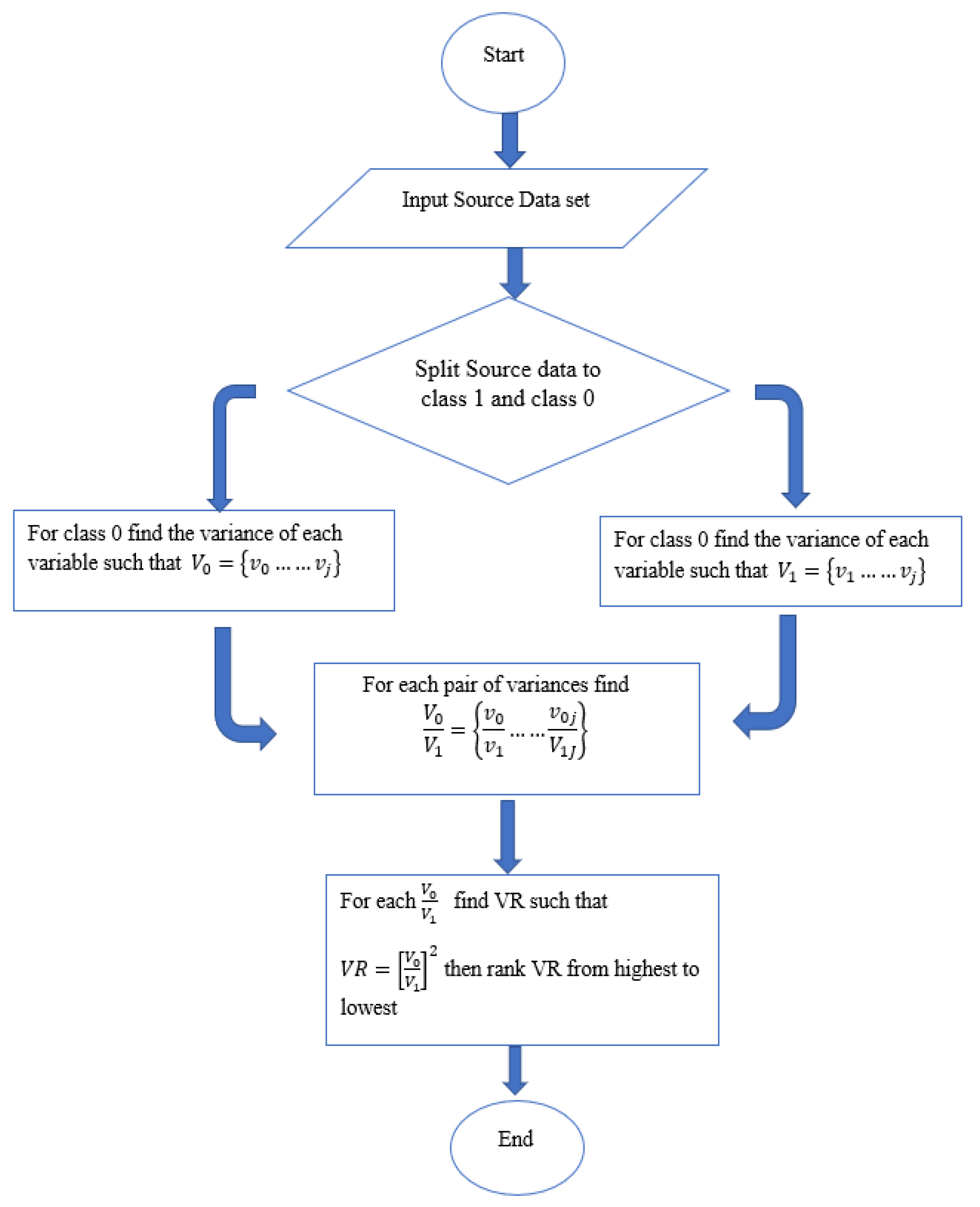
The steps of variance ranking methodology are depicted in the algorithm in Figure 3. A typical real-world dataset is made of a series of attributes (variables). Let the variance of each of these variables be represented by V = V₀, …..V_j if an input training data set with N number of variables are split into two groups of class 1 and class 0. Therefore for each of the classes (class 1 and class 0) the variables V become $V_1$ and $V_0$ respectively. It follows that the variances of $V_1$ and $V_0$ are represented by v₁ = v₁, …..v_j and v₀ = v₀, …..v_j being the variances of each of the variables (attributes) for their respective classes.

Figure 3. Algorithm flow chart for variance ranking attribute selection.

Considering the concentrations of each variable in the sample space, which are equal to the density of the variable in the same space. The ratio of the pair of variances of the variable classes (F-distribution) could be used to determine this concentration as in Equation (4). Hence applying the $V_1$ and $V_0$ to Equation (4) for each pair of variance will give finally ${\left\{\frac{v_0,.....v_j}{v_1,.....v_j}\right\}}^2$, ranking the results from highest to lowest is the is the variance ranking (VR). please see Figure 3 for visual representation of these processes.

3.3. Methodology of Decomposing Multi-Classed into n Binary

The measure of classifier performance in imbalanced binary datasets is straightforward and easily understandable, but for multi-class cases, misclassified and overlapping data make it impossible to effectively measure performance, one of the most useful techniques is decomposing the classes into series of $n_{total}$ binary classes where n is the number of classes [33].

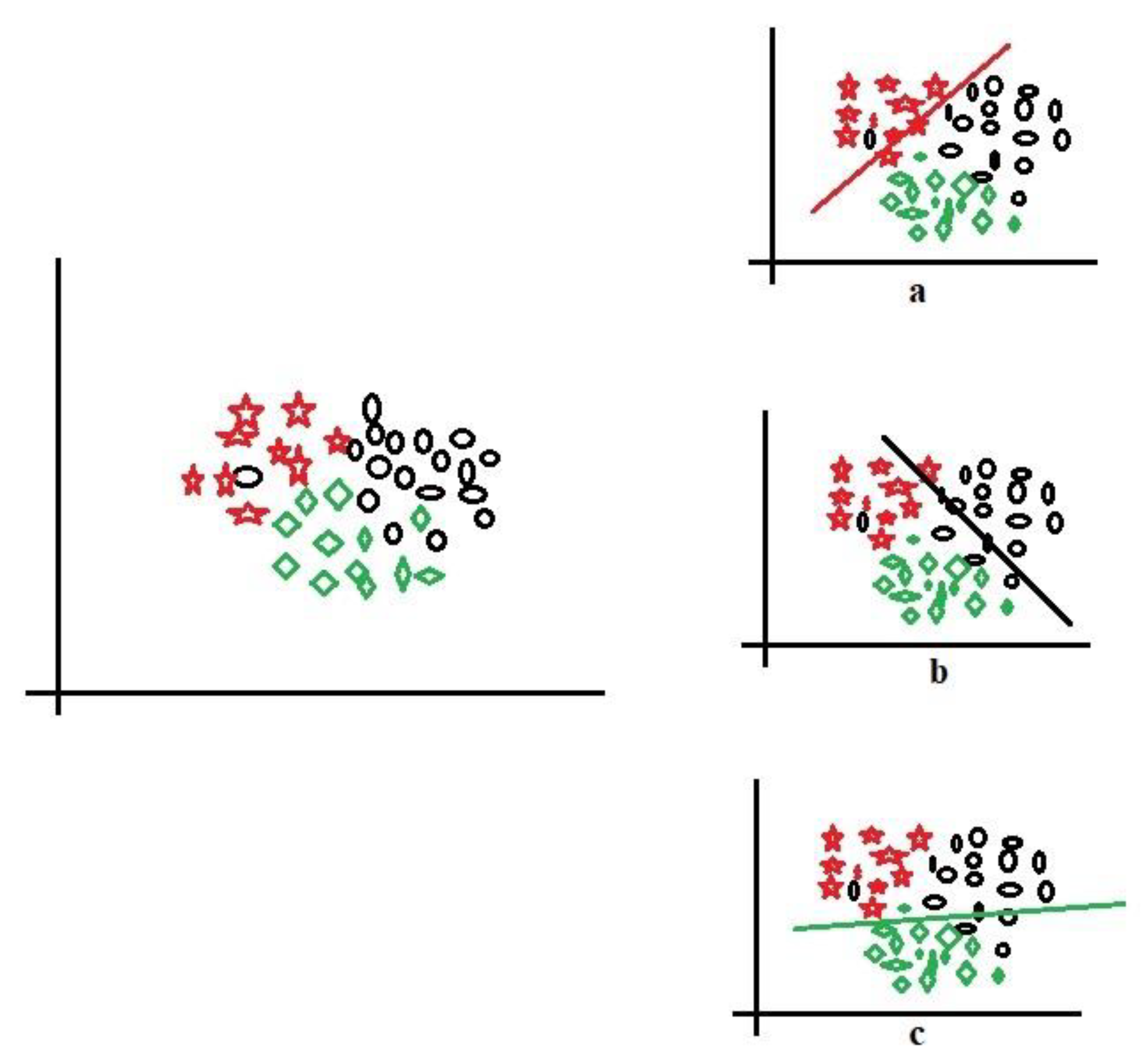
For clarity, Figure 4 shows three-class data represented by red stars, black circle, and green squares for implementing the one-versus-all technique. Let us take the red stars as the positive class (Figure 4a), demarcated by the red line; the other components (black circles and green squares) are the negative class. Sequentially, the black circles (Figure 4b) and green squares (Figure 4c) are taken in turn to be positive while the rest are negative; this is the process of decomposing multiple classes into (n) binary. With this decomposition, the binary performance evaluations in Section 3.4 could be applied to evaluate the multi-class data. The one-versus-all could also be called one-versus-rest and is one of the most popular and accurate methods for handling multi-class datasets.

Figure 4. Multi-class to binary decomposition: one-versus-all. (a): consider the red stars as a positive class and the rest are negative; (b): consider the black circles as a positive class and the rest are negative; (c): consider the green squares as a positive class and the rest are negative.

Another way for handling multiple classes is one-versus-one techniques; this process takes each pair of classes in the multi-class dataset in turn, until all the classes have been paired with each other.

Figure 5 shows one-versus-one for multi-class dataset, where each class is paired with another until all the classes have been paired. For example, classes 2 and 3 are paired in Figure 5a, classes 1 and 2 in Figure 5b, and finally, classes 1 and 3 in Figure 5c.

Figure 5. Multi-class binary decomposition: one-versus-one. (a): Classes 2 and 3 are paired; (b): Classes 1 and 2 are paired; (c): Classes 1 and 3 are paired.

There is extensive literature that has proposed and supported one-versus-all techniques as the most accurate approach for handling multi-class classifications; the work of [34] made a strong case for this technique as the only techniques that could justifiably claimed to have actually handle multiclass classification in a real sense of it, because one-versus-one makes a pair of binary data without accounting for the influence of other data items, meaning that other data items that could interact with the modeling have been eliminated or filtered out. In contrast, in one-versus-all, those classes have not been removed. Furthermore, one-versus-one is computationally expensive. Hence, the one-versus-all approach is implemented in this work.

3.4. Measurement Evaluation of Classifications

Having decomposed the multi-classed into binary data using one-versus-all, the metric of measuring the binary classification can be applied to evaluate the experiments. The binary classification evaluation experiment is represented by a 2 × 2 confusion matrix, as shown in Table 2. This is particularly useful for visualizing a binary classification against a multi-class classification, where multiple overlappings of classification could confuse the algorithms and make the results; less discriminant; a detailed analysis of the confusion matrix can be found in [35]. The terms definition in confusion matrix table are

Table 2. Confusion matrix.

	Predicted
	Positive	Negative
Actual Yes	TP	FN
Actual No	FP	TN

• True positive (TP): The algorithm predicted yes, and the correct answer is yes; (correctly predicted);
• True negative (TN): The algorithm predicted no, while the correct answer is no (predicted correctly);
• False positive (FP): The algorithm predicted yes, while the correct answer is no (incorrectly predicted); and
• False negative (FN): The algorithm predicted no, but the correct answer is yes (incorrectly predicted).

The true positive rate (TPR) is the same as the sensitivity and recall. It is the proportion of positive values that are correctly predicted:

$$Sensitivity=Recall=\frac{TP}{(TP+FN)}.$$

(5)

The precision is the proportion of predicted positives that are truly positive:

$$Precision=\frac{TP}{(TP+FP)}.$$

(6)

Specificity is the proportion of actual negative that are predicted to be negative

$$FP\left(rate\right)=Specificity=\frac{TN}{(TN+FP)}.$$

(7)

The F-measure is the harmonic mean between precision and recall or the harmonic mean between specificity and sensitivity:

$$F_{measure}=2\ast \frac{Precision·Recall}{(Precision+Recall)}.$$

(8)

$$Accuracy=\frac{tp+tn}{(tp+tn+fp+fn)}=\frac{tp+tn}{n}.$$

(9)

The F-Measure can also assess the performance of the predictions [36] as another metric that has been indicated from Equations (5)–(9). The metric to use depends on what the researcher is trying accomplish.

4. Dataset and One-Versus-All Re-Coding

The datasets used in the experiments are Glass data and Yeast data; these two datasets are highly multi-classed, and they have been converted to n Binary using the one-versus-all techniques as explained in Section 3.3; hence, the same data metric of measurement in Section 3.4 could be applied to validate the experiments. The next sections will demonstrate the re-coding of the Yeast and Glass data sets.

4.1. The Re-Coding of the Glass and the Yeast Datasets Using One-Versus-All

The Glass data set has $n=6$ classes. The imbalanced classes are from 1 to 7; notice that class 4 is not in this dataset, so the total number of available classes is six, and they are originally labeled as classes 1–3 and 5–7. Using the “one-versus-all” process, as explained in Section 4 each of these classes will be taken in turn as class 1 (minority class) and the others as class 0 (majority class).

The Glass data imbalanced contents proportion is shown in Figure 6, which represents the type of class based on the chemical elements compositions and the refractive index (RI). The refractive index is a physical property of glass that measures the bending of light as it passes through.

Figure 6. Glass data contents proportion.

The amount of the chemical compositions of a glass determines its application, type, and classes; for example, class 1 is “building window float processed”, class 2 is the “building window non-float processed”, class 3 is “vehicle window float processed”, class 4 (not available in this dataset) is “vehicle window known-float processed”, class 5 is “container”, class 6 is “tableware”, and finally, class 7 is “headlamps”. Therefore, the experiment will be conducted with class 1 as the minority while the rest will be class 0 as the majority class. Each of the classes in the minority, as shown in Figure 6, will consequently be relabel as class 1 and class 0. Table 3 is the implementation of the one-versus-all approach; it shows the relabeled table with the actual numbers of minority classes as 70, 76, 17, 13, 9 and 29 and the corresponding majority classes are 144, 138, 197, 201, 205 and 185.

Table 3. Glass data class relabel in One versus All.

Original Class Label	Number	Minority (One)	Majority (All)
1	70	70 class 1	144 class 0
2	76	76 class 1	138 class 0
3	17	17 class 1	197 class 0
4	Unavailable	Unavailable	Unavailable
5	13	13 class 1	201 class 0
6	9	9 class 1	205 class 0
7	29	29 class 1	185 class 0

For the Yeast data, the imbalanced classes can be seen in Table 4 and the content proportions in Figure 7. This dataset is one of the most popular ones, and it has been used in various work for imbalanced multi-class data. The data are numeric measurements of different proteins in the nucleus and cell materials in Yeast unicellular organisms. The objective of the dataset is using this physical protein descriptor for ascertaining the localization, which in turn, may provide help explaining the growth, health, and other physical and chemical properties of Yeast. The data are made up of 1484 instances. The final result of using the VR techniques for the glass dataset is shown in Table 5 again, notice that the serial numbers of each element as ranked by the experiment. Each of the sub-tables in Table 5 is a representation of each class relabelled as class 1 and the rest as class 0; for example, class 2 is relabelled as class 1 and the rest as class 0, (one-versus-all). This process is continued for all the classes in the dataset; see Table 3. The re-coding of the dataset to one-versus-all is shown in Table 4. For example, the recoding proceeds as “CYT (463) as class 1, 1023 as class 0”; this continues until the last minority class, which is “ERL(5) as class 1, 1481 as class 0.

Table 4. Yeast data class relabeling to one-versus-all.

Original Class Label	Number	Minority (One)	Majority (All)
CYT (cytosolic or cytoskeletal)	463	CYT 463 as class 1	1023 as class 0
NUC (nuclear)	429	NUC 429 as class 1	1057 as class 0
MIT (mitochondrial)	244	MIT 244 as class 1	1242 as class 0
ME3 (membrane protein, no N-terminal signal)	163	ME3 163 as class 1	1323 as class 0
ME2 (membrane protein, uncleaved signal)	51	ME2 51 as class 1	1435 as class 0
ME1 (membrane protein, cleaved signal)	44	ME1 44 as class 1	1442 as class 0
EXC (extracellular)	37	EXC 37 as class 1	1449 as class 0
VAC (vacuolar)	30	VAC 30 as class 1	1456 as class 0
POX (peroxisomal)	20	POX 20 as class 1	1466 as class 0
ERL (endoplasmic reticulum lumen)	5	ERL 5 as class 1	1481 as class 0

Figure 7. Yeast data contents proportion.

Table 5. Experiment on Glass data.

sn	Variables	V0	V1	VR	sn	Variables	V0	V1	VR	sn	Variables	V0	V1	VR
8	Ba	0.345686	0.007029	2418.831	6	K	0.425354	0.045679	86.71029	8	Ba	0.247227	0.001324	34891.9
3	Mg	2.521579	0.06103	1707.084	4	Al	0.24927	0.101341	6.05026	3	Mg	2.08054	0.026499	6164.313
6	K	0.609499	0.046173	174.2486	8	Ba	0.247227	0.131291	3.545884	7	Ca	2.025366	0.144485	196.5007
7	Ca	2.838831	0.330403	73.82303	2	Na	0.666841	0.441108	2.285366	6	K	0.425354	0.052849	64.77741
4	Al	0.277826	0.074615	13.86399	3	Mg	2.08054	1.477833	1.981991	2	Na	0.666841	0.256935	6.735968
2	Na	0.853034	0.249302	11.70795	5	Si	0.599921	0.525005	1.305753	1	RI	9.22 × 10−6	3.67 × 10−6	6.306561
5	Si	0.736367	0.324312	5.155397	9	Fe	0.009494	0.011328	0.702465	5	Si	0.599921	0.262426	5.226045
1	RI	1.12 × 10−5	5.14 × 10−6	4.709949	1	RI	9.22 × 10−6	1.45 × 10−5	0.407001	4	Al	0.24927	0.120749	4.261642
9	Fe	0.010313	0.007934	1.689589	7	Ca	2.025366	3.692682	0.300831	9	Fe	0.009494	0.011635	0.665926
Class 1= relabelled as class 1, others class 0					Class 2= relabel as class 1, others class 0					Class 3 is relabelled as class 1, others class 0
sn	Variables	V0	V1	VR	sn	Variables	V0	V1	VR	sn	Variables	V0	V1	VR
3	Mg	2.08054	0.998292	4.34347	3	Mg	2.08054	1.203703	2.98754	9	Fe	0.01051	0.000888	140.1712
2	Na	0.666841	0.603786	1.219773	7	Ca	2.025366	2.10235	0.928105	7	Ca	2.160844	0.947712	5.198688
1	RI	9.22 × 10−6	1.12 × 10−5	0.679098	1	RI	9.22 × 10−6	9.71 × 10−6	0.902469	1	RI	9.41 × 10−6	6.48 × 10−6	2.10864
8	Ba	0.247227	0.369969	0.44654	4	Al	0.24927	0.327025	0.581003	3	Mg	1.378535	1.249215	1.217759
4	Al	0.24927	0.481526	0.26798	2	Na	0.666841	1.1751	0.322029	2	Na	0.505249	0.471088	1.150284
7	Ca	2.025366	4.768942	0.180369	5	Si	0.599921	1.16525	0.265064	6	K	0.419003	0.446883	0.879119
9	Fe	0.009494	0.024208	0.153822	6	K	0.425354	0	0	4	Al	0.17496	0.196006	0.796774
5	Si	0.599921	1.644342	0.133108	8	Ba	0.247227	0	0	5	Si	0.541864	0.884039	0.375697
6	K	0.425354	4.574017	0.008648	9	Fe	0.009494	0	0	8	Ba	0.08243	0.442679	0.034673
Class 5 is relabelled as class 1, others class 0					Class 6 is relabelled as class 1, others class 0					Class 7 is relabelled as class 1, others class 0

5. Research Design Experiment to Demonstrate Variance Ranking

In this section all the experiments carried out to demonstrate variance ranking attribute selection using the Yeast and Glass datasets will be shown. This section will be a follow up of the previous Section 4, where the datasets have been re-coded from multi-classed to n binary using the one-versus-all approach. The sequence of the experiments is as follows.

• each of the two (Yeast and Glass) datasets that have been recorded were split into class 0 (minority) and class 1 (majority);
• The variances, $V_0$ and $V_1$ of each of the attributes in class 0 and class 1 is calculated, such that V₀ = v₀₁……v_0j and V₁ = v₁₁……v_1j;
• For each of the calculated variance of the class attributes, we deduce the density distribution by finding the square of the ratio of $V_0$ to $V_1$.
• Ranking the ratio of square of $V_0$ to $V_1$ from highest to lowest would provide the most significant attributes that belong to each of the classes.

The proposed method of attribute selections is for continuous and discrete numeric data for a binary class and multi-class (decomposed into $n\mathrm{binary}$; see Section 3.3) provided that each attribute split is within the same range, meaning that they share a common denominator which is the same vector space.

In general, the variance of the subsections class 1 and class 0, of dataset was computed using the following formula Variance $v=\frac{\sum (x-{\overline{x}}^2)}{(n-1)}$. If the variance of the subsection of class 0 is given by:

$$V_0=\frac{(x_0-{\overline{x_0}}^2)}{(n_{maj}-1)},$$

(10)

and the variance of the subsection of class 1 is given by:

$$V_1=\frac{(x_1-{\overline{x_1}}^2)}{(n_{min}-1)},$$

(11)

the variance comparison is deduced by

$$VR={\left(\frac{(x_0-{\overline{x_0}}^2)}{(n_{maj}-1)}/\frac{(x_1-{\overline{x_1}}^2)}{(n_{min}-1)}\right)}^2={\left\{\frac{V_0}{V_1}\right\}}^2.$$

(12)

The total number of data items is inversely proportional to the variance or spread from the mean position, that is $Variance\propto \frac{1}{n_m}$; this relationship shows that the formula is generic, and therefore, if the ranking is done in either order, it will remain consistent. In Table 5, the columns $V_1$ and $V_0$ are the results of the variance of each subsection class 1 as the positive and class 0 as the negative for each attribute. The column $(V_0/V_1)$ is the division ratio based on the variance significant F-distribution given by ${\left\{\frac{V_0}{V_1}\right\}}^2$ to produce a value that could be squared.

The details of the dataset were explained in Section 4.1, and the technique of one-versus-all re-coding in Section 4. The total number of samples used in the experiments makes no difference provided the numbers of majority class and the minority class is maintained. You could even split before taking sample or take the sample before splitting provided the number of class 0 and class 1 are maintained proportionally, the values of the variances will remain the same with very low margin of differences.

The variance of each attribute was deduced using Equations (10) and (11). The significant variance is deduced using Equation (12). The total numbers of the majority and minority classes are maintained through the number of the data items as $n_{maj}$ and $n_{min}$. The first sub-table in Table 5 is class 1, and the rest classes combine (class 2, 3, 5, 6 and 7; notice no class 4) are class 0. The VR technique ranks the most significant attributes as follows Ba, Mg, K and so forth. The second experiment has class 2 re-labeled as class 1 and the other classes (1, 3, 5–7) combined as class 0; this ranked K, Al, Ba, and so on, as the most significant. The next experiment is class 3 relabeled as class 1 while the rest as class 0; this ranked Ba, Mg, Ca, and so on. All six classes are taken in turn.

The general postulate here from the experimental result is that the type of glass depends on the amount of chemical element that the glass contains; this has been captured by the VR technique.

6. Comparing Variance Ranking with Pearson Correlation (PC) and Information Gain (IG) Feature Selections

Most feature selection results are heuristics [37], meaning that no two feature selection on the same dataset will produce the same result perfectly, especially in the filter algorithm; instead, each attribute identified are most likely to be ranked slightly differently by different filter feature selection algorithms. To estimate or measure the similarities in these results, the order of ranking of the attributes becomes the metric used to quantify the similarities. Some of the identified attributes may be in the same position in the order of ranking, while others may share similarities by proximity to the attribute’s positions. The results obtained in Table 5 and Table 6 will be paired with the result of Pearson correlation (PC) and information gain (IG) attribute selection on the same data to investigate the extent of their similarities and differences.

Table 6. Experiment on Yeast data.

Variable	V0	V1	VR	Variable	V0	V1	VR	Variable	V0	V1	VR
vac	0.003343336	0.00043	60.45474339	nuc	0.011507	0.002703	18.12226	nuc	0.011446	0.001909	35.93054
nuc	0.011370412	0.00188	36.57941315	mit	0.01893	0.008878	4.546297	mit	0.00758	0.002582	8.620148
mcg	0.018614135	0.00427	19.00334227	vac	0.003348	0.002433	1.893481	vac	0.003365	0.001622	4.303174
mit	0.011882836	0.00443	18.06414534	mcg	0.018795	0.019936	0.888812	mcg	0.01889	0.012346	2.344098
alm	0.007513117	0.00847	0.78681652	alm	0.007472	0.008474	0.777556	alm	0.015399	0.012891	1.427042
gvh	0.015108362	0.01832	0.680117288	gvh	0.015301	0.017983	0.723933	gvh	0.018872	0.017736	1.132282
erl	0.001513064	0	0	erl	0.002386	0	0	erl	0.00128	0.163845	6.11 × 10−5
pox	0.005747052	0	0	pox	0.005845	0	0	pox	0.002369	0	0
ERL as class 1, others as class 0				VAC as class 1, others as class 0				POX as class 1, others as class 0
Variable	V0	V1	VR	Variable	V0	V1	VR	Variable	V0	V1	VR
vac	0.011544262	0.0003879	885.7163556	mcg	0.01667	0.004505	13.6918	nuc	0.011616	0.002673	18.88129
nuc	0.019108645	0.00502235	14.47589106	gvh	0.013591	0.005372	6.400738	alm	0.007313	0.005705	1.642763
mcg	0.007621846	0.00298437	6.522515713	alm	0.007151	0.003564	4.026557	mit	0.018899	0.015743	1.441004
mit	0.017648872	0.01223143	2.081994308	nuc	0.011446	0.007987	2.053653	gvh	0.015005	0.014494	1.071998
alm	0.014292326	0.0115516	1.530811824	mit	0.018805	0.016206	1.34654	vac	0.003327	0.003686	0.814611
gvh	0.003257518	0.00491345	0.43954295	vac	0.003326	0.003714	0.801938	mcg	0.016816	0.025717	0.427544
erl	0.002393773	0	0	erl	0.002409	0	0	erl	0.002249	0.004902	0.210487
pox	0.005864923	0	0	pox	0.005901	0	0	pox	0.00593	0	0
EXC as class 1, others as class 0				ME1 as class 1, others as class 0				ME2 as class 1, others as class 0

The VR, PC, and IG are given by:

$$VR={\left(\frac{(x_0-{\overline{x_0}}^2)}{(n_{maj}-1)}/\frac{(x_1-{\overline{x_1}}^2)}{(n_{min}-1)}\right)}^2={\left\{\frac{V_0}{V_1}\right\}}^2.$$

(13)

$$PC=\frac{\sum (x-\overline{x})(y-\overline{y})}{\sum {(x-\overline{x})}^2\sum {(y-\overline{y})}^2}.$$

(14)

$$IG=Entrop{y}_{\left(x\right)}-Entrop{y}_{(x,y)}.$$

(15)

Table 7 is the presentation of the results of the comparison of VR, PC, and IG feature selection techniques on the highly imbalanced Glass data. Originally, the Glass dataset is made up of six classes labeled class 1–3, 5–7 (notice there is no class 4), each of the smaller tables in Table 7 is a representation of these classes’ results. To carry out the “one-versus-all” experiment explained in the previous sections and Table 3, each class was relabelled in turn as class 1 and others combined as class 0. In the first smaller table in Table 7 (class 1 labeled as 1 and the others as 0), the VR and PC identifies Ba, Mg, and K in the first rows; the sixth and ninth rows have the same results. The IG and VR are not far off from each other; the fourth and fifth rows identify Al, while the eighth and ninth rows identify Fe. Although there are no rows that identify the same elements, the closeness is greater between VR and IG than it is between PC and IG; for this first experiment, in Table 7, VR and IG are more similar. The quantitative weighting of the similarities in these three feature selection algorithms will be calculated in Section 6.1 using the ROS technique.

Table 7. Comparison of variance ranking (VR) with Pearson correlation (PC) and information gain (IG) variable selection for Glass data.

Ranking of variable based on different feature selection Algorithms			Ranking of variable based on different feature selection Algorithms			Ranking of variable based on different feature selection Algorithms
Variance Ranking	Pearson Correlation	Information Gain	Variance Ranking	Pearson Correlation	Information Gain	Variance Ranking	Pearson Correlation	Information Gain
Ba	Ba	Ri	K	Ba	Ri	Ba	Ba	Ri
Mg	Mg	Na	Al	Fe	Ca	Mg	Mg	Si
K	K	Ca	Ba	K	Na	Ca	K	Na
Ca	Al	Al	Na	Mg	Si	K	Na	Ca
Al	RI	Si	Mg	Ri	Al	Na	Al	Al
Na	Na	Mg	Si	Al	Mg	RI	Ca	Mg
Si	Ca	K	Fe	Ca	K	Si	Si	K
RI	Si	Fe	RI	Na	Fe	Al	Ri	Fe
Fe	Fe	Ba	Ca	Si	Ba	Fe	Fe	Ba
Class 1 = labelled 1, others class 0			Class 2= relabelled as class 1, others class 0			Class 3 is relabelled as class 1, others class 0
Ranking of variable based on different feature selection Algorithms			Ranking of variable based on different feature selection Algorithms			Ranking of variable based on different feature selection Algorithms
Variance Ranking	Pearson Correlation	Information Gain	Variance Ranking	Pearson Correlation	Information Gain	Variance Ranking	Pearson Correlation	Information Gain
Mg	Fe	Ca	Mg	Fe	Na	Fe	Ba	Ri
Na	Mg	Ri	Ca	K	Ca	Ca	Mg	Na
RI	K	Al	RI	Ba	Ri	RI	K	Al
Ba	Al	Si	Al	Mg	Si	Mg	Fe	Ba
Al	Si	K	Na	Al	Mg	Na	Na	Ca
Ca	Na	Na	Si	Si	Al	K	Al	Si
Fe	Ca	Mg	K	Na	k	Al	Ca	K
Si	Ri	Fe	Ba	Ca	Fe	Si	Si	Mg
K	Ba	Ba	Fe	Ri	Ba	Ba	Ri	Fe
Class 5 is relabelled as class 1, others class 0			Class 6 is relabelled as class 1, others class 0			Class 7 is relabelled as class 1, others class 0

In the second experiment (class 2 relabeled as class 1 and the others as 0), none of the three feature selections ranked any of the elements in the same row, but proximity between rows elements is higher for VR and PC in row one and row three identifying Ba and K, in rows fourth and fifth, Mg is identified, as well as in many other rows. Similar proximity in the elements identified are also noticeable throughout between VR and IG, but the reversal of ranking of identified elements between PC and IG is also noted.

In the third smaller table in Table 7 (class 3 re-labeled as class 1 and the others as class 0), rows one, two, seven, and nine are the same in VR and PC and many other rows have proximity similarities; for example, rows three and four identify K, rows fourth and fifth identifies Na.

In the fourth small table in Table 7 (class 5 re-labeled as class 1 and the others as class 0), the VR does not have any row in common with PC and IG. However, close proximity is noticed in rows one and two for element Mg, rows five and four for element Al, and rows sixth and seventh for elements Ca for VR, PC, and IG share rows sixth and ninth in common and other rows as proximity.

In the fifth smaller table in Table 7 (class 6 re-labeled as class 1 and the others as class 0), VR and IG are more similar; in the second and sixth rows while the other rows are similar by proximity. In the final experiment is (class 7 re-labeled as class 1 and the others as class 0), the VR and PC are more similar because row five and eight, which have Na and Si, respectively.

For the Yeast dataset, the comparisons are given in Table 8, which are both divided into 10 smaller tables. The tables are labeled according to how the classes have been re-coded using the “one-versus-all" techniques; for example, the following labels are used: “ERL as class 1, others as class 0”, “POX as class 1, others as class 0”, “EXC as class1, others as class 0”, “ME1 as class 1 others as class 0”, “ME2 as class 1 others as class 0”.

Table 8. Comparison of VR with PC and IG variable selection for Yeast data.

Ranking of variable based on different feature selection Algorithms			Ranking of variable based on different feature selection Algorithms			Ranking of variable based on different feature selection Algorithms
Variance Ranking	Pearson Correlation	Information Gain	Variance Ranking	Pearson Correlation	Information Gain	Variance Ranking	Pearson Correlation	Information Gain
vac	erl	erl	nuc	pox	pox	nuc	mit	mcg
nuc	vac	gvh	alm	nuc	mcg	mit	nuc	gvh
mcg	alm	mcg	vac	vac	gvh	vac	mcg	mit
mit	mit	mit	mit	mit	mit	mcg	vac	alm
alm	mcg	alm	gvh	gvh	alm	alm	gvh	vac
gvh	gvh	vac	mcg	mcg	vac	gvh	alm	nuc
erl	nuc	nuc	pox	alm	nuc	erl	pox	pox
pox	pox	pox	erl	erl	erl	pox	erl	erl
ERL as class 1, others as class 0			POX as class 1, others as class 0			VAC as class 1, others as class 0
Ranking of variable based on different feature selection Algorithms			Ranking of variable based on different feature selection Algorithms			Ranking of variable based on different feature selection Algorithms
Variance Ranking	Pearson Correlation	Information Gain	Variance Ranking	Pearson Correlation	Information Gain	Variance Ranking	Pearson Correlation	Information Gain
nuc	nuc	mcg	mcg	alm	gvh	nuc	nuc	mcg
mit	gvh	gvh	gvh	mcg	mcg	alm	alm	gvh
alm	mcg	mit	alm	gvh	alm	mit	mcg	alm
mcg	mit	vac	nuc	nuc	mit	gvh	gvh	mit
gvh	vac	nuc	mit	vac	vac	vac	vac	vac
vac	alm	alm	vac	mit	nuc	mcg	mit	nuc
erl	pox	pox	erl	pox	pox	erl	erl	pox
pox	erl	erl	pox	erl	erl	pox	pox	erl
EXC as class 1, others as class 0			ME1 as class 1, others as class 0			ME2 as class 1, others as class 0

The table “ERL as class 1, others as class 0” in Table 8 has lots of similarities between VR, PC, and IG, all the attributes selection identified “pox” in the last row (9) and “mit” in row 4 in addition, VR and PC are similar in row 6 with “gvh” and VR and IG are similar in rows 3 and 5 with “mcg” and “alm”. Furthermore, PC and IG are similar in row 1 with “erl” and row 8 with “nuc”. Many tables in Table 8 have many such similarities between the rankings done by VR, PC, and IG, where the elements were not ranked to be in the same row, there are similar by being rank in proximity rows. In the next sessions, the percentage similarities between the results of the ranking done by VR, PC, and IG using the ranked order similarity (ROS) will be carried out.

6.1. Quantifying The Similarity Of VR, PC and IG Using Ranked Order Similarity (ROS)

ROS is a similarity measure that can quantify similarities between two or more sets that may contain the same object or elements but are ranked differently, to assess the percentage similarity. The ROS equation is given by

$$ROS=\sum _{1-j}^{n}2\ast EPW-\left(2\ast \frac{EPW}{n}\ast S_t\right),$$

(16)

where $EPW$ is $ElementPercentageWeighting,=EPW$ given by

$$EPW=\sum \frac{100}{N}$$

(17)

while for a unit $ElementPercentageWeighting$ is $(\frac{EP{W}_j}{n})$.

• N is the total number of elements in the two sets that are being compared, while
• n is the total number of elements in one of the set
• $S_t$ is called proximity distance between elements or objects; this is the number of rows an element will take to align with its similar element, starting the count from the element row that is moving to the similar element. The Table 9 is a section of Table 8 for the Yeast data, is used to demonstrate the ROS comparison. The steps in Table 9 represents the detailed layout of the similarity calculation between VR and PC using ROS for the sub-table of “ERL as class 1, others as class 0”.

Table 9. Ranked order similarity (ROS) calculation between VR and PC for subtable “ERL as class 1, others as class 0” in Table 8 Full Calculation Layout.

2*EPW − (2*EPW/n)*St	Proximity Distance (St) Using Column of VR	Variance Ranking	Pearson Correlation
2*6.25 − (2*0.781*2) =9.376	2 (vac move 2 to align with vac)	vac	erl
2*6.25 − (2*0.781*6) =3.128	6 (nuc move 6 to align with nuc)	nuc	vac
2*6.25 − (2*0.781*3) =7.814	3 (mcg move 3 to align with mcg)	mcg	alm
2*6.25 − (2*0.781*0) =12.5	0 (mit move 0 to align with mit)	mit	mit
2*6.25 − (2*0.781*3) =7.814	3 (alm move 3 to align with alm)	alm	mcg
2*6.25 − (2*0.781*0) =12.5	0 (gvh move 0 to align with gvh)	gvh	gvh
2*6.25 − (2*0.781*7) =1.566	7 (erl move 7 to align with erl)	erl	nuc
2*6.25 − (2*0.781*0) =12.5	0 (pox move o to align with pox)	pox	pox
Total = 67.198%

If the $EPW$ between VR and PC is given by

$$EPW=\sum \frac{100}{N}=\frac{100}{16}=6.25,$$

the unit $Element\%Weighting$ is given by

$$\frac{EP{W}_j}{n}=\frac{6.25}{8}=0.781.$$

The calculation of the similarity between VR and PC for the sub-table of “ERL as class 1, others as class 0” shows that both are 67.198% similar; please see Table 9 for the steps to calculate ROS. In the next sessions, the similarities between the VR, PC, and IG for Glass and Yeast dataset are calculated using the ROS technique.

In continuation of the similarities of the Yeast dataset using the Ranked Order Similarity for the results of Table 8 provides the similarities of VR, PC, and IG; lets us follow the working example in Table 9 as a case study on how the similarity is arrived at. The similarity between the VR, PC is approximately 67.2%. while the similarity between PC and IG is 75% and that between IG and VR is 62.5%. If the sub-table “pox as class 1 and others as class 0” is considered, the similarity between VR and PC is 76.5%, and 53.13% with IG, but it is 67.2% between PC and IG. For further similarity in all Yeast data “one-versus-all" sub-tables between VR, PC, and IG.

For the highly imbalanced Glass dataset, the ranked order similarity technique was used to calculate the similarities of the results in Table 7. The tables are divided into various parts, for different class of glasses, see Table 3 and Figure 6. Each class is relabeled in turn as class 1, while others are 0, using the “one-versus-all" technique to convert multi-classed into n binary classes as explained in earlier sections. When class 1 labeled as class 1 and all others as class 0, the VR is 85.2% similar to PC and 49.4% similar to IG, with a 55.6% similarity between IG and PC. When class 2 is relabelled as class 1, while all others are class 0, the VR is 58% similar to PC and 47% similar to IG. There is 34.6% similarity between IG and PC. When class 3 is relabelled as class 1 and all others as class 0, VR and PC are 81.5% similar and 49.4% similar to IG with 50.6% between IG and PC.

When class 5 is re-labeled as class 1 and others as class 0, the VR is 49.3% similar to both IG and PC, while the latter two are 56.8% similar to each other. When class 6 is relabeled as class 1 and the others as class 0, the similarity between VR and PC is 45.7% while VR is 75.3% similar to IG. Furthermore, IG and PC are 39.5% similar. Finally, when class 7 is relabelled as class 1 and all the others as class 0, IG and PC are 44.44% similar, while VR exhibits 56.8% and 49.38% similarity to PC and IG, respectively.

7. Validation Experiment on VR, PC and IG Attributes Selection for Imbalanced Data

This will show that VR is superior to PC and IG for selecting the most significant attributes in a dataset that is imbalanced, hence produces a better performance in capturing minority classes during predictive modeling. The control postulate is that the ranking of attributes by VR for the most significant attributes in the imbalance dataset has more ability to capture the minority class than those ranked by PC and IG. To prove this, the experiment would start with all attributes in all the re-coded datasets (Glass and Yeast), and the least attributes will be eliminated by quarterly number for example, if the total attributes started with is eight, the least two (quarter of eight) will be eliminated and the least two (quarter of six ) will be eliminated until the highest recall of the minority class (the point of peak threshold performance) is attained, any other elimination will result in reversal in performance of the algorithm and the predictive modeling results will lose their dependability. Notice that the peak threshold performance point may not occur at the point of the highest accuracy and recall of the minority class. Hence the graphs in Section 7 showed the positions of the peak threshold performance for accuracy and recall, which is the point where the most significant attributes should be selected.

The sequence of the section is as follows; first using the result of the ranked attributes obtained in earlier sections by VR and those ranked PC and IG, following predictive algorithms: decision tree, support vector machine, and logistic regression will be used to carry out predictive modeling experiments on Yeast and Glass datasets.

The reason for selecting these three algorithms for validating the VR is the intention to use a broader family of algorithms that are representatives of other major algorithms. For instance, the family of tree-based algorithms is represented by a decision tree, while the family of regression classifiers is represented by logistic regression, and finally, the hyperplane and vector-based algorithms are represented by a support vector machine. Apart from this, many researchers, academics, and data scientists who have ventured into the area of selecting the right algorithm, such as in [38], have produced some guidelines for selecting the right algorithms. Therefore, if the VR techniques work on these three algorithms, it will work on other algorithms.

7.1. Metric of Measurements and Results Presentations

The metric of measurements in the validation experiments will be an offshoot of Section 3.4, in which the concept of a confusion matrix was explained in detail. Moreover, some quantities that are used in this session are defined as follows.

• ${PeakThresholdPerformance}_{Accuracy}$ This is the point with the highest accuracy of the predictions, but that may or may not show the best results for the minority class groups; recall that one of the problems of imbalanced class distributions is that a prediction may show high accuracy while not capturing enough or any of the minority in the datasets. This scenario position will be indicated in the graph; and
• ${PeakThresholdPerformance}_{minority}$ This is the point at which the highest number of the minority class group were captured; recall that this may not be at the point of highest accuracy. After all, the prediction could appear to have high accuracy. while not capturing any or very low numbers of minority groups. This position will be indicated in the graph.

7.2. Tabular Descriptions and Results Presentations

For this validation experiment, some tables and two graphs will be created; the graphs will indicate minority class positions of accuracy and recall of the minority class items. The contents of the tables and graphs are as follows:

• Algorithm: This comprises the attribute selection algorithm techniques, which are variance ranking, Pearson correlation, and information gain;
• (%) Accuracy: this is the accuracy of the model; it is the measure of the ${PeakThresholdPerformance}_{Accuracy}$. It is obtained from the confusion matrix (see Section 3.4), and it is plotted in the graphs as $\frac{accuracy·value}{100}$
• Precision: this is the precision of the majority or minority class, which will be different for the two classes. It is obtained from the confusion matrix (see Section 3.4), and it is recorded as $\frac{Precision·value}{100}$
• Recall: this is the recall value of the majority or minority class; the values are different for both classes. The recall for the minority class will be used to indicate the position of ${PeakThresholdPerformance}_{minority}$. Recall is obtained from the confusion matrix (see Section 3.4), and it is recorded in the graph and tables as $\frac{Recall·value}{100}$
• F-measure: this is the F-measure value of the majority or minority class; the values are different for both majority and minority classes, and they are obtained from the confusion matrix (see Section 3.4); it is recorded in tables as $\frac{F-measure·value}{100}$
• ROC: this represents the area under the ROC curve for both the majority and minority table is recorded in the tables as $\frac{ROC·Area·value}{100}$ and they are the same for the majority and minority table.
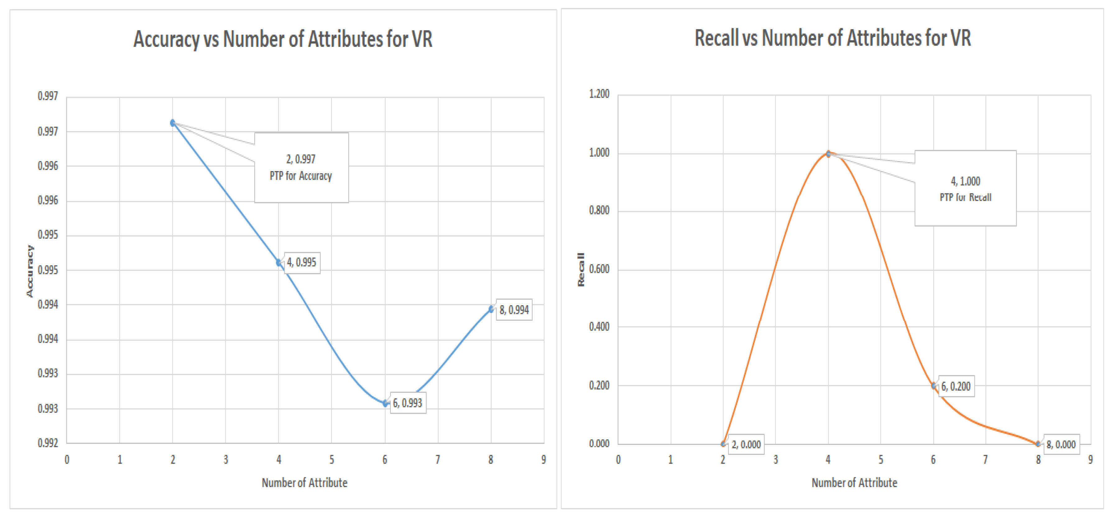
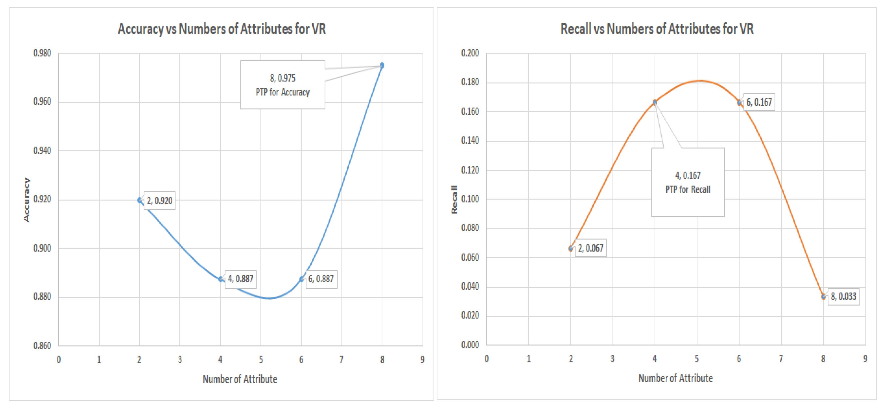
• Graphs: there are two main graphs in this section; their titles are “accuracy versus number of attributes for VR” and “recall versus number of attributes for VR”. Both graphs are plotted from the minority class. The graph “accuracy versus number of attributes for VR” will indicate the ${PeakThresholdPerformance}_{Accuracy}$ and is labeled in the graph as “PTP for accuracy”. The graph “recall versus number of attributes for VR” will indicate the ${PeakThresholdPerformance}_{minority}$ and is labeled in the graph as “PTP for accuracy”.

For this validation experiment, four subtable (two for Glass and two for Yeast) from the two main tables are used. The tables are “class 1 labeled as 1, others 0” and “class 3 re-labeled as class 1, others 0” from Table 7 for the Glass data. For the Yeast data, the subtables are “ERL as class 1, others as class 0” and “VAC as class 1, others as class 0” from Table 8.

7.3. Validation Experiments Using the Glass Dataset Results

For this validations experiment, two tables will be used, representing a section of much larger Table 7. The Glass dataset is highly imbalanced and multi-classed, each class represents a type of glass, such as tableware, car headlight, or window glass. are originally labeled as class 1, class 2, and so on up to class 7. However, class 4 is not available, so a total of six classes is present in the original datasets. The re-coding of multiple classes into “one-versus-all" was done and explained in earlier sections. However, to review, the re-coding involves labeling class 1 as class 1 and the other classes as class 0, then using it for the experiments after that round of experimentation. Then, class 2 is re-coded as class 1 and the others as class 0, and this setup is used for the experiments. Next, class 3 is re-coded as class 1 and others as class 0. This is continued until the experiment is complete. The example tabulation of the results is in Table 10 and all graphs are presented below. The minority table results were used for the graphs.

Table 10. Results of minority class for Glass data set for LR by variance ranking, Pearson correlation, and information gain feature selection for class 1 as 1 and others as class 0.

Minority Class
Algorithm	Number of Attributes	Accuracy	Precision	Recall	F-Measure	ROC	Total Captured
VR	2	0.617	0.400	0.343	0.369	0.644	24
	4	0.654	0.485	0.900	0.630	0.740	63
	6	0.659	0.488	0.871	0.626	0.777	61
	9	0.654	0.483	0.829	0.611	0.736	58
PC	2	0.617	0.400	0.343	0.369	0.644	24
	4	0.664	0.487	0.529	0.507	0.676	37
	6	0.650	0.474	0.643	0.545	0.714	45
	9	0.654	0.483	0.829	0.611	0.736	58
IG	2	0.678	0.509	0.414	0.457	0.643	29
	4	0.668	0.495	0.714	0.585	0.723	50
	6	0.668	0.495	0.771	0.603	0.749	54
	9	0.654	0.483	0.829	0.611	0.736	58

7.4. Logistic Regression Experiments for Glass Data Using One-Versus-All (Class 1 as 1 others as Class 0)

In this section, which is shown in Section 7.4 logistic regression experiments, where class 1 (70) is labeled as class 1 and other classes as class 0 (144). The VR outperformed the PC and IG with a value of 90% of recall of the minority, representing a total of 63 from 70 of the number of the minority data items. The graph of accuracy and recall for the minority is shown in Figure 8, and it shows the positions of accuracy and recall and the numbers of attributes that were to achieve the accuracy and recall.

Figure 8. Graph of LR accuracy and recall versus the numbers of attributes for Glass data minority class: class 1 as 1 and the others as class 0, ${PeakThresholdPerformance}_{Accuracy}$ and ${PeakThresholdPerformance}_{minority}$ in different positions.

7.5. Decision Tree (DT) Experiments for Glass Data Using One-Versus-All (Class 1 as 1 and the Others as Class 0)

Figure 9 shows the graph of decision tree results for the Glass data in the one-versus-all approach for class 1 re-coded as class I and the others as class 0. The minority class is our interest here; notice that the VR techniques captured more minority class groups than PC and IG did, with a recall of 56% at an accuracy of 69.6%, this result is a classic case of low accuracy but high recall. The graphs for the accuracy and recall versus numbers of attributes is in Figure 9 which shows that ${PeakThresholdPerformance}_{Accuracy}$ and ${PeakThresholdPerformance}_{minority}$ were the most significant attributes; they should be selected for the highest accuracy or highest recall of the minority.

Figure 9. Graph of decfision tree (DT) accuracy and recall versus numbers of attributes for the Glass data minority class: class 1 as 1 and the others as class 0, ${PeakThresholdPerformance}_{Accuracy}$ and ${PeakThresholdPerformance}_{minority}$ in different positions

7.6. Support Vector Machine (SVM) for Glass Data Using One-Versus-All (Class 1 as 1 the others as Class 0)

The SVM uses six attributes to attain the highest recall of 44.30% for the VR, while the highest levels for the PC and IG are recall rate of 37.1% and 38.6%, respectively. The SVM result was the only situation where the highest accuracy was attained with the lowest number of attributes (four), while the highest recall had six attributes.

During the Glass dataset validation experiments, the sub-table “class 1 as 1 and the others as class 0” was employed, the three algorithms that were used were the decision tree, logistic regression and support vector machine. In all the experiments VR captured more of the minority class data than PC and IG attribute selection did. These attributes were identified using the ${PeakThresholdPerformance}_{Accuracy}$ and ${PeakThresholdPerformance}_{minority}$ positions in the various graphs. The PC and IG are benchmark attribute selection techniques known in the data science community, but VR has been shown in many instances to produce equivalent or better results.

7.7. Logistic Regression Experiments for Glass Data Using One-Versus-All (Class 3 as Class 1 and the Others as Class 0)

The logistic regression algorithm worked best for this dataset and produced the only meaningful result. The other selected algorithm was unable to capture any minority class even if the accuracy was above 90%. for both the VR, PC, and IG. Although this may appear to be a failure, a closer analysis shows that what affects the state-of-the-art attribute selection like PC and IG also affects the invented VR. This supports the claims that VR belongs to the same league of attributes selection as the state-of-the-art, if not better.

7.8. Validation Experiments Using the Yeast Dataset Results

The components of the Yeast data make it an example of imbalanced datasets with the most classes in the data science community; see Figure 7 for Yeast data class contents proportion and Table 4 for the representation of the class re-coding as “one versus all”. There are 10 classes with varying degrees of imbalanced ratio (IR) between each class as class 1 and the rest classes (all) as class 0. The next sections present the experiments for DT, LR, and SVM for the attributes selected by VR, PC, and IG. Figure 10 shows the support vector machine accuracy and recall versus numbers of attributes for the Glass data minority class. While, Figure 11 illustrates the LR accuracy and recall versus numbers of attributes for Glass data minority class.

Figure 10. Graph of support vector machine (SVM) accuracy and recall versus numbers of attributes for the Glass data minority class: class 1 as 1 and the others as class 0, ${PeakThresholdPerformance}_{Accuracy}$ and ${PeakThresholdPerformance}_{minority}$ in different positions.

Figure 11. Graph of LR accuracy and recall versus numbers of attributes for Glass data minority class: class 3 as class 1 and the others as class 0 ${PeakThresholdPerformance}_{Accuracy}$ and ${PeakThresholdPerformance}_{minority}$ in different position.

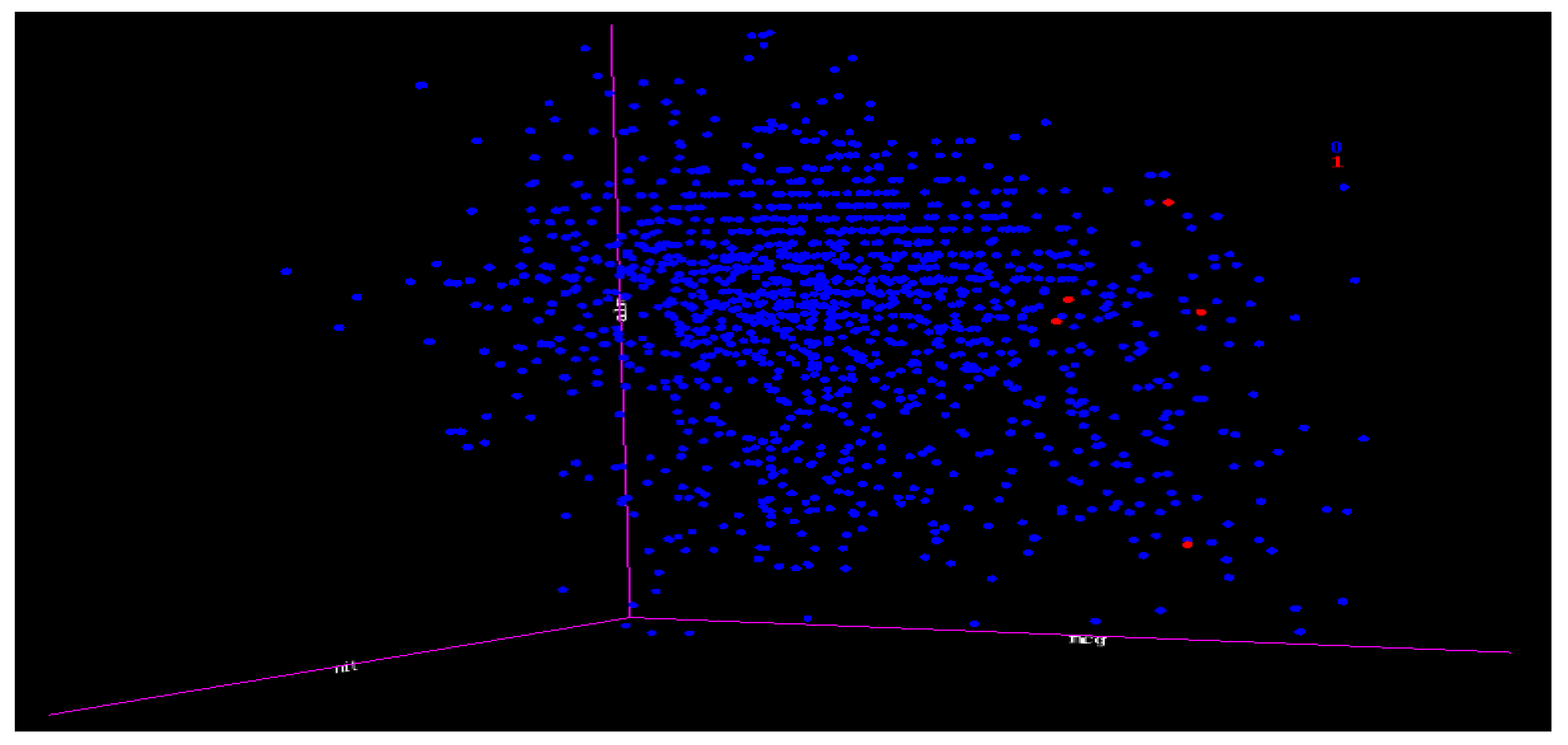
7.9. Decision Tree Experiments for Yeast Data Using One-Versus-All (Class ERL(5) as 1 and the Others as Class 0 (1479))

Table 11 relate to the DT experiment for class ERL(5) as class 1 and the others as class 0 (1479), the (IR) is 5:1479 or approximately 1:296. This means that for every one data item of class 1 (ERL), there are 296 data items of class 0 (others). This is an extreme case of imbalance, and Figure 12 shows how scanty class ERL(5) is as class 1 is in the midst of the others as class 0 (1479). Thus, even if the accuracy of the prediction is as high as above 99%, it may not even capture any minority data. The next session showed the graphs of minority data recalled at different numbers of attributes using the selected algorithms.

Table 11. Results of minority class for Yeast dataset for DT by variance ranking, Pearson correlation, and information gain feature selection for class ERL(5) as class 1, and the others (1479) as class 0.

Minority Class
Algorithm	Number of Attributes	(%) Accuracy	Precision	Recall	F-Measure	ROC	Total Captured
VR	2	0.996	0.000	0.000	0.000	0.480	0
	4	0.997	0.500	0.400	0.444	0.770	2
	6	0.996	0.333	0.200	0.250	0.697	1
	8	0.997	0.000	0.000	0.000	0.250	0
PC	2	0.997	0.500	0.200	0.286	0.890	1
	4	0.996	0.333	0.200	0.250	0.697	1
	6	0.996	0.333	0.200	0.250	0.697	1
	8	0.997	0.000	0.000	0.000	0.250	0
IG	2	0.996	0.000	0.000	0.000	0.480	0
	4	0.997	0.500	0.200	0.286	0.890	1
	6	0.996	0.333	0.200	0.250	0.697	1
	8	0.997	0.000	0.000	0.000	0.250	0

Figure 12. Extreme case of imbalance of class ERL(5) as 1 and the others as class 0 (1479).

In the decision tree (DT) experiment, the VR captured more of the minority data with four (4) number of attribute among those rankings with a recall value of 40%. The highest recall values of PC and IG is about 20%. The graph of ${PeakThresholdPerformance}_{Accuracy}$ and ${PeakThresholdPerformance}_{minority}$ is shown in Figure 13; this shows the most significant attributes. Thus, VR still performed better in capturing the minority member class.

Figure 13. Graph accuracy and recall versus numbers of attributes for Yeast class ERL(5) as 1 and the others as class 0 (1479) for a DT minority showing ${PeakThresholdPerformance}_{Accuracy}$ and ${PeakThresholdPerformance}_{minority}$ in the same positions

7.10. Logistic Regression (LR) Experiments for Yeast Data Using One-Versus-All (Class ERL(5) as 1 and the Others as Class 0 (1479))

The results are given in the graph in Figure 14. The logistic experiment performed better than the DT experiments carried out in earlier experiments with minority table results in Table 11.

Figure 14. Graph accuracy and recall versus numbers of attributes for Yeast class ERL(5) as 1 and the others as class 0 (1479) for LR minority showing ${PeakThresholdPerformance}_{Accuracy}$ and ${PeakThresholdPerformance}_{minority}$ in the same positions.

This is one of the best performances by variance ranking techniques, due to being able to capture the highest number of minority classes in an extremely imbalanced situation compared with the PC and IG. Once again, VR showed superiority over PC and IG, as demonstrated by the Yeast dataset with one-versus-all the sub-table of ERL(5) as class 1 and the others as class 0 (1479). This is an extreme case of imbalance because of the IR of 5:1478.

7.11. Decision tree (DT) and Support Vector Machine (SVM) Experiments for Yeast Data Using One-Versus-All (class VAC (30) as Class 1 and the Others as Class 0 (1454))

These two algorithm experiments were combined because their results were similar and they were unable to capture any minority in a case of extreme imbalance and extremely overlapping. Figure 15 is the 3D representation of the classes; notice the small numbers of the minority classes and how they are overlapped with the majority. This is regarded as an extreme case of imbalance.

Figure 15. Extreme case of imbalance class VAC(30) as 1 and the others as class 0 (1454).

The DT and SVM algorithms were unable to capture any minority when using any attribute selections including our VR. This shows that the effects of an extreme case of imbalance could also have effects on VR, PC, and IG. The importance of this is that whatever affects the benchmark attributes selections also affects our VR; hence, we make the case that the VR is equal to the established attribute selections in terms of performance, and in many instances, displayed a superior performance than the benchmark attribute selections.

7.12. Logistic Regression Experiments for Yeast Data Using One-Versus-All (Class VAC (30) as Class 1 and the Others as Class 0 (1454))

The results of the LR in Table 12 may initially appear odd because both variance ranking and Pearson correlation have the same results (same number of minority values captured). However, on close inspections of their comparison Table 8 for the Yeast dataset with “class VAC as class 1 and the others as class 0,” it can be observed that both attribute rankings are the same; as such; they should produce the same result. In the experiments, the variance ranking and Pearson correlation performed equally. The graph of ${PeakThresholdPerformance}_{Accuracy}$ and ${PeakThresholdPerformance}_{minority}$ is given in Figure 16.

Table 12. Results of minority class for Yeast dataset for LR by variance ranking, Pearson correlation, and information gain feature selection for class VAC(30) as class 1, and the others (1454) as class 0.

Minority Class
Algorithm	Number of Attributes	(%) Accuracy	Precision	Recall	F-Measure	ROC	Total Captured
VR	2	0.920	0.022	0.067	0.033	0.660	2
	4	0.887	0.034	0.167	0.056	0.660	5
	6	0.887	0.034	0.167	0.056	0.660	5
	8	0.975	0.111	0.033	0.051	0.660	1
PC	2	0.920	0.022	0.067	0.033	0.660	2
	4	0.887	0.034	0.167	0.056	0.660	5
	6	0.887	0.034	0.167	0.056	0.660	5
	8	0.975	0.111	0.033	0.051	0.660	1
IG	2	0.969	0.056	0.033	0.042	0.690	1
	4	0.913	0.037	0.133	0.058	0.690	4
	6	0.887	0.034	0.167	0.056	0.660	5
	8	0.975	0.111	0.033	0.051	0.660	1

Figure 16. Graph accuracy and recall versus numbers of attributes for Yeast class VAC(30) as 1 and the others as class 0 (1454) for the LR minority, showing ${PeakThresholdPerformance}_{Accuracy}$ and ${PeakThresholdPerformance}_{minority}$ in different position.

7.13. Conclusions

In this article, we demonstrated that the ranking of attributes done by VR could capture more minority class than those done by PC and IG. The experimentation starts with using all the attributes and eliminating their number by quarter until the best performance for highest accuracy and highest recall of the minority class is achieved, the point where this is achieved is called ${PeakThresholdPerformance}_{Accuracy}$ and ${PeakThresholdPerformance}_{minority}$ respectively. We also showed that both peak threshold performance may or may not happen at the same point, meaning at the same number of attributes. Remember that the problem of imbalance is that accuracy could be high while very few or sometimes no minority class group has been captured. By using various graphs of accuracy and recall versus numbers of attributes, we showed the position of ${PeakThresholdPerformance}_{Accuracy}$ and ${PeakThresholdPerformance}_{minority}$. In doing so, we provided a method of recognizing the most significant attributes that will capture more of the minority class data and also the position at which the predictive modeling will lose its dependability, these are some of the novelty of this research.

The experimentation and evidence provided in this section have shown that VR technique is usually superior and comparable to the benchmark attribute selections. In some of the experiments were the number of minority class data captured by VR, PC and IG are equal, the VR technique capture the same amount with less number attributes, hence using less resources, the implication of this is that VR could achieve the same level of performance with less number of attributes because it recognises the most relevant once better.

8. Comparison of Variance Ranking with Sampling (SMOTE and ADASYN)

SMOTE and ADASYN were explained in the literature review. They are only the two techniques that have used the IR just like our VR technique.

In these comparative experiments, we tried to replicate the SMOTE and ADASYN experiment as much as possible and compare their performance with that of VR. The idea is to ascertain the one that will produce the best performance in terms of accuracy and recall of the minority class groups. Three datasets, (Pima diabetes, Ionosphere, and Wisconsin cancer data) that was used in the initial experiment by [27] to the invent SMOTE in 2002 and also used by [28] to invent ADASYN in 2008 are still available in the public domain, and I have also used two of them extensively in this research.

The tables in Table 13 show the results for the experiments conducted for the comparisons, The relevant metrics are the ${PeakThresholdPerformance}_{Accuracy}$ represented by accuracy, the ${PeakThresholdPerformance}_{minority}$ represented by recall and the F-measure.

Table 13. Evaluation metric and performance comparison of VR, synthetic minority oversampling technique (SMOTE), and adaptive synthetic sampling (ADASYN).

Data Set	Techniques	Accuracy	Recall	F-measure	Data Set	Techniques	Accuracy	Recall	F-measure	Data Set	Techniques	Accuracy	Recall	F-measure
Pima	SMOTE-LR	0.691	0.535	0.507	Pima	SMOTE-DT	0.732	0.601	0.610	Pima	SMOTE-SVM	0.732	0.581	0.594
	ADASYN-LR	0.717	0.619	0.563		ADASYN-DT	0.733	0.600	0.612		ADASYN-SVM	0.733	0.600	0.612
	VR-LR	0.771	0.578	0.638		VR-DT	0.685	0.679	0.601		VR-SVM	0.742	0.612	0.616
Wiscosin	SMOTE-LR	0.927	0.864	0.892	Wiscosin	SMOTE-DT	0.924	0.899	0.889	Wiscosin	SMOTE-SVM	0.931	0.890	0.897
	ADASYN-LR	0.941	0.896	0.913		ADASYN-DT	0.923	0.900	0.888		ADASYN-SVM	0.937	0.901	0.908
	VR-LR	0.943	0.968	0.923		VR-DT	0.956	0.941	0.939		VR-SVM	0.967	0.954	0.952
Ionosphere	SMOTE-LR	0.849	0.735	0.785	Ionosphere	SMOTE-DT	0.880	0.762	0.821	Ionosphere	SMOTE-SVM	0.880	0.762	0.821
	ADASYN-LR	0.863	0.736	0.793		ADASYN-DT	0.872	0.740	0.812		ADASYN-SVM	0.895	0.825	0.843
	VR-LR	0.906	0.777	0.860		VR-DT	0.926	0.849	0.892		VR-SVM	0.926	0.838	0.893

Detailed graphs of the tables are also presented in Figure 17, Figure 18 and Figure 19. In the table, the results of SMOTE and ADASYN are compared with the results of VR. In the in logistic regression experiments for the Pima data, the ADASYN performed better in terms of recall, but in terms of accuracy, at 77.1%, the VR performed better; for the Wisconsin and Ionosphere data, the VR performed better in terms of both recall and accuracy. The Wisconsin data had values of 94.3% and 96.8% for accuracy and recall. For the Ionosphere, the VR also outperformed the SMOTE and ADASYN, with accuracy of 90.6% and recall of 77.7%. For clarity, the graph in Figure 17 shows the logistic regression experiments.

Figure 17. Graph evaluation metric and performance comparison for LR.

Figure 18. Graph evaluation metric and performance comparison for DT.

Figure 19. Graph evaluation metric and performance comparison for SVM.

The decision tree experiments in the second table of Table 13, the VR performed better than SMOTE and ADASYN in recalls. In the Pima data, the VR had a recall of 67.9%’ as against 60% and 60.1% for SMOTE and ADASYN; in Wisconsin, VR has a recall of 94.1%, while SMOTE and ADASYN had 90% and 89.9%, respectively. In the Ionosphere data, VR has a recall of 84.9%, while SMOTE and ADASYN had recalls of 74% and 76.2%.

Finally, in the support vector machine experiments, the VR also had a better recall for Pima data with 74.2% while SMOTE and ADASYN has Recalls of 58.1% and 60%. In the Wisconsin data, VR had a recall of 95.1% and SMOTE had 89% while ADASYN had 90.1%. The Ionosphere data were 83.8% for VR, while SMOTE and ADASYN had recall values of 76.2% and 82.5%, respectively.

9. Conclusions and Further Research

In this research, we proposed a novel techniques called variance ranking attribute selection for dealing with imbalanced class problems. We showed its superiority in the various experimentation and compared it with the two most popular attributes selections, PC and IG. We also compared VR with SMOTE and ADASYN, which are the main techniques for solving imbalanced data problems because both have utilized the IR. We have also demonstrated how the VR techniques use the one-versus-all to augments its performance.

One of the main advantages of VR is that it is not algorithm-dependent, and as such, could be applied to both supervised and unsupervised learning. In the predictive modeling lifecycle, at what stage should VR be carried out? The answer is simple: At the stage at which attribute selections are carried which is the data preprocessing stage. Using the VR as against other options may be the preferred alternative not only because it produces better results, but does so with the least number of attributes.

The variance ranking techniques is possible on only numeric data types, therefore future work will be extending the technique to categorical data by implementing a weighting strategy to enable a “summary statistics" on such data type. Finding a technique to calculate the descriptive statistics of categorical data is an active area of research for quite some time; one has to check the research data banks like google scholar to realize the enormity of the research interest. The new direction is, therefore, to utilize some of the research concepts to implements variance ranking on categorical data.

Classification algorithms are dichotomized, meaning the algorithm classifies a data point to belong to this class or that class, therefore is very possible to integrate variance ranking techniques into many machine learning algorithm for more augmented dichotomy which may improve the distinctions between the classes and improve the general performance of the algorithm, the future research implications are in the direction of integration of variance ranking and most machine learning algorithm.