Article

Feature Selection of Grey Wolf Optimizer Based on Quantum Computing and Uncertain Symmetry Rough Set

1
School of Automation, Harbin University of Science and Technology, Harbin 150080, China
2
Key Laboratory of Advanced Manufacturing and Intelligent Technology, Ministry of Education, Harbin 150080, China
3
Research Institute of Petroleum Exploration and Development Petro China Co Ltd., Beijing 100083, China
*
Author to whom correspondence should be addressed.
Symmetry 2019, 11(12), 1470; https://doi.org/10.3390/sym11121470
Submission received: 16 October 2019 / Revised: 24 November 2019 / Accepted: 28 November 2019 / Published: 2 December 2019

Abstract

:
Considering the crucial influence of feature selection on data classification accuracy, a grey wolf optimizer based on quantum computing and uncertain symmetry rough set (QCGWORS) was proposed. QCGWORS was to apply a parallel of three theories to feature selection, and each of them owned the unique advantages of optimizing feature selection algorithm. Quantum computing had a good balance ability when exploring feature sets between global and local searches. Grey wolf optimizer could effectively explore all possible feature subsets, and uncertain symmetry rough set theory could accurately evaluate the correlation of potential feature subsets. QCGWORS intelligent algorithm could minimize the number of features while maximizing classification performance. In the experimental stage, k nearest neighbors (KNN) classifier and random forest (RF) classifier guided the machine learning process of the proposed algorithm, and 13 datasets were compared for testing experiments. Experimental results showed that compared with other feature selection methods, QCGWORS improved the classification accuracy on 12 datasets, among which the best accuracy was increased by 20.91%. In attribute reduction, each dataset had a benefit of the reduction effect of the minimum feature number.

Graphical Abstract

1. Introduction

Feature selection (attribute reduction) is an effective data preprocessing step in the fields of pattern recognition and data mining. Davies and Russell proved that feature selection is a non-deterministic polynomial complete problem [1]. It aims to obtain the optimal feature subset from a problem domain. Feature subset selection maintains the same classification accuracy by deleting the irrelevant feature and the redundant features [2,3]. Designing and optimizing feature selection algorithm for different feature sets is the key to solve the problem of feature selection [4].
Many scholars have researched on feature selection methods. Two main methods for feature selection can be distinguished: the filter method and the wrapped approach [5]. The filter method is an early feature selection method [6], which uses the training set independent by the classifier to select feature subsets. Another approach to feature selection is the wrapped approach, which optimizes directly for a given learner. The final learning performance of the wrapped approach is better than that of the filtered approach. For improving the training accuracy of the deep learning tasks, these methods need to solve two problems: (i) How to evaluate the correlation of the feature subsets? (ii) How to explore different feature subsets?
In feature selection, a mathematical tool can deal with uncertain problems and reduce noisy features while keeping the attributes’ meaning. Rough set theory (RS), proposed by Pawlak, is effectively used as a tool to determine data dependencies and reduce the number of attributes from the dataset [7,8]. For feature subset evaluation, rough set theory is an objective to describe and deal with uncertain problems [9]. In order to apply rough set theory for dealing with attributes reduction of heterogeneity, some researchers proposed handling methods with rough set in the positive region. Mi et al. put forward a variable precision rough set reduction model based on the upper and lower approximation reduction matrices [10]. Qiu et al. studied the application of the f-rough principle as an evaluation rule [11]. Hu et al. established the k-nearest rough set model to evaluate the feature subset [12]. Furthermore, some researchers have optimized rough set methods based on changing discernable relationships to deal with feature selection for datasets with missing values. JERZYI et al. obtained more approximate informational decision rules by using valuable tolerance relations [13]. Qian et al. studied the discernible matrix of upper and lower approximation reduction and obtained the method of neighborhood rough set [14]. Yang et al. constructed a multi-granularity rough set selection model in incomplete information systems using tolerance relations [15]. Degangetal et al. presented a rough set attribute reduction method covering decision systems under the consistency and inconsistency [16]. Teng et al. used an entropy condition method to construct the attribute reduction model in the incomplete information system [17]. Grey wolf optimizer based on quantum computing and uncertain symmetry rough set (QCGWORS) was proposed to improve uncertain symmetry rough set theory based on a positive region to complete the evaluation of the feature subset of the incomplete information system.
The swarm intelligence optimization algorithm is a parallel, efficient, and global search method to simulate the biological behavior of group animals in a natural environment. These groups of individuals search for prey in a cooperative manner. Each member learns from the experience of other members of the group. As for the search strategy of feature subsets, the rough set theory and collaborative selection strategy of swarm intelligence have been proposed. For instance, a feature selection method using a rough set and genetic algorithm has improved classification accuracy [18]. Using a firefly algorithm, which is based on rough set theory, Long, N. C et al. worked out a spatial cooperative search strategy for feature subsets [19]. Wang, Inbarani, and Bae et al. studied the particle swarm optimization feature selection method for rough sets, effectively solving the pre-handling work in classification tasks [20,21,22]. Chen, Jensen, and Ke et al. used a rough set theory to optimize attribute reduction of ant colony optimization algorithm [23,24,25]. Chen et al. put forward a new fish swarm algorithm by using rough set theory for effective feature selection [26]. Based on the attribute reduction algorithm of the rough set, Luan et al. improved the strategy of the fish swarm algorithm [27]. Yamany et al. proposed a new search strategy by effectively integrating rough set theory with flower pollination optimization [28]. Yu et al. integrated accelerators into heuristic algorithms to optimize search strategies and improve the efficiency of feature extraction [29]. Grey wolf optimizer (GWO) is a popular swarm intelligence technique that has received widespread attention from scholars. The algorithm was inspired by grey wolves’ predation activity in nature [30]. The paper searched for feature subsets using the excellent search performance of the GWO algorithm.
For further improvement of the grey wolf optimization algorithm for feature selection, we used quantum computing to inspire it. Quantum computing refers to the manipulation of quantum systems in order to process information. The superposition principle of quantum mechanical states makes the state of quantum information units superimposed in multiple possibilities, which leads to greater potential for quantum information processing than efficiency for classical information processing [31].
QCGWORS took advantage of the global and local abilities of grey wolf optimizer and uncertain symmetry rough set theory to evaluate feature subsets. In addition, QCGWORS used quantum computing to inspire the grey wolf optimizer algorithm for feature selection.
In short, researchers have improved the evaluation scheme and search strategy of feature subsets. This paper designed a new cooperative swarm intelligence algorithm-QCGWORS algorithm, based on quantum computing and rough set theory, which is responsible for attribute reduction in the data classification task. Each feature subset represented the position of search individual in the space. This algorithm explored a search space composed of 2 m possible feature subsets for the m input feature conditions. The main goal of the algorithm was to apply parallel quantum computing to carry out feature subset optimization and evaluate the feature subset searched by a grey wolf optimizer by using rough set theory to test the feasibility of the algorithm.

2. Theoretical Basis of Combinatorial Optimization Feature Selection Algorithm

2.1. Uncertain Symmetry Rough Set

The rough set applies information systems and uncertain symmetry indiscernibility, and use approximate sets and features dependence to evaluate the selected feature subset and determines whether it is the optimal solution [32].
An information system is a collection of computer data that contains rows marked by objects; columns marked by features; elements marked with attribute values [33]. An information system may be extended by including decision features, and a specific example of an extended information system, which is extended by decision feature, is illustrated in Table 1. u, v, w are three conditional attributes, d is a decision attribute, and   z 1 , z 2 ,…, z 8 ( z i ) are the objects that belong to Z. If F = (Z,A∪{D}) is an information system, where Z is a non-empty finite set, U is a non-empty conditional feature finite set, and D is a set of finite decision features, then ∀u U produced the corresponding f u : Z → G u , making it produce G u corresponding to u.
Uncertain symmetry (US) is a metric of nonlinear correlation information that can be used to reveal the degree of relevance between two different nonlinear random variables. The information entropy H (L) of the random variable M is as follows:
H ( L ) = i P ( c i ) log 2 P ( c i ) ,
P( c i ) in Equation (1) represents the probability of the variable L = c i .
After observing random variable N, the information entropy of random variable M, namely conditional entropy H (L|N) is defined as:
H ( L | N ) = j P ( n j ) i P ( c i | n j ) log 2 P ( c i | n j )
where P ( n j ) represents the probability of the random variable N = n j , and P( c i | n j ) is called the posterior probability L under N.
After observing the random variable N and the information amount of the information entropy reduction of the random variable L, the information gain IG (L|N) is defined as:
I G ( L | N ) = H ( L ) H ( L | N ) .
Uncertain symmetry US (L,N) is a normalized information gain and is defined as:
U S ( L , N ) = I G ( L | N ) H ( L ) + H ( N ) .
For each feature subset of TU, the corresponding equivalence relation is as follows:
I N D ( T ) = { ( i , j ) Z × Z | u T , f u ( i ) = f v ( j ) } .
IND (T) represents the indistinguishable relation of T. The partition of Z generated by IND (T) is denoted as Z/T = { [ i ] t   ∈ U}. If (i, j) IND (T), i and j are indistinguishable attributes from T. [ i ] t is the equivalence class of the object, made up of all the elements.
If we set the lower approximation set of IZ as T _ I and upper approximation set as T ¯ I , the lower and upper approximations of I are defined by the following formula:
T _ I = { i U | [ i ] t I } ,
T ¯ I = { i U | [ i ] t I ϕ } .
We set T, M as two feature subsets of U, and let T, M be the equivalence relations over Z. The positive, negative, and boundary regions are shown as follows:
P O S T ( M ) = I Z / M T _ I ,
N E G T ( M ) = Z X Z / M T ¯ I ,
B N D T ( M ) = I Z / M T ¯ I X U / Q T _ I ,
POST(M), the positive region of partition Z/M relative to T, is a collection of all objects of Z, which can determine partition Z/M by T. M depends on T, and we can use TkM to represent k (0 ≤ k ≤ 1) in P:
k = γ T ( M ) = | P O S T ( M ) | | Z | .
Finding dependencies before features is an important task in data evaluation. γ T ( M ) is the dependency between condition feature T and decision feature M, and γ T ( M ) is also called the quality of approximation classification. If k = 1, M is dependent on T completely. If 0 < k < 1, M depends partly on T. However, if k = 0, M does not depend on T. The purpose of the attribute reduction is to remove redundant attributes from the rough set so that the reduction set can provide the similar classification quality as the original classification. A dataset may have many attribute reductions, and all reduction sets are defined as:
Re d ( W ) min = { O W | γ O ( D ) } = γ W ( D ) , V O , γ O ( D ) γ W ( D ) } ,
Re d ( W ) min = { O Re d | O Re d , | O | | O | } ,
where V, W are the conditional feature sets, and D is a decision feature set. Let O be a subset of W, then Red is called reductive reduction, where Red(W) is the reduced dataset of feature set W. γ O ( D )   is the dependence of condition feature O and decision feature D, and γ W ( D ) is the dependence of W and D. In particular, Red ( O ) min is the reduction with minimum cardinality, and it is called minimum reduction.

2.2. Quantum Computing

Quantum inspired computing is a new field of computer intelligence, which is a new computing method, based on quantum mechanics theory [34]. The superposition state of quantum can, therefore, lead to greatly increased computational speed in terms of complexity, as operations can be performed on multiple states simultaneously.
The basic unit of quantum computing is the quantum bit (qubit). The classical bit is the basic concept of classical computer science, which has two states of 0 or 1. A qubit has two possible states, | 0 and | 1 [35], where ‘ |   ’ is the Dirac notation, as it’s the standard notation in quantum computing. The superposition state of quantum computing is described as follows:
| ψ = α | 0 + β | 1 ,
where α and β are complex numbers that specify the probability amplitudes of the corresponding states.
An important operation in quantum computing is the quantum measurement, which converts a single qubit state into a probability classical bit. The probability of a 0 state is | α | 2 , or the probability of a state is | β | 2   .
An important operation in quantum computing is the measurement, which we represented by a ‘meter’ symbol. This operation converts a single qubit state | ψ = α | 0 + β | 1 into the probabilistic classical bit state, where |α|2 gives the probability of ‘0′state, |α|2 gives the probability of ‘1′state. The absolute square of the amplitude is the probability of measuring the qubit in the “0” or “1” state, and quantum computing always maintain the conservation of probability. This relationship equation is given as follows:
| α | 2 + | β | 2 = 1 .
Quantum measurement [36] is described by measurement operators M m , which act on the measured space and represent the possible measured results. Before measurement, the state of the quantum system is | ψ , and then the possibility of result m is as follows:
p ( m ) = ψ | M m + M m | ψ ,
The state of the system after the measurement is:
M m | ψ ψ | M m + M m | ψ ,
The equation satisfied by the measurement is as follows:
m M m + M m = 1 ,
The operation of the quantum gate can change the qubits’ state. The quantum gate can be described as a unitary operator ‘U’. It acts on the qubit basis states, satisfying U + U = UU + , where U + is the Hermitian adjoint of U. There are several quantum gates, such as the NOT gate, controlled NOT gate, rotation gate, Hadamard gate, etc. If there is a system of m quantum bits, the possible states of the quantum bits in the system can be up to 2 m state information. In the process of observing the state of the quantum, quantum computing would collapse the state of the qubit into a single certain state [36].

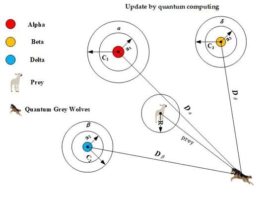
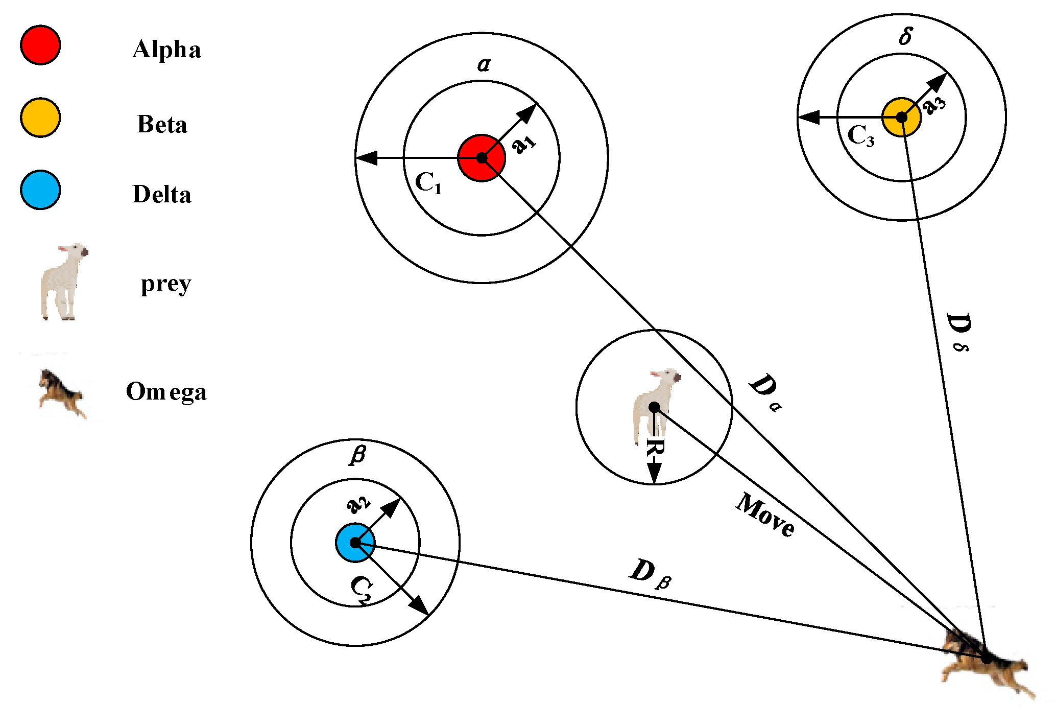
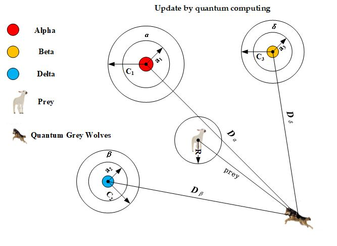
2.3. Grey Wolf Optimizer

GWO simulates the predation behavior of the grey wolf and applies the global search and local optimization exploration to the feature selection problem, improving the efficiency of searching the feature subset.
When designing the GWO, the first step is to build a social hierarchy model of grey wolves, calculate the fitness of each grey wolf individual of the population, and then mark the three grey wolves with the best fitness successively as alpha, beta, and delta, while the remaining grey wolves are labeled as omega [30]. That is, the grey wolf population ranks from the highest to the lowest: alpha, beta, delta, and omega. The optimization of GWO is mainly guided by the three best search wolves, alpha, beta, and delta.
All grey wolves have inherent characteristics of surrounding the prey during hunting. The enveloping behavior description established in the grey wolf optimizer is shown in Equations (19) and (20):
D = | C Y p ( t ) Y ( t ) | ,
Y ( t + 1 ) = Y p ( t ) A · D ,
D is the distance from the prey to the wolf, Y is the position vector of the wolf, Y p is the position vector of the prey at iteration t, and A and C are the random vectors. The calculation is
A = 2 a · r 1 a ,
C = 2 · r 2
the value of the vector a decreases linearly from 2 to 0 during the iteration, and r 1 , r 2 represent random vectors in [0, 1].
To simulate the search behavior of grey wolves (candidate solutions), the best three grey wolves (alpha, beta, delta) in the current population are retained during each iteration, and the positions of other search agents of wolves (omega) are updated based on their location information. The mathematical model of the behavior can be expressed as follows:
D Alpha = | C 1 · Y A l p h a Y | , D B e t a = | C 1 · Y B e t a Y | , D D e l t a = | C 1 · Y D e l t a Y | ,
Y 1 = Y A l p h a Y 1 Y A l p h a , Y 2 = Y B e t a A 2 D B e t a , Y 3 = Y D e l t a A 3 D D e l t a ,
Y ( t + 1 ) = Y 1 + Y 2 + Y 3 3 .
Y A l p h a , Y B e t a , Y D e l t a represent the position vectors of alpha, beta, and delta in the current population, respectively. Y represents the position vector of the grey wolf. Y A l p h a , Y B e t a , Y D e l t a represent the distance between the current candidate grey wolf and the optimal three wolves, respectively. A is a random value in the interval [−2a, 2a]. In the iteration process, when the random value of [−2a, 2a] is between [−1, 1], the next position of the grey wolf can be anywhere between its current position and the location of the prey. As shown in Figure 1, when | A | < 1, grey wolves are forced to attack the prey (local optimal solution).
As shown in Figure 2, when | A | > 1, the grey wolf is forced to separate from the current prey (the current local optimal solution) in the hope of finding a more suitable prey (the global optimal solution). Another component of the grey wolf optimizer (that is conducive to global optimization) can be seen from Equation (22) that the vector | C | contains random values in [0, 2]. The component provides a random weight for the prey to randomly enhance the prey of C   > 1 or not to enhance the prey of C   < 1, all of which are affected by the distance defined in Equation (22). It will help the grey wolf optimizer to show random behavior during the whole optimization process, which is conducive to global optimization and avoids local optimization.

3. Grey Wolf Optimizer Based on Quantum Computing and Rough Set

For the QCGWORS algorithm to solve the attributes reduction, the paper represented it in three main modules. The first module involved quantum in feature selection and initialization of grey wolf instances (in Section 3.3). In the second module (in Section 3.4), the solution of binary grey wolves was constructed from the way to update the search agent of a grey wolf optimizer (in Section 3.5).
The purpose of QCGWORS was to search for the potential optimal feature subset. First, it initialized some quantum grey wolf individuals in the optimized feature subset search space. Then, we got the group B G W 0 of n binary grey wolves from Q G W 0 by   the   algorithm   2 .   Binary grey wolf individuals explored the set space by searching for prey and hunting prey by algorithm 3. Grey wolf individuals searched this space to find the best three omega wolf solutions to update the positions of alpha, beta, and delta. Before reaching the maximum iterations of the algorithm, the fitness of individual grey wolves was calculated to determine whether to update search wolves’ positions. Then, the quantum superposition was used to represent the probability characteristics of selection, and the quantum gate was used to extract the characteristics of quantum measurement (value 1 means selected, value 0 means rejected). Finally, the concept of dependency proposed by the rough set theory was used to evaluate the feature selection, and it could determine whether a subset of conditional properties was an optimal solution. Algorithm 1 described the QCWCORS process.
Algorithm 1. QCGWORS process
Input: An extended Information System: F
Output: optimal feature subset R m i n
1.  Initialize n quantum grey wolf individuals Q G W 0 using (34);
2.  Get the group B G W 0 of n binary grey wolves from Q G W 0 by   the   Algorithm   2 .
3.  Search the minimal feature subset R x of each binary Wolf BGW x by the Algorithm 3;
4.   Evaluate   each   R x corresponding of binary wolf B G W x using (26);
5.   while (t < maximum iterations)
6.    for i=1:q (all q binary grey wolf individuals) do
7.  Evaluate the feature subset R x   using   ( 26 ) ;
8.  Update the best feature subset Red min   using   ( 13 ) ;
9.    end for
10.   end while
11.  return Red min end while
12. return Red min

3.1. Rough Set Evaluation Function

The uncertain symmetry is used to initially remove the irrelevant features, reduce the workload of feature selection, and strengthen the credibility of the feature subset evaluation. It can be seen from Equation (3) that if the variables L and N are not related, the information gain IG (L|N) =0, otherwise, IG (L|N) > 0; the larger the IG (L|N), between the variables L and N, the stronger the correlation. Therefore, IG(L|N) can be used quantitatively to assess the dependency between two variables. However, IG(L|N) can be affected by the variable unit and the variable value, so further homogenization is required.
We could find from Equation (4) that the uncertainty symmetry US(L, N) satisfies 0 ≤ US(L, N) ≤ 1; US(L, N) = 0 means that two random variables L and N are independent of each other, while (L, N) = 1 means that the two random variables L and N are completely related. According to the above theory, the relevant features are selected in the dataset, and the redundant feature can be removed to reduce the workload of feature selection, thereby improving the classification accuracy.
To evaluate the correlation between the conditional feature subset W and the decision feature D in the information system [20], the evaluation function is as follows
F i t n e s s = μ γ W ( D ) + τ | W O | | W |
γ O ( D ) is the dependence of conditional feature subset O with respect to decision feature D. | O | represents the subset O of the selected conditional features and satisfies O W; | W | represents the cardinality of the conditional features; μ   and   τ represent the influence of the dependency between the conditional feature subset O and the decision feature D. That is, it affects the reduction rate of O. μ     [ 0 , 1 ] ,   τ   =   1 μ . This equation shows that classification quality and attribute subset length have different meanings for attribute reduction task.
In order to calculate the degree of dependence between each conditional feature subset and decision feature, QCGWORS follows the following equations.
Compared to S 1 , a subset of the conditional feature, the three partitions of an unrecognized object are:
I N D ( S 1 ) = { { u 1 , u 3 , u 5 , u 7 } , { u 2 , u 6 } , { u 4 , u 8 } } ,
Compared to subsets of the conditional property S 2 , the three partitions of an indistinguishable object are:
I N D ( S 2 ) = { { u 1 , u 5 } , { u 2 , u 3 , u 6 , u 7 } , { u 4 , u 8 } } .
In summary, compared with the decision feature “class”, the two partitions of indistinguishable objects are:
D 1 = { u | c l a s s ( u ) = 0 = { u 1 , u 3 , u 5 , u 7 } } , D 2 = { u | c l a s s ( u ) = 0 = { u 2 , u 6 } } .
The algorithm finds out the positive region that can determine the IND and indiscernible relationship between the features S1, S2 and the decision feature D and, finally, calculates the dependency of conditional feature subset and decision feature. The dependencies between the decision feature set and S1 and S2 are as follows:
γ S 1 ( C l a s s ) = P O S S 1 ( C l a s s ) U ,
γ S 2 ( C l a s s ) = P O S S 2 ( C l a s s ) U .

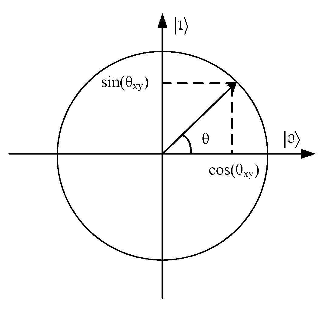
3.2. Quantum Representation of Grey Wolf Individual

This paper used the rotation angle [35] to represent qubit, the rotation angle is shown in Figure 1. Quantum grey wolf individual for feature selection: QGWx (the xth quantum grey wolf in a quantum group) corresponds to a vector Θ x . Θ x = ( θ x 1 , , θ x m ) of variables θ xy ,with θ xy ∈ [0, π 2 ] for (1 ≤ y ≤ m). Each quantum grey wolf solution QGW x is a string of qubits, calculated as follows:
Q G W x = [ cos ( θ x 1 ) | cos ( θ x m ) | sin ( θ x 1 ) | sin ( θ x m ) | ]

3.3. Quantum Computing in Feature Selection

In feature selection, there are two states for each feature subset: select or not select (1 or 0). This feature can be easily described by the two-dimensional quantum superposition state of 1 and 0 [31]. What needs to be done is to control the probability of updating the superposition when obtaining 1 or 0, so that the problem of feature selection can be solved in the field of quantum computing.
The quantum grey wolf population is represented by qubit sequences of length m, where m is the cardinal number of conditional attributes, and each qubit determines the selection probability of feature subset. The individual of the quantum grey wolf is represented by Q G W x , and the rotation angle is θ x , y . The relevant formula is as follows:
| Q G W x , y = cos ( θ x , y ) | 0 + sin ( θ x , y ) | 1 and ( cos 2 ( θ x , y ) ) + s i n 2 ( θ x , y ) ) = 1 )
Each quantum grey wolf Q G W 0 is initialized by:
Q G W 0 = ( cos ( π 4 ) | , cos ( π 4 ) | sin ( π 4 ) | , sin ( π 4 ) | )
where cos 2 ( π 4   ) is the probability that condition feature k will be selected, and sin 2 ( π 4   ) is the probability that k will be rejected.

3.4. Quantum Measurement in the Proposed Algorithm

In the operation of quantum measurement, the solutions of quantum grey wolf (QGWx) is used to generate a binary grey wolf (BGWx) solution by qubits’ projection. For a quantum bit, a random number r is generated from the interval [0, 1]. When r > sin2 ( θ x , y ), it sets to 1 to select the corresponding conditional feature; otherwise, the value is 0 and reject the corresponding conditional feature. Therefore, due to the superposition state of the qubits, a quantum superposition solution contains many binary solutions [37]. However, each qubit determines the probability of selecting or rejecting the corresponding feature. In the quantum measurement step, only certain binary solutions are extracted from quantum solutions, and the selection is guided by the probability of quantized coding.
By using the method of quantum measurement, a feasible feature selection solution of a binary grey wolf algorithm is constructed. At first, the algorithm does not select any feature. For each individual, according to R > sin2 ( θ x , y ), the feature is selected to refer to a condition, and the quantum measurement operation is repeated until all features are searched. The following algorithm 2 constructs the feasible solution B G W x   of feature selection by observing the Q G W x   of the quantum grey wolf. The process of algorithm 2 is as follows.
Algorithm 2. Quantum measurement in the proposed algorithm
Input: Q G W x : Quantum Grey individual, C= { c 1 ,   c 2 , , c x }: Conditional feature set
Output: B G W x : Binary Grey Wolf Individual, R x : Feature Subset
1.   R x ϕ
2.  for each qubit y of Q G W x do
3.  real value r is generated between [0, 1];
4.   if r > s i n 2 ( θ x , y ) then
5.   B G W x , y   ← 1;
6.  R ←   R x     c x , y ;
7.   else
8.   B G W x , y   ← 0;
9.   end if
10.  end for
11.  return B G W x

3.5. Update Position of Binary Grey Wolves

The process of using the binary grey wolf optimization algorithm begins with the initialization of the binary grey wolf individual in algorithm 2. During the iteration processes, alpha, beta, and delta estimate the possible positions of the feature subset (prey), and each potential feature subset scheme updates its distance from the prey. We can use A in [0, 2] to make the wolf diverge or converge from the prey. When A > 1, the candidate solution tends to stay away from the prey; when A <1, the candidate solution moves closer to the prey. The C vector in [0, 2] plays an important role in avoiding local optimal stagnation. C > 1 means that C emphasizes the role of avoiding local optimal. If C <1, the role of C will be randomly weakened. Finally, the grey wolf optimization algorithm terminates by satisfying the end criterion to obtain an alpha wolf. Algorithm 3.
Algorithm 3. Process of updating the binary wolves’ position
Input: I: Information System
Output: minimum condition feature subset R min
1.  Calculate the fitness of B G W 0
2.  Initialize search wolf for Alpha, Beta, and Delta.
3.  Initialize parameters a, A and C.
4.  while (t <Max iterations)
5.   for each Omega wolf
6.  calculate the fitness function (26) value of the B G W x  
7.    for each search wolf
8.     if there is a search wolf(Alpha, Beta, Delta) position that needs to be replaced
9.  Update parameters a, A and C.
10.  Update the current search wolf position
11.     end if
12.    end For
13.   end For
14.  end while
15.  return Alpha wolf, R m i n

4. Experiments

4.1. Experimental Setup

4.1.1. Classical Part Preparation

To verify the effect of the proposed QCGWORS intelligent collaboration algorithm on the feature selection, the experiments were based on 13 benchmark datasets collected from the machine learning repository of UCI (University of California Irvine) and OPENML platform (online at https://www.openml.org). In the experiment, we used a 64-bit Windows10 system with 16 G memory. MATLAB2014a was used as the simulation calculation tool of the algorithm, which is a commercial mathematics software produced by MathWorks, USA.
Thirteen datasets from the UCI database and OPENML platform are shown in Table 2. The features’ number and instances in the dataset were listed, respectively. There were four test experiments on collaborative grey wolf optimizer feature selection of quantum heuristic and rough set: QCGWORS algorithm improved the accuracy of classification tasks while the classification accuracy comparison experiment was conducted between the data processed by QCGWORS feature selection and the original data. Rough set evaluation and comparison experiments were conducted using QCGWORS rough set reduction method based on positive region and other rough set theoretical methods [38,39]. The QCGWORS was compared with the current popular rough set feature selection algorithm of swarm intelligent algorithms [26,40]. Swarm intelligence algorithm comparison experiment made comparison an effect among QCGWORS algorithm and ‘WOARSFS’ [40], ‘FSARSR’ [26] algorithms for feature selection. The experiment on the effect of the quantum part in feature selection made a comparison between the effect of the quantum part proposed algorithm QCGWORS and GWORS without the quantum part. In Table 2, KC1 and KC2 are two datasets from OPENML platform.
Attribute reduction rate and accuracy rate were used to evaluate the classification results of the best feature subset searched by the algorithm. In the decision tree algorithm of QCGWORS, the random forest (RF) algorithm and the k-nearest neighbor (KNN) algorithm were adopted, and the results of feature selection experiments were tested by means of cross-validation. The 10-fold cross-validation was adopted in the paper, and the dataset was divided into 10 parts, among which 9 parts were used as training data and 1 part as test data. The segmentation of data was repeated many times to ensure the reliability of the results and the accuracy of the data. Each experiment got the corresponding accuracy. The average value of 10 accuracy results served as the basis for the accuracy test of the algorithm.

4.1.2. Quantum Part Preparation

In order to prepare the basic environment of quantum computing, we used the MATLAB program package, Qubit4Matlabv3.0 [41]. As an additional package of MATLAB, it could help people build abstract quantum computing environment and implementation of quantum algorithms. It has the following related functions:
  • It can initialize the qubits and rearrange the qubits if needed;
  • It can easily construct the superposition state of qubits;
  • It can give abstraction to the quantum operator to easily format the quantum, such as NOT gate, quantum rotation gate, Hadamard gate, and other gate operation;
  • It can simplify quantum measurement operation to obtain the definite state of the qubit;
  • It can randomly generate correlation matrices, including unitary matrices.

4.2. Analysis of Experimental Data

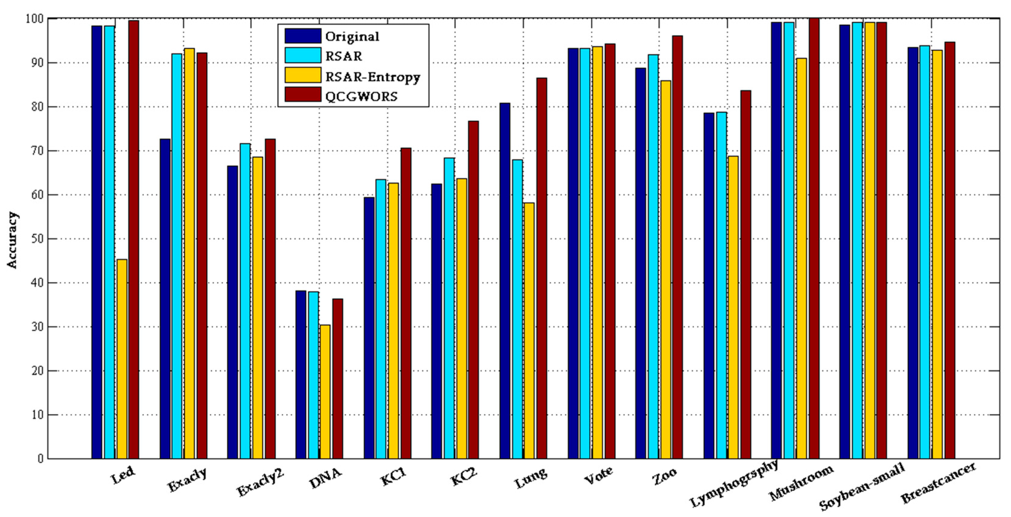
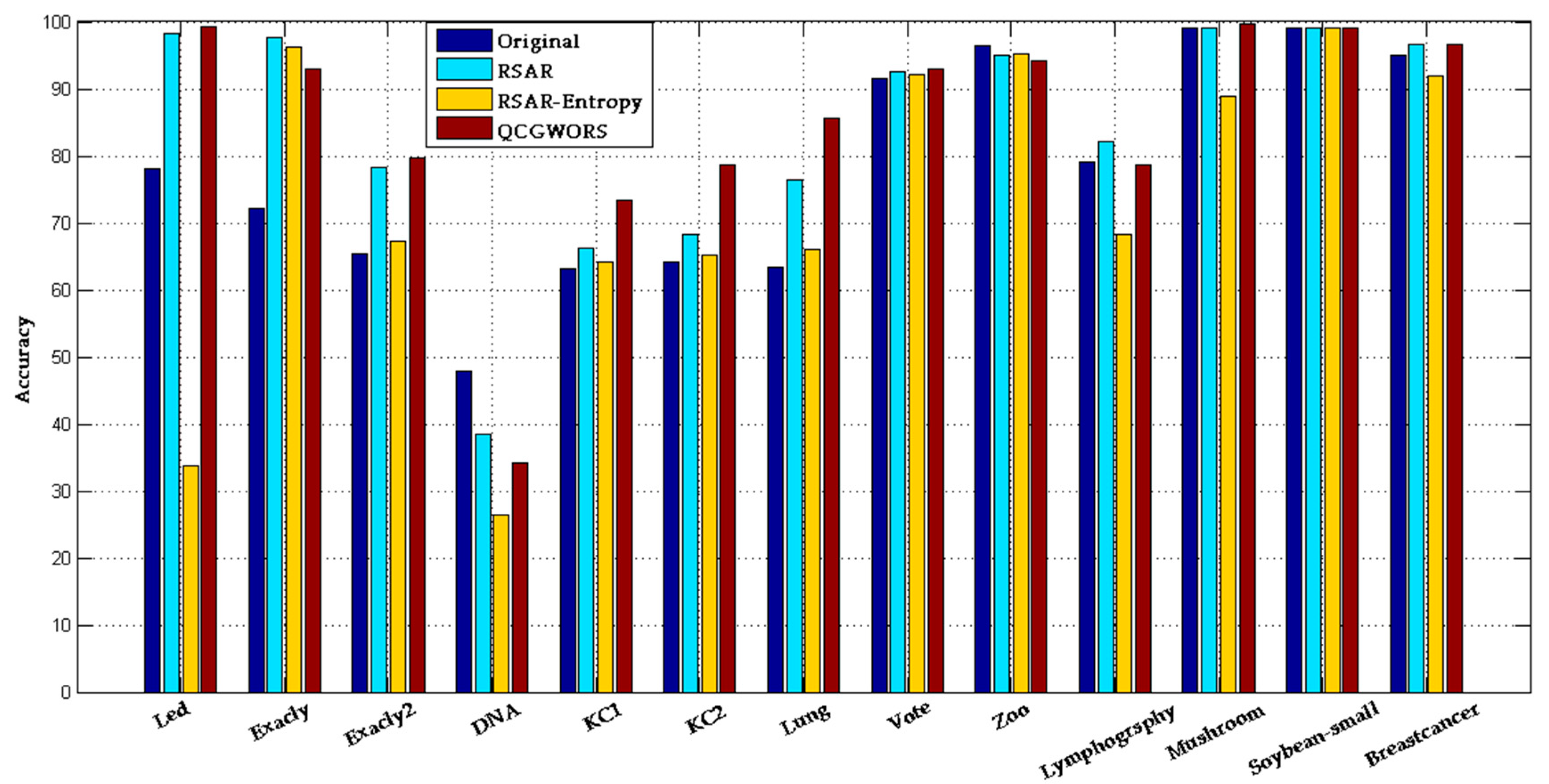
4.2.1. QCGWORS Improved Classification Accuracy Experiment

We made the experience between the proposed algorithm QCGWORS and original data without feature selection. Classification accuracy was calculated based on the percentage of the number of correct classifiers to the total number of original data. We used the random forest algorithm ‘RF’ and the k-nearest neighbor algorithm ‘KNN’ as classifier algorithms. In this part, the ten-fold cross-validation was used to ensure the accuracy of classification accuracy. The classification accuracy was added to the accuracy of each data, shown in Table 3. Data with bold fonts in Table 3 means that the classification accuracy of using the QCGWORS algorithm for feature selection was improved compared to the original data. The results in Table 3 show that the QCGWORS-attributed reduction rate and classification accuracy were greatly improved in almost all datasets. Especially in ‘Soybean-small’, ‘Lung’, ‘Breast cancer’, ‘DNA’, and ‘Mushroom’ data, the attribute reduction rate was more than 90%. In most cases, compared to the original data, the feature number of the optimal feature subset obtained using QCGWORS could improve the accuracy of the classification task.

4.2.2. Rough Set Evaluation and Comparison Experiment

The experiment verified the performance of rough set theory in attribute reduction. It used the rough set attribute reduction method of ’RSAR’ [38] and entropy reduction method of ‘RSAR-Entropy’ [39], and the QCGWORS algorithm of rough set theory attributed reduction based on positive region to conduct comparison experiments. The selection results of the best feature subset by the three algorithms are shown in Table 4. Where ‘RSAR’ represents using rough set attribute reduction method in experiment, ‘RSAR-Entropy’ reprsents rough set using entropy reduction method in experiment.
We could see from Table 4 that the selected quantity and the order of feature subsets were different. This was because RSAR used the dependency evaluation feature set, RSAR-entropy used the conditional entropy to evaluate the feature set, and QCGWORS used the uncertain symmetry rough set to evaluate the feature set.
Table 5 shows the attribute reduction effects and three feature selection algorithms using RSAR, RSAR-Entropy, and original data. Except for the RSAR algorithm ‘Lymphography’ dataset, the minimal feature subset for each dataset was obtained by the QCGWORS algorithm.
Based on the original data, RSAR, RSAR-Entropy, and QCGWORS experiments used the classifier of RF and KNN for data training, respectively. The comparison of training accuracy results using the RF classifier is shown in Figure 3, and the comparison of training accuracy results using the KNN classifier is shown in Figure 4. In the training results of the RF classifier, compared with the original data, the simplified data obtained by QCGWORS had 12 classification tasks that improved the accuracy. Comparing with the other two algorithms for attributes reduction, the QCGWORS obtained the highest accuracy in most dataset attribute reduction tasks, especially the best feature selection effect in the datasets of ‘Lymphography’, ‘Soybean-small’, and ‘Lung’. Furthermore, in the results of KNN classifier training, compared with the original data, the accuracy of the classification task processed by the QCGWORS algorithm was improved nine times.

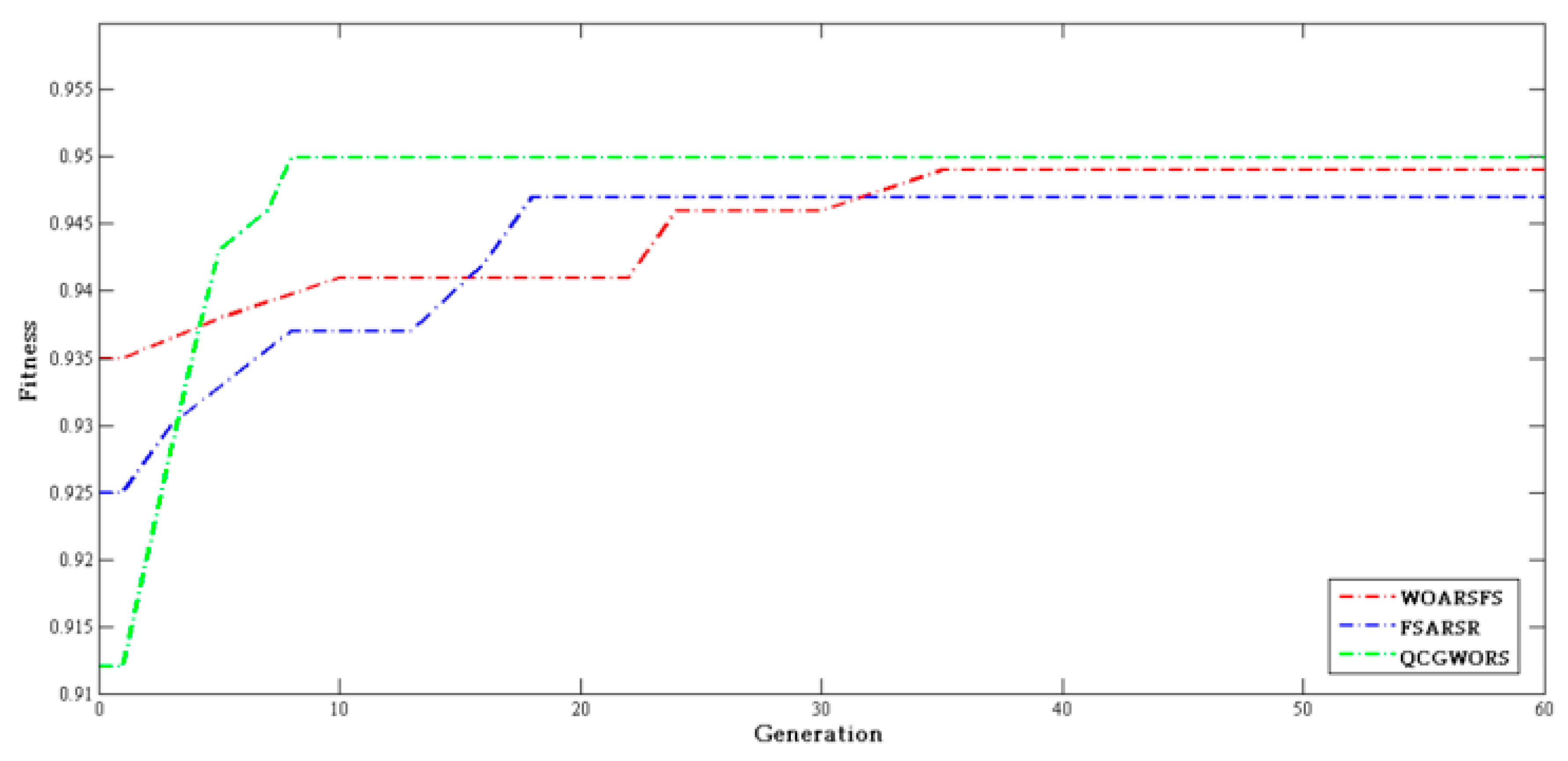
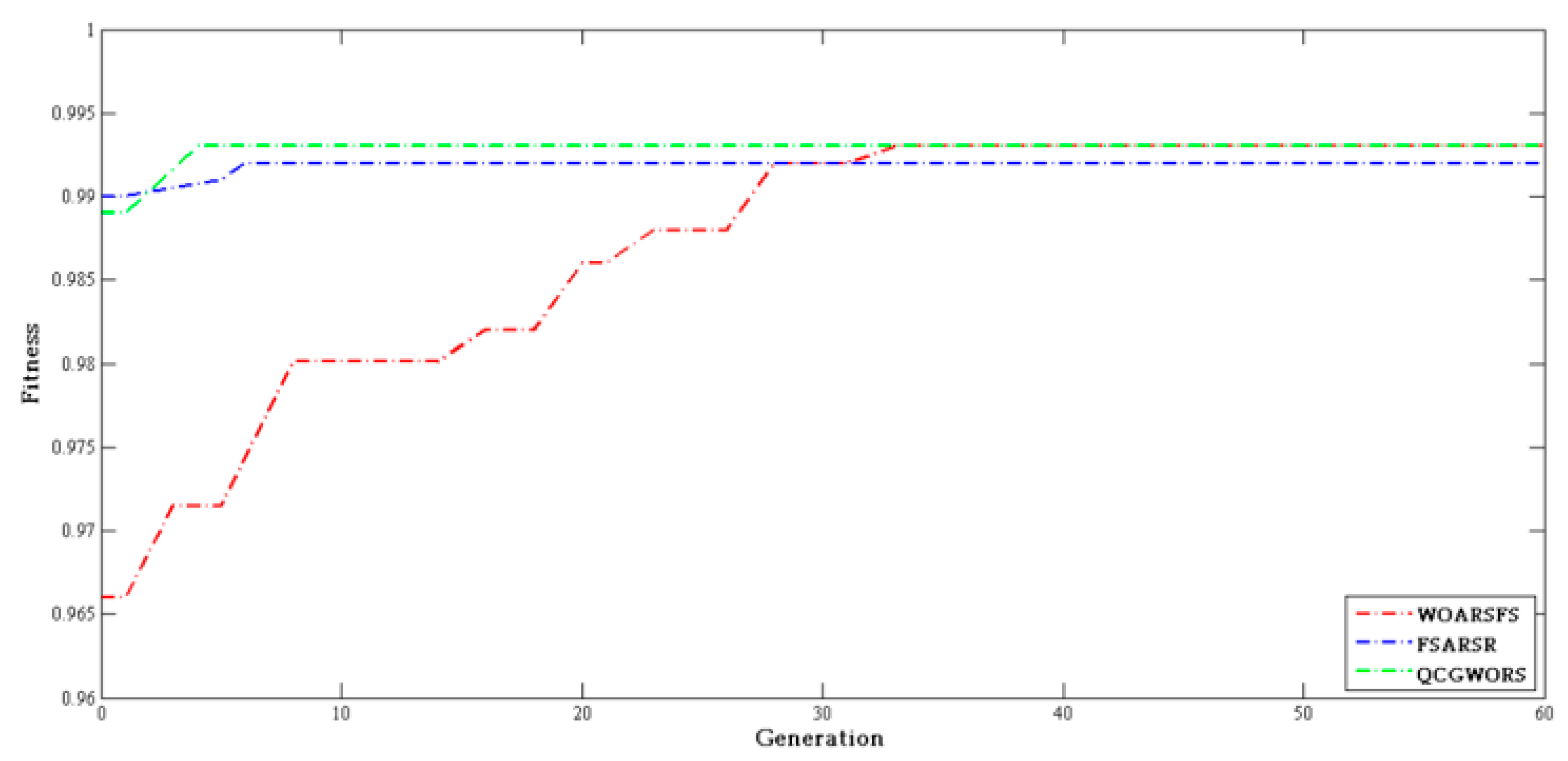
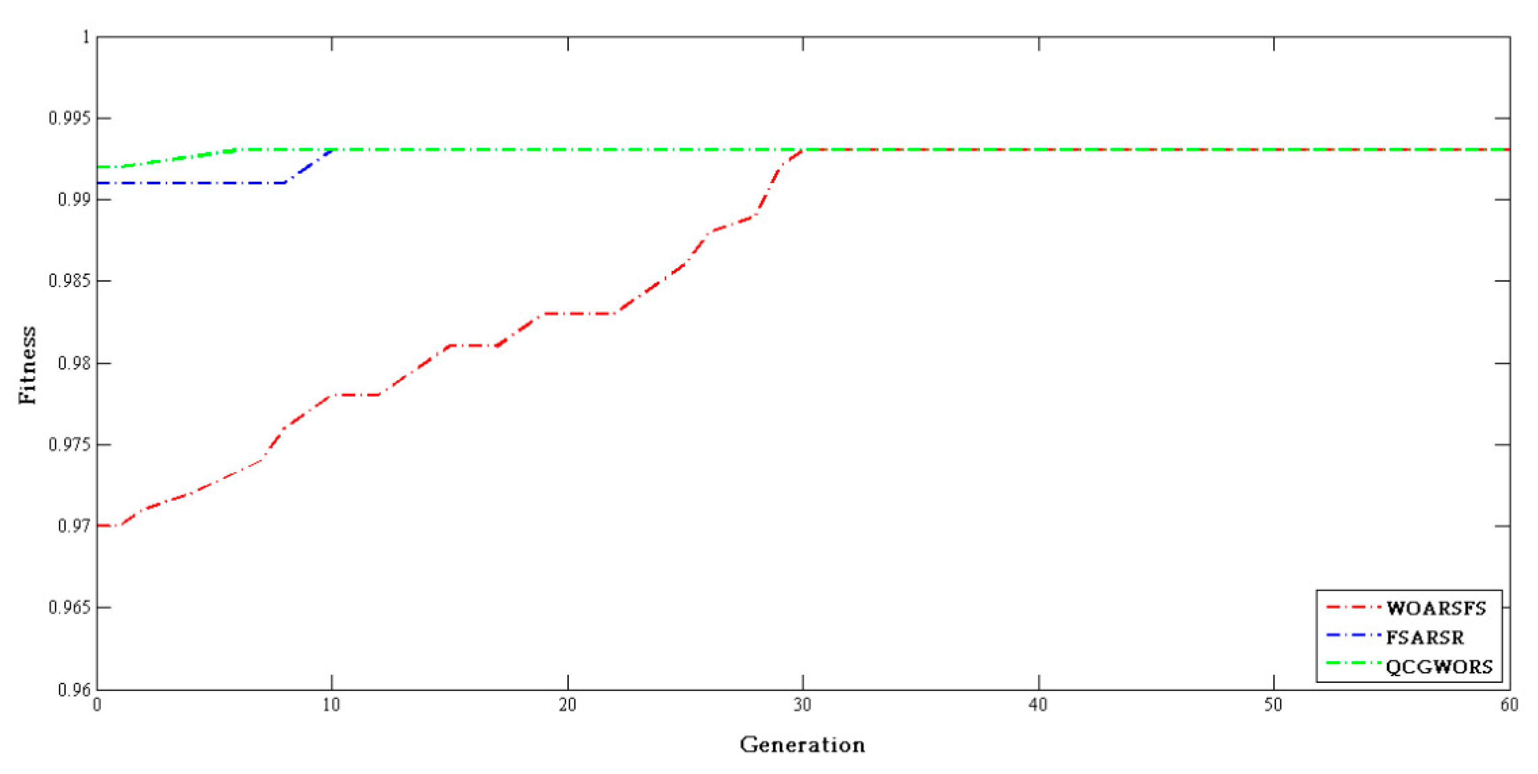
4.2.3. Swarm Intelligence Algorithm Comparison Experiment

In this part of the experiment, the performance of QCGWORS was compared with that of two other algorithms for the selection of swarm intelligence features of rough sets. In order to verify the effect of QCGWORS in feature selection more comprehensively, this experiment, based on the whale optimization rough set feature selection (WOARSFS) [40] and fish swarm algorithm rough set feature selection (FSARSR) [26], seeks for the comparison experiment between the WOARSFS, FSARSR, and QCGWORS, proving that the search strategy performance of QCGWORS was better than the current popular intelligent clustering algorithm. In terms of the influence of parameters on the above intelligent cluster algorithm in searching for the best dataset, we tried many times to select a better parameter scheme. There were relevant parameters that need to be supplemented in operation. For example, μ and   τ   were two parameters that mean the classification quality and the subset length; a and r were the values of the vectors a and r that affect the synergy coefficient when searching for prey; b was a constant for defining the shape of the logarithmic spiral. The size of quantum rotating angles θ was set as 0.025 π , based on multiple attempts. The parameters of the algorithm are shown in Table 6. The maximal number of iterations was 60 for the three algorithms.
The numbers of potential optimal feature subsets searched by the above three algorithms for attributes reduction are shown in Table 7. The fewer the number of features of the potential best feature subset found, the better the feature selection effect was. Compared with other swarm intelligence algorithms in all datasets, we could observe the following situation: In the case of ’KC1′, ‘KC2′, ’Lymphography’, and ‘Mushroom’ datasets, the QCGWORS provided better feature selection than FSARSR algorithm; in the case of ‘Lung’, ’Vote’, and ‘Soybean-small’ datasets, three intelligent swarm algorithms of rough sets searched for the same number of optimal feature subsets; in case of ‘DNA’ dataset, QCGWORS had better results of feature selection than ‘WOARSFS’ algorithm and ‘FSARSR’ algorithm. In the other datasets, the QCGWORS had better results of feature selection than the WOARSFS algorithm. Above all, compared with the above two rough set intelligent algorithms, the QCGWORS algorithm had stronger attribute reduction capabilities.
In order to ensure the fairness of three intelligent algorithm test experiments, we chose ‘Lung’ ‘Lympgography’, and ‘Soybean-small’ with the same number of feature subset in Table 7 for the experiment. WOARSFS, FSARSR, and QCGWORS are listed in Figure 5 for ‘Vote’, in Figure 6 for ‘Soybean-small’, in Figure 7 for ‘Lung’. In each figure, the fitness value represents the dependency of the optimal feature subset at each iteration, and it was calculated according to the Equation (26). Compared with the feature selection effect of WOARSFS, FSARSR, and QCGWORS, the least number of iterations were required to find the best feature subset. Three figures show the experimental results for all three datasets used in this comparison experiment. QCGWORS could find the best solution algorithm more quickly than WOARSFS and FSARSR. The experiment’s results clearly demonstrated that the QCGWORS algorithm for feature selection could explore the potential optimal subset of features more effectively in the search space.

4.2.4. Experiment on the Effect of Quantum Part in Feature Selection

In this experiment, we made a comparison of the effect between the proposed algorithm QCGWORS and GWORS without the quantum part. Classification accuracy was calculated based on the percentage of the number of correct classifiers to the total number of original data. We used the random forest algorithm ‘RF’ and the k-nearest neighbor algorithm ‘KNN’ as classifier algorithms. In this part, the ten-fold cross-validation was used to ensure the accuracy of classification accuracy. The classification accuracy was added to the accuracy of each data, shown in Table 3. Data with bold in Table 8 means the number of minimal features and classification accuracy obtained by using the QCGWORS algorithm improved the effect on feature selection compared to the GWORS. The results showed that QCGWORS obtained the minimal feature subset in the dataset ‘DNA’ and ‘Breast cancer’. The classification accuracy of QCGWORS was greatly improved in four cases. The use of the quantum part of the proposed algorithm, which was in feature selection, played an important role in optimization.
Based on the above experimental contents, QCGWORS was superior to other meta-heuristic feature selection algorithms in this paper. The advantages of the QCGWORS algorithm were reflected in higher classification accuracy, prominent feature reduction rate, and less iteration. The algorithm had passed four test experiments and finally achieved the ideal effect of finding the relevant feature subset. The good performance of the QCGWORS algorithm mainly benefitted from the efficient search space exploration strategy and the tailored correlation evaluation strategy for an incomplete information system. Experimental results showed that QCGWORS generally improved the classification accuracy and dimension reduction ability of datasets.

5. Conclusions

To solve the problem of low accuracy of feature selection in multidimensional data processing, we proposed a QCGWORS algorithm, which used quantum computing to improve the search strategy of grey wolf optimizer and uncertain symmetry rough set theory to evaluate the relevance of the generated feature subset. The classification accuracy was calculated by measuring the cross-validation method to evaluate the performance rate of QCGWORS. By testing and comparing QCGWORS on 13 datasets and other feature selection algorithms, experimental results showed that QCGWORS improved the classification accuracy and dimension reduction ability of datasets, and the accuracy of the classifier was increased by up to 20.91%, enabling each dataset to extract the minimum number of relevant features. QCGWORS played a crucial role in the burgeoning big data field. Moreover, it could be extended to a multi-objective version that uses several criteria to evaluate the characteristics of a subset after QCGWORS.

Author Contributions

Conceptualization, G.Z. and H.W.; Data curation, G.Z. and H.W.; Formal analysis, G.Z.; Funding acquisition, D.J. and Q.W.; Investigation, G.Z.; Methodology, H.W.; Project administration, G.Z.; Software, G.Z.; Supervision, H.W.; Validation, G.Z. and H.W.; Visualization, H.W.; Writing—original draft, G.Z.; Writing—review and editing, G.Z. and H.W.

Funding

This research was funded by the Key Project of Exploration and Production Branch of China National Petroleum Corporation ((Project No.: kt2017-17-01-1).

Conflicts of Interest

The authors declare no conflict of interest.

References

  1. References Davies, S.; Russell, S. NP-completeness of searches for smallest possible feature sets. In Proceedings of the AAAI Symposium on Intelligent Relevance, Berkeley, CA, USA, 4–6 February 1994; pp. 37–39. [Google Scholar]
  2. Gheyas, I.; Smith, L. Feature subset selection in large dimensionality domains. Pattern Recognit. 2010, 43, 5–13. [Google Scholar] [CrossRef]
  3. Vergara, J.; Estévez, P. A review of feature selection methods based on mutual information. Neural Comput. Appl. 2014, 24, 175–186. [Google Scholar]
  4. Mao, Y.; Zhou, X.B.; Xia, Z.; Yin, Z.; Sun, Y.X. Survey for study of feature selection algorithms. Pattern Recognit. Artif. Intell. 2007, 20, 211–218. [Google Scholar]
  5. Gan, J.; Hasan, B.; Tsui, C. A filter-dominating hybrid sequential forward floating search method for feature subset selection in high-dimensional space. Int. J. Mach. Learn. Cybern. 2014, 5, 413–423. [Google Scholar] [CrossRef]
  6. Kohavi, R.; John, G.H. Wrappers for Feature Subset Selection. Artif. Intell. 1997, 97, 273–324. [Google Scholar] [CrossRef]
  7. Pawlak, Z.; Skowron, A. Rough sets: Some extensions. Inf. Sci. 2007, 177, 28–40. [Google Scholar] [CrossRef]
  8. Pawlak, Z.; Skowron, A. Rudiments of rough sets. Inf. Sci. 2007, 177, 3–27. [Google Scholar] [CrossRef]
  9. Kryszkiewicz, M. Rough set approach to incomplete information systems. Inf. Sci. 1998, 112, 39–49. [Google Scholar] [CrossRef]
  10. Mi, J.S.; Wu, W.Z.; Zhang, W.X. Approaches to knowledge reduction based on variable precision rough set model. Inf. Sci. 2004, 159, 255–272. [Google Scholar] [CrossRef]
  11. Jinming, Q.; Kaiquati, S. F-rough law and the discovery of rough law. J. Syst. Eng. Electron. 2009, 20, 81–89. [Google Scholar]
  12. Hu, Q.; Yu, D.; Liu, J.; Wu, C. Neighborhood rough set based heterogeneous feature subset selection. Inf. Sci. 2008, 178, 3577–3594. [Google Scholar] [CrossRef]
  13. Stefanowski, J.; Tsoukias, A. Incomplete information tables and rough classification. Comput. Intell. 2001, 17, 545–566. [Google Scholar] [CrossRef]
  14. Qian, Y.; Liang, J.; Li, D.; Wang, F.; Ma, N. Approximation reduction in inconsistent incomplete decision tables. Knowl. Based Syst. 2010, 23, 427–433. [Google Scholar] [CrossRef]
  15. Yang, X.; Chen, Z.; Dou, H.; Zhang, M.; Yang, J. Neighborhood system based rough set: Models and attribute reductions. Int. J. Uncertain. Fuzziness Knowl. Based Syst. 2012, 20, 399–419. [Google Scholar] [CrossRef]
  16. Degang, C.; Changzhong, W.; Qinghua, H. A new approach to attribute reduction of consistent and inconsistent covering decision systems with covering rough sets. Inf. Sci. 2007, 177, 3500–3518. [Google Scholar] [CrossRef]
  17. Teng, S.H.; ZHOU, S.L.; SUN, J.X.; Li, Z.Y. Attribute reduction algorithm based on conditional entropy under incomplete information system. J. Natl. Univ. Def. Technol. 2010, 32, 90–94. [Google Scholar]
  18. Ren, Y.G.; Wang, Y.; Yan, D.Q. Rough Set Attribute Reduction Algorithm Based on GA. Comput. Eng. Sci. 2006, 47, 134–136. [Google Scholar]
  19. Long, N.C.; Meesad, P.; Unger, H. Attribute reduction based on rough sets and the discrete firefly algorithm. In Recent Advances in Information and Communication Technology; Springer: Berlin, Germany, 2014; pp. 13–22. [Google Scholar]
  20. Wang, X.; Yang, J.; Teng, X.; Xia, W.; Jensen, R. Feature selection based on rough sets and particle swarm optimization. Pattern Recognit. Lett. 2007, 28, 459–471. [Google Scholar] [CrossRef]
  21. Inbarani, H.H.; Azar, A.T.; Jothi, G. Supervised hybrid feature selection based on PSO and rough sets for medical diagnosis. Comput. Methods Programs Biomed. 2014, 113, 175–185. [Google Scholar] [CrossRef]
  22. Bae, C.; Yeh, W.C.; Chung, Y.Y.; Liu, S.L. Feature selection with intelligent dynamic swarm and rough set. Expert Syst. Appl. 2010, 37, 7026–7032. [Google Scholar] [CrossRef]
  23. Chen, Y.; Miao, D.; Wang, R. A rough set approach to feature selection based on ant colony optimization. Pattern Recognit. Lett. 2010, 31, 226–233. [Google Scholar] [CrossRef]
  24. Jensen, R.; Shen, Q. Fuzzy-rough data reduction with ant colony optimization. Fuzzy Sets Syst. 2005, 149, 5–20. [Google Scholar] [CrossRef]
  25. Ke, L.; Feng, Z.; Ren, Z. An efficient ant colony optimization approach to attribute reduction in rough set theory. Pattern Recognit. Lett. 2008, 29, 1351–1357. [Google Scholar] [CrossRef]
  26. Chen, Y.; Zhu, Q.; Xu, H. Finding rough set reducts with fish swarm algorithm. Knowl. Based Syst. 2015, 81, 22–29. [Google Scholar] [CrossRef]
  27. Luan, X.Y.; Li, Z.P.; Liu, T.Z. A novel attribute reduction algorithm based on rough set and improved artificial fish swarm algorithm. Neurocomputing 2016, 174, 522–529. [Google Scholar] [CrossRef]
  28. Yamany, W.; Emary, E.; Hassanien, A.E.; Schaefer, G.; Zhu, S.Y. An innovative approach for attribute reduction using rough sets and flower pollination optimisation. Procedia Comput. Sci. 2016, 96, 403–409. [Google Scholar] [CrossRef]
  29. Chen, Y.; Zeng, Z.; Lu, J. Neighborhood rough set reduction with fish swarm algorithm. Soft Comput. 2017, 21, 6907–6918. [Google Scholar] [CrossRef]
  30. Mirjalili, S.; Mirjalili, S.M.; Lewis, A. Grey wolf optimizer. Adv. Eng. Softw. 2014, 69, 46–61. [Google Scholar] [CrossRef]
  31. Schuld, M.; Sinayskiy, I.; Petruccione, F. An introduction to quantum machine learning. Contemp. Phys. 2015, 56, 172–185. [Google Scholar] [CrossRef]
  32. Yu, L.; Liu, H. Efficient feature selection via analysis of relevance and redundancy. J. Mach. Learn. Res. 2004, 5, 1205–1224. [Google Scholar]
  33. Swiniarski, R.W.; Skowron, A. Rough set methods in feature selection and recognition. Pattern Recognit. Lett. 2003, 24, 833–849. [Google Scholar] [CrossRef]
  34. Benioff, P. The computer as a physical system: A microscopic quantum mechanical Hamiltonian model of computers as represented by Turing machines. J. Stat. Phys. 1980, 22, 563–591. [Google Scholar] [CrossRef]
  35. Nielsen, M.A.; Chuang, I. Quantum computation and quantum information. Am. J. Phys. 2002, 70, 558–694. [Google Scholar] [CrossRef]
  36. Manju, A.; Nigam, M.J. Applications of quantum inspired computational intelligence: A survey. Artif. Intell. Rev. 2014, 42, 79–156. [Google Scholar] [CrossRef]
  37. Zouache, D.; Nouioua, F.; Moussaoui, A. Quantum-inspired firefly algorithm with particle swarm optimization for discrete optimization problems. Soft Comput. 2016, 20, 2781–2799. [Google Scholar] [CrossRef]
  38. Jensen, R.; Shen, Q. Finding Rough Set Reducts with Ant Colony Optimization. J. Fussy Sets Sys. 2003, 49, 15–22. [Google Scholar]
  39. Wang, G.; Yu, H.; Yang, D.C. Decision table reduction based on conditional information entropy. Chin. J. Comput. Chin. Ed. 2002, 25, 759–766. [Google Scholar]
  40. Tharwat, A.; Gabel, T.; Hassanien, A.E. Classification of toxicity effects of biotransformed hepatic drugs using whale optimized support vector machines. J. Biomed. Inform. 2017, 68, 132–149. [Google Scholar] [CrossRef]
  41. Tóth, G. QUBIT4MATLAB V3. 0: A program package for quantum information science and quantum optics for MATLAB. Comput. Phys. Commun. 2008, 179, 430–437. [Google Scholar]
Figure 1. Qubit representation by the unity circle.
Symmetry 11 01470 g001
Figure 2. Operation mechanism of grey wolf optimizer.
Symmetry 11 01470 g002
Figure 3. Comparative histograms using the random forest (RF) method for classification.
Symmetry 11 01470 g003
Figure 4. Comparative histograms using the k nearest neighbors (KNN) method for classification.
Symmetry 11 01470 g004
Figure 5. Histogram of experimental comparison of ‘Vote’ data.
Symmetry 11 01470 g005
Figure 6. Histogram of experimental comparison of ‘Soybean-small’ data.
Symmetry 11 01470 g006
Figure 7. Histogram of experimental comparison ‘Lung’ of data.
Symmetry 11 01470 g007
Table 1. Extended information system.
z i Z uvwd
z 1 0110
z 2 1110
z 3 1001
z 4 0000
z 5 1010
z 6 0011
z 7 1100
z 8 0000
Table 2. Dataset parameters.
No.DatasetFeaturesSamples
1Led242000
2Exactly131000
3Exactly2131000
4DNA57318
5KC1222109
6KC221522
7Lung5632
8Vote16300
9Zoo16101
10Lymphography18148
11Mushroom228124
12Soybean-small3547
13Breast cancer9699
Table 3. Analysis data of classification accuracy effect.
DatasetORIGINALQCGWORS
FeaturesRFKNNFeaturesRFKNN
Led2498.20 ± 0.5077.99 ± 0.8599.57 ± 0.3299.31 ± 0.25
Exactly1372.53 ± 2.5072.14 ± 0.7692.23 ± 0.9093.05 ± 0.30
Exactly21366.51 ± 1.5065.38 ± 0.51072.56 ± 0.0579.63 ± 0.7
DNA5737.96 ± 21377.80 ± 0.9536.25 ± 0.2334.09 ± 0.10
KC12259.23 ± 2.5161.14 ± 2.92870.42 ± 0.1673.42 ± 1.37
KC22162.25 ± 2.1764.25 ± 1.92576.61 ± 0.2378.61 ± 0.81
Lung5680.78 ± 0.2763.28 ± 2.64486.35 ± 0.1685.53 ± 0.74
Vote1693.08 ± 0.6391.62 ± 0.65894.12 ± 0.6992.88 ± 0.42
Zoo1688.74 ± 1.0396.34 ± 0.43596.06 ± 0.1494.21 ± 0.40
Lymphography1878.38 ± 2.2079.07 ± 1.52783.49 ± 2.0178.75 ± 1.22
Mushroom2299.00 ± 1.0799.00 ± 0.10499.03 ± 0.1099.71 ± 0.10
Soybean-small3598.47 ± 2.5399.00 ± 0.10299.00 ± 0.1099.00 ± 0.10
Breast cancer993.44 ± 6.5694.94 ± 0.51494.65 ± 0.7396.59 ± 0.34
Average2579.1277.80685.1785.59
Table 4. Selection of feature subset.
Dataset‘RSAR’‘RSAR-Entropy’‘QCGWORS’
Led6,1,2,4,3,56,11,24,19,22,8,18,21,9,16,7,11,2,3,4,5
Exactly1,2,3,4,5,11,7,93,5,7,1,4,8,9,111,3,5,7,9,11
Exactly21,2,3,4,10,9,6,8,7,52,3,8,6,13,12,5,10,11,4,71,2,3,4,5,6,7,8,9,10
DNA1,16,45,24,57,2,318,42,14,49,9,255,19,22,26,33
KC14,2,5,8,9,7,10,11,1,61,5,2,7,3,11,4,21,15,182,4,5,6,7,8,11,18
KC22,4,5,8,7,18,11,62,5,6,8,7,4,1,18,52,4,5,7,8
Lung1,42,7,43,9,4,36,13,153,9,24,42
Vote1,4,12,16,11,3,13,2,99,16,8,14,5,10,13,2,15,4,61,2,3,4,9,11,13,16
Zoo4,13,12,6,86,13,1,8,7,5,15,14,12,33,4,6,8,13
Lymphography2,18,14,13,16,151,18,14,5,12,11,16,28,6,2,13,14,18,15
Mushroom5,20,8,12,314,1,9,3,65,12,20,22
Soybean-small4,2223,2223,22
Breast cancer1,7,2,61,3,4,91,6,5,8
Table 5. Raw data and simplified data using three feature selection algorithms.
DatasetOriginalRSARRSAR-EntropyQCGWORS
Led246115
Exactly13886
Exactly213101110
DNA57765
KC12211108
KC221795
Lung56454
Vote169118
Zoo165105
Lymphography18687
Mushroom22554
Soybean-small35222
Breast cancer246115
Table 6. Algorithm parameter settings.
AlgorithmParameters
WOARSFSPopulation size = 20, τ   = 0.9,   μ = 0.1, a ( 0 , 2 ) ,   r ( 0 , 1 ) ,   b = 1
FSARSRPopulation size = 20, τ   = 0.9,   μ = 0.1
QCGWORSPopulation size = 20, τ   = 0.9,   μ   = 0.1,   θ   size   is   0.025 π , a ( 0 , 2 ) ,   r ( 0 , 1 )
Table 7. The number of features of the potential best feature subsets found by different feature selection algorithms.
DatasetFeaturesWOARSFFSARSRQCGWORS
Led24655
Exactly13766
Exactly213111010
DNA57675
KC122898
KC221565
Lung56444
Vote16999
Zoo16655
Lymphography18787
Mushroom22454
Soybean-small35222
Breast cancer24655
Table 8. Comparison of QCGWORS with GWORS.
DatasetFeatureGWORSQGWORS
RFKNNFeatureRFKNNFeature
Lung5684.03 ± 0.2285.21 ± 0.81486.35 ± 0.1685.53 ± 0.744
DNA5735.13 ± 0.2033.78 ± 0.10736.25 ± 0.2334.09± 0.105
Vote1691.41 ± 0.2990.64 ± 0.45893.12 ± 0.6992.88 ± 0.428
Breast cancer2492.21 ± 0.2893.91 ± 0.57594.65 ± 0.7396.59 ± 0.344

