An Evidential Prospect Theory Framework in Hesitant Fuzzy Multiple-Criteria Decision-Making

Abstract

In numerous real decision-making problems, decision-makers (DMs) encounter situations involving hesitant and probabilistic information simultaneously, and DMs show behavior characteristics of nonrational preferences when they encounter decision-making situations with uncertain information. To address such multiple-criteria decision-making (MCDM) issues with hesitant and probabilistic information and nonrational preferences, a novel method, called the evidential prospect theory framework, is developed herein based on evidence theory and prospect theory, where the associated coefficients in prospect theory are given on the basis of symmetry principles (i.e., the associated coefficients are common knowledge to DMs). Within the proposed method, belief structures derived from evidence theory apply to the experts’ uncertainty about the subjective assessment of criteria for different alternatives. Then, by combining belief structures, the weighted average method is applied to estimate the final aggregated weighting factors of different alternatives. Furthermore, considering the nonrational preferences of DMs, the expected prospect values of different alternatives are derived from the final aggregated weighting factors and prospect theory, which is applied to the ranking order of all alternatives. Finally, a case involving a parabolic trough concentrating solar power plant (PTCSPP) is shown to illustrate the application of the novel method proposed in this paper. The evidential prospect theory framework proposed in this paper is effective and practicable, and can be applied to (green) supplier evaluation.

1. Introduction

In multiple-criteria decision-making (MCDM) problems, fuzzy set theory, proposed by Zadeh, is an effective alternative to characterize uncertainty and complexity [1]. Fuzzy set theory can systematically process linguistic information from decision-makers (DMs) or experts in decision-making problems [2,3]. In traditional MCDM, there exists a basic assumption that DMs are rational [4,5,6,7]. Nevertheless, DMs are usually not rational decision-makers, and real decision-making behavior often deviates from the prediction of expected utility. That is, DMs’ nonrational preferences have a critical impact on the associated decision-making results. To characterize DMs’ nonrational preferences, some non-expected utility functions have been proposed, such as prospect theory [7], rank-dependent utility [8], and loss aversion utility [9]. The most striking of the non-expected utility functions is prospect theory. Prospect theory is the most influential theory of decision-making with uncertain information. Different from expected utility theory, prospect theory evaluates the outcomes with respect to some reference outcome, where gains or losses are called prospects. The value function in prospect theory characterizes the phenomenon that losses loom larger than gains. The probability weighting function describes the phenomenon that DMs overweight (or underweight) small (moderate to large) probabilities. The empirical works on psychological behavior justify prospect theory [10]. That is, decisions made based on prospect theory are in line with real decision-making [11,12,13,14].

In addition, in MCDM problems, fuzzy set theory provides an effective mathematical method to process the uncertainty of DMs’ judgement. A DM’s mind can be highly modeled by the linguistic variables that are characterized by fuzzy numbers. For instance, “the car is good”, “the stability is high”, and so on. However, it fails to adequately describe a more complex situation involving hesitant and probabilistic information simultaneously. For example, the mobile phone is good at a probability of 0.7, and the mobile phone is “medium good” at a probability of 0.3, etc. For such situations, Dempster and Shafer proposed evidence theory [15,16]. As a reasoning method for uncertain information, a belief structure derived from evidence theory can adequately represent the uncertainty involving DMs’ judgement [17,18,19], which apples to numerous fields, including pattern recognition [20,21], risk assessment [22,23], identification of influential nodes [24,25], etc. [26,27,28]. By making use of belief structures, the various types of uncertainty in the decision-making process can be described adequately. This paper adopts belief structures to describe the decision-making situations involving hesitant and probabilistic information simultaneously.

By reviewing the above works on MCDM problems, it was found that there are some gaps in the extant literature. (1) Although the psychological preferences of DMs are considered in the extant MCDM works based on prospect theory, these works do not involve the various types of uncertainty, such as hesitant and probabilistic information. That is, the method based on prospect theory cannot deal with MCDM problems involving hesitant and probabilistic information simultaneously. (2) Evidence theory addresses the problems of the various types of uncertainty in the existing MCDM works, but the literature fails to consider the psychological preferences of DMs, except Nusrat and Yamada [29]. However, Nusrat and Yamada only showed a descriptive decision-making model and ignored the various types of uncertainty in the decision-making process.

Consequently, a novel method is proposed in this paper. It takes into account the following two situations: (1) DMs show nonrational preferences that are taken into account based on prospect theory; (2) the experts’ subjective judgment of criteria involves hesitant and probabilistic information simultaneously. In this paper, we consider an MCDM problem with hesitant and probabilistic information, where DMs present behaviors of nonrational preferences. A novel method, called the evidential prospect theory framework, is developed based on evidence theory and prospect theory. Within the proposed framework, belief structures derived from evidence theory are applied to characterize the experts’ uncertainty about the subjective assessment of criteria for different alternatives, which involves hesitant and probabilistic information simultaneously. Prospect theory models DMs’ nonrational preferences. Then, by combining belief structures, the weighted average method is applied to estimate the final aggregated weighting factors of different alternatives. Furthermore, the expected prospect values of different alternatives are derived from the final aggregated weighting factors and prospect theory, which is applied to the ranking order of all alternatives.

Compared to the existing models that address MCDM problems, the evidential prospect theory framework has two advantages: First, the proposed framework characterizes decision-making situations involving hesitant and probabilistic information simultaneously. Second, the proposed framework considers DMs’ nonrational preferences. Since the extant works still have not referred to hesitant and probabilistic information and nonrational preferences simultaneously, the proposed framework fills the research gap involving hesitant and probabilistic information and nonrational preferences simultaneously in MCDM problems. In addition, the proposed framework in this paper can apply to green supplier selection in the field of sustainability. Although MCDM is an effective approach to green supplier evaluation, the existing MCDM models ignore either the various types of uncertainty in the decision-making process or DMs’ nonrational preferences [30,31]. The proposed framework considers not only the various types of uncertainty but also DMs’ nonrational preferences. Thus, the proposed framework in this paper is an effective method to select green suppliers, since the results derived by this framework are more in line with DMs’ real decision-making.

The paper proceeds as follows. In Section 2, evidence theory, prospect theory, and hesitant fuzzy sets are reviewed. In Section 3, a novel score function is introduced. In Section 4, the evidential prospect theory framework is developed. In Section 5, a case involving a parabolic trough concentrating solar power plant (PTCSPP) is shown to illustrate the application of the proposed method. Conclusions are drawn in Section 6.

2. Preliminaries

2.1. Evidence Theory

As a tool of knowledge reasoning, evidence theory, proposed by Dempster [15] and Shafer [16], can be used to represent and process uncertain information. Uncertainty can be expressed directly by assigning a probability to a collection of objects. In evidence theory, the evidence described by a probability distribution is derived from the information from each source. For two or more pieces of evidence, Dempster provided a combination rule to fuse them [15].

Let a frame of discernment be denoted by $\mathsf{\Omega }=\{E_1,E_2\dots ,E_n\}$. The frame of discernment Ω consists of mutually exclusive and jointly exhaustive events E_i (i = 1, 2, 3, …, n). The power set of Ω is denoted by

$$2^{\mathsf{\Omega }}=\{\varnothing ,\{E_1\},\dots ,\{E_n\},\{E_1,E_2\},\dots ,\{E_1,\dots ,E_n\left\}\right\}.$$

A mapping $m:2^{\mathsf{\Omega }}\to [0,1]$ is called a belief structure of the frame of discernment Ω. A belief structure is also called a mass function, where $m(\varnothing )=0,{\displaystyle {\sum }_{E\in 2^{\mathsf{\Omega }}}m(E)}=1$. The mass function m(E) exactly estimates the belief assigned to E and reflects the degree of support of evidence for E. Let m₁ and m₂ denote two pieces of evidence whose belief structures are independent of each other. Then, the combination rule $m=m_1\oplus m_2$ is [15]

$$m(E)=\{\begin{array}{cc}\begin{array}{l}{\displaystyle {\sum }_{B\cap C=\varnothing }{m}_1(B)m_2(C)}/(1-K)\\ 0\end{array}& \begin{array}{l}E\ne \varnothing \\ E=\varnothing \end{array}\end{array}$$

(1)

where $K={\displaystyle {\sum }_{B\cap C=\varnothing }{m}_1(B)m_2(C)}$ is the normalization constant. Similarly, at least three pieces of evidence can be combined in pairs in any order.

The combination rule shown by Equation (1) cannot directly address the combination of evidence with high conflict. Therefore, the weighted average method was introduced to address the combination of evidence with high conflict [32]. Specifically, this method is as follows.

Firstly, the weighting factors are determined. Let m_i and m_j be two belief structures, where i, j = 1, 2, 3, …, n. Then, the Jousselme distance between m_i and m_j is as follows [33]:

$$d_J(m_i,m_j)=\sqrt{(|\left|m_i\right|{|}^2+\left|\right|m_j|{|}^2-2\langle m_i,m_j\rangle )/2}$$

where $||m_i|{|}^2=\langle m_i,m_i\rangle ,||m_j|{|}^2=\langle m_j,m_j\rangle ,\langle m_i,m_j\rangle ={\displaystyle \sum m_i(B)\cdot m_j(C)\cdot \frac{|B\cap C|}{|B\cup C|}}$.

Let $m_1,m_2,\dots ,m_n$ be n-many belief structures. Then, the support degree of m_i is

$$Sup(m_i)={\displaystyle {\sum }_{j=1,j\ne i}^n(1-d_J(m_i,m_j))}.$$

The weighting factor w_i (i.e., the credibility degree of each belief structure) is

$$w_i=Sup(m_i)/{\displaystyle {\sum }_{i=1}^{n}Sup(m_i)},i=1,2,\dots ,n.$$

Let $m_1,m_2,\dots ,m_n$ be n-many belief structures, and let w_i denote the weighting factor of m_i ($i=1,2,\dots ,n$), where ${\displaystyle {\sum }_{i=1}^n{w}_i}=1$. Then, the average belief structure $\overline{m}$ is

$$\overline{m}(E)={\displaystyle {\sum }_{i=1}^n{w}_i}{m}_i(E),E\subseteq \mathsf{\Omega }.$$

The final belief structure m^f formed by combining $m_1,m_2,\dots ,m_n$ is

$$m^f=[\cdots [{\overline{m}}_1\oplus {\overline{m}}_2]\oplus \cdots \oplus {\overline{m}}_n]$$

where $\oplus$ is the combination rule introduced by Dempster [15].

2.2. Prospect Theory

Kahneman and Tversky proposed prospect theory, which consists of editing and evaluation phases, to challenge the expected utility paradigm. For the former phase, the prospects are divided into gains and losses relative to some reference point. For the latter phase, the prospects are computed by using the value function and the weighting function, and DMs select the prospect with the highest value. Prospect theory describes some behavioral characteristics. (1) Reference dependence: Outcomes below (above) the reference point are regarded as losses (gains). (2) Loss aversion: Losses loom larger than gains. This means that when facing losses, the value function is steeper than when facing gains. (3) Diminishing sensitivity: DMs are often risk seeking regarding losses and risk averse regarding gains. Thus, the value function in the loss domain is convex, and it is concave in the gain domain. The value function is

$$v(x)=\{\begin{array}{cc}{(x-x_0)}^{\alpha }& x-x_0\ge 0\\ -\lambda {(x_0-x)}^{\beta }& x-x_0<0.\end{array}$$

The probability weighting function by Tversky and Kahneman is [34]

$$\phi \left(F\right):={F^r/[F^r+{(1-F)}^r]}^{1/r}$$

(2)

where x₀ is the reference point, x −x₀ ≥ 0 represents the gains, and x −x₀ < 0 represents the losses. The exponent parameters α and β (0 ≤α, β ≤ 1) are the coefficients of risk aversion. The parameter λ is the coefficient of loss aversion, and λ > 1. For simplicity, let α = β = 0.88, λ = 2.25, r = 0.65, as derived from the empirical evidence provided by Tversky and Kahneman [34].

2.3. The Concept of HFEs

Definition 1

[35]. Let a reference set be denoted by Y, and let a hesitant fuzzy set (HFS) on Y be denoted by B. Then, the hesitant fuzzy set B is represented as

$$B=\{\langle y,h_B(y)\rangle |y\in Y\}$$

where h_B(y) is a set of some different values in [0, 1], indicating the possible memberships of y∈Y to B. h_B(y) is called a hesitant fuzzy element (HFE) [36]. If B = {〈 y, h_B(y) = {0}〉| y∈Y}, then the hesitant fuzzy set B is called the empty hesitant fuzzy set [35]. If B = {〈 y, h_B(y) = {1}〉| y∈Y}, then the hesitant fuzzy set B is called the full hesitant fuzzy set [35]. Similarly, if h_B(y) = {0}, the hesitant fuzzy element h_B(y) is called a hesitant empty element [37]. If h_B(y) = {1}, the hesitant fuzzy element h_B(y) is called a hesitant full element [37].

Let κ > 0, and let h₁, h₂, h₃ be three HFEs. Then, the following operations of HFEs are defined [36]:

$$\begin{array}{l}{h}_1\cup h_2={\cup }_{{\gamma }_1\in h_1,{\gamma }_2\in h_2}\max \{{\gamma }_1,{\gamma }_2\};h_1\cap h_2={\cup }_{{\gamma }_1\in h_1,{\gamma }_2\in h_2}\min \{{\gamma }_1,{\gamma }_2\};h_1\otimes h_2={\cup }_{{\gamma }_1\in h_1,{\gamma }_2\in h_2}\left\{{\gamma }_1{\gamma }_2\right\};\\ h_1\oplus h_2={\cup }_{{\gamma }_1\in h_1,{\gamma }_2\in h_2}\{{\gamma }_1+{\gamma }_2-{\gamma }_1{\gamma }_2\};\kappa h={\cup }_{\gamma \in h}\{1-(1-\gamma {)}^{\kappa }\};h^{\kappa }={\cup }_{\gamma \in h}\{{\gamma }^{\kappa }\};h^c={\cup }_{\gamma \in h}\{1-\gamma \}.\end{array}$$

3. A Novel Score Function

Ranking fuzzy information plays a critical role in decision-making problems involving imprecise information; existing ranking methods were introduced based on score functions, which map fuzzy information into the real numbers. First, several existing score functions for HFEs are reviewed. Then, a novel score function is proposed.

Definition 2

[36]. Let an HFE be denoted by $h=\langle {\gamma }_1,{\gamma }_2,\dots ,{\gamma }_{l\left(h\right)}\rangle$, $S(h)={\displaystyle {\sum }_{\tau =1}^{l\left(h\right)}{\gamma }_{\tau }/l(h)}$ is called the score function, where l(h) is the number of elements in the HFE. For two HFEs h₁ and h₂, if S(h₁) > S(h₂), then $h_1\succ h_2$, i.e., h₁ is superior to h₂. If S(h₁) = S(h₂), then $h_1⁓h_2$, i.e., h₁ is indifferent to h₂.

An interesting observation is that $h_1⁓h_2$ is not reasonable in some cases when S(h₁) = S(h₂), since S(h) is the average value of all elements in h.

Definition 3

[38]. Let $h=\langle {\gamma }_1,{\gamma }_2,\dots ,{\gamma }_{l\left(h\right)}\rangle$ be an HFE, where l(h) is the number of elements in h. A score function is

$$S^{’}(h)={\displaystyle {\sum }_{\tau =1}^{l(h)}\beta (\tau ){\gamma }_{\tau }}/{\displaystyle {\sum }_{\tau =1}^{l(h)}\beta (\tau )}$$

where β(τ) (τ = 1, 2, …, l(h)) is increasing with τ and β(τ) > 0. For two HFEs h₁ and h₂, if S^′(h₁) > S^′(h₂), then $h_1\succ h_2$, which means that h₁ is superior to h₂. If S^′(h₁) = S^′(h₂), then $h_1⁓h_2$, which means that h₁ is indifferent to h₂.

From Definition 3, it follows that a higher element in h has a greater weight value β(τ). For instance, β(τ) =τ/[10 l(h)], so DMs not only overweight small probabilities but also underweight moderate to large probabilities. Thus, a novel score function is proposed by using the probability weighting function shown in Equation (2).

Definition 4.

Let $h=\langle {\gamma }_1,{\gamma }_2,\dots ,{\gamma }_{l\left(h\right)}\rangle$ be an HFE, where l(h) is the number of elements in h. A score function is defined as follows:

$$S^{″}(h)={\displaystyle {\sum }_{\tau =1}^{l(h)}\phi (\beta (\tau )){\gamma }_{\tau }}/{\displaystyle {\sum }_{\tau =1}^{l(h)}\phi (\beta (\tau ))}$$

where $\phi (\beta (\tau ))={\beta }^r(\tau )/{[{\beta }^r(\tau )+{(1-\beta (\tau ))}^r]}^{1/r}$, β(τ) (τ = 1, 2, …, l(h)) is increasing with τ and β(τ) > 0.

From Definition 4, it follows that the comparison laws are as follows.

Definition 5.

For two HFEs h₁ and h₂, if S^″(h₁) > S^″(h₂), then $h_1\succ h_2$, i.e., h₁ is superior to h₂. If S^″(h₁) = S^″(h₂), then $h_1⁓h_2$, i.e., h₁ is indifferent to h₂.

Proposition 1.

The score function S^″(h) lies in [0, 1] for any HFE h.

Proof. 

Let $h=\{{\gamma }_1,{\gamma }_2,\dots ,{\gamma }_{l(h)}\}$, ${\gamma }^{*}=\max \left\{{\gamma }_{\tau }\right|\tau =1,2,\dots ,l(h)\}$ and ${\gamma }^{^}=\min \left\{{\gamma }_{\tau }\right|\tau =1,2,\dots ,l(h)\}$; since γ_τ ∈[0, 1] for τ = 1, 2, …, l(h),

$$\frac{{\displaystyle {\sum }_{\tau =1}^{l(h)}\phi (\beta (\tau )){\gamma }_{\tau }}}{{\displaystyle {\sum }_{\tau =1}^{l(h)}\phi (\beta (\tau ))}}\le \frac{{\displaystyle {\sum }_{\tau =1}^{l(h)}\phi (\beta (\tau )){\gamma }^{*}}}{{\displaystyle {\sum }_{\tau =1}^{l(h)}\phi (\beta (\tau ))}}={\gamma }^{*}\le 1;$$

and

$$\frac{{\displaystyle {\sum }_{\tau =1}^{l(h)}\phi (\beta (\tau )){\gamma }_{\tau }}}{{\displaystyle {\sum }_{\tau =1}^{l(h)}\phi (\beta (\tau ))}}\ge \frac{{\displaystyle {\sum }_{\tau =1}^{l(h)}\phi (\beta (\tau )){\gamma }^{^}}}{{\displaystyle {\sum }_{\tau =1}^{l(h)}\phi (\beta (\tau ))}}={\gamma }^{^}\ge 0.$$

Obviously, 0 ≤ S^″(h) ≤ 1, i.e., S^″(h)∈[0, 1]. □

Example 1.

Let h₁ = {0.3, 0.5}, h₂ = {0.4}, and h₁ = {0.2, 0.4, 0.6} be three HFEs. It follows from Definition 2 that S(h₁) = S(h₂) = S(h₃) = 0.4, which means $h_1⁓h_2⁓h_3$. By applying Definition 3, we can obtain S^′(h₁) = 0.383, S^′(h₂) = 0.4, and S^′(h₃) = 0.467, which means $h_1\prec h_2\prec h_3$. By applying the proposed score function, we have S^″(h₁) = 0.1719, S^″(h₂) = 0.4, and S^″(h₃) = 0.1837, which means $h_1\prec h_3\prec h_2$.

In Example 1, the ranking order of HFEs derived from Definition 4 is not consistent with those obtained by Definitions 2 and 3, since Definition 2 only considers the average value of all elements in the HFEs, while Definition 3 ignores the nonrational behavior of DMs. The novel score function proposed in this paper considers the nonrational behavior of DMs, where DMs not only overweight small probabilities but also underweight moderate to large probabilities. This implies that the ranking order derived from Definition 4 is more consistent with human behavior.

4. The Evidential Prospect Theory Framework

4.1. Evidential Decision-Making Problems

Let A denote a decision matrix, the factors of which consist of finite alternatives A_i and finite criteria C_j, where i = 1, 2, 3,…, t and j = 1, 2, 3, …, n.

$$\begin{array}{ccc}& & \begin{array}{ccc}{C}_1& \cdots & C_n\end{array}\\ A=& \begin{array}{c}{A}_1\\ ⋮\\ A_t\end{array}& \left[\begin{array}{ccc}{x}_{11}& \cdots & x_{1n}\\ ⋮& \ddots & ⋮\\ x_{t1}& \cdots & x_{tn}\end{array}\right]\end{array}$$

x_ij is used to measure the rating of the alternative A_i based on the criterion C_j. $w=(w_1,w_2,\dots ,w_n)$ is a weight vector on the criteria satisfying ${\displaystyle {\sum }_{j=1}^n{w}_j}=1$ and $0\le w_j\le 1$.

To compare these alternatives, a group of linguistic terms is defined, including seven assessment grades ranging from “very poor” to “very good”. These are shown in

Table 1. Linguistic terms.

Assessment Grade	VP	P	MP	M	MG	G	VG
Numerical rating	1	2	3	4	5	6	7
Description	Very poor	Poor	Medium poor	Medium	Medium good	Good	Very good

.

Multiple domain experts produce estimates of each criterion for each alternative, which are characterized by belief structures. Let a belief structure $m_{ij}^k(B_{ij}^k)$ proposed by expert k be the evaluation value with respect to criterion C_j for alternative A_i, where the focal element $B_{ij}^k$ given by expert k is a set of linguistic terms with respect to C_j for A_i. Evaluation values of the criteria for all alternatives given by all experts are shown in

Table 2. Evaluation values of criteria for alternatives.

Alternative	Criterion	Expert 1	…	Expert k	…	Expert l
A1	C1	$m_{11}^1(B_{11}^1)$	…	$m_{11}^k(B_{11}^k)$	…	$m_{11}^l(B_{11}^l)$
	…	…	…	…	…	…
	Cj	$m_{1j}^1(B_{1j}^1)$	…	$m_{1j}^k(B_{1j}^k)$	…	$m_{1j}^l(B_{1j}^l)$
	…	…	…	…	…	…
	Cn	$m_{1n}^1(B_{1n}^1)$	…	$m_{1n}^k(B_{1n}^k)$	…	$m_{1n}^l(B_{1n}^l)$
∶	∶	∶	∶	∶	∶	∶
Ai	C1	$m_{i1}^1(B_{i1}^1)$	…	$m_{i1}^k(B_{i1}^k)$	…	$m_{i1}^l(B_{i1}^l)$
	…	…	…	…	…	…
	Cj	$m_{ij}^1(B_{ij}^1)$	…	$m_{ij}^k(B_{ij}^k)$	…	$m_{ij}^l(B_{ij}^l)$
	…	…	…	…	…	…
	Cn	$m_{in}^1(B_{in}^1)$	…	$m_{in}^k(B_{in}^k)$	…	$m_{in}^l(B_{in}^l)$
∶	∶	∶	∶	∶	∶	∶
At	C1	$m_{t1}^1(B_{t1}^1)$	…	$m_{t1}^k(B_{t1}^k)$	…	$m_{t1}^l(B_{t1}^l)$
	…	…	…	…	…	…
	Cj	$m_{tj}^1(B_{tj}^1)$	…	$m_{tj}^k(B_{tj}^k)$	…	$m_{tj}^l(B_{tj}^l)$
	…	…	…	…	…	…
	Cn	$m_{tn}^1(B_{tn}^1)$	…	$m_{tn}^k(B_{tn}^k)$	…	$m_{tn}^l(B_{tn}^l)$

.

Now, the utility function for each linguistic term is defined; this is characterized by an HFS, as shown in

Table 3. Utility functions on linguistic terms.

	VP	P	MP	M	MG	G	VG
u	$\{{\gamma }_1,\dots ,{\gamma }_e\}$	$\{{\gamma }_{e+1},\dots ,{\gamma }_f\}$	$\{{\gamma }_{f+1},\dots ,{\gamma }_g\}$	$\{{\gamma }_{g+1},\dots ,{\gamma }_h\}$	$\{{\gamma }_{h+1},\dots ,{\gamma }_w\}$	$\{{\gamma }_{w+1},\dots ,{\gamma }_y\}$	$\{{\gamma }_{y+1},\dots ,{\gamma }_z\}$

.

4.2. Combining Belief structures

A weighted average method, introduced in Section 2, was adopted to calculate the final belief structure. Specifically, the Jousselme distance between two belief structures $m_{ij}^k(B_{ij}^k)$ and $m_{io}^k(B_{io}^k)$ is

$$d_J(m_{ij}^k(B_{ij}^k),m_{is}^o(B_{is}^o))=\sqrt{\left[\left|\right|m_{ij}^k(B_{ij}^k)|{|}^2+||m_{is}^o(B_{is}^o)|{|}^2-2\langle m_{ij}^k(B_{ij}^k),m_{is}^o(B_{is}^o)\rangle \right]/2}$$

(3)

where

$$\begin{array}{l}\left|\right|m_{ij}^k(B_{ij}^k)|{|}^2=\langle m_{ij}^k(B_{ij}^k),m_{ij}^k(B_{ij}^k)\rangle ;||m_{is}^o(B_{is}^o)|{|}^2=\langle m_{is}^o(B_{is}^o),m_{is}^o(B_{is}^o)\rangle ;\\ \langle m_{ij}^k(B_{ij}^k),m_{is}^o(B_{is}^o)\rangle ={\displaystyle {\sum }_{j=1}^{2^7}{\displaystyle {\sum }_{s=1}^{2^7}{m}_{ij}^k(B_{ij}^k)m_{is}^o(B_{is}^o)\frac{|B_{ij}^k\cap B_{is}^o|}{|B_{ij}^k\cap B_{is}^o|}}}\end{array}$$

.

The similarity degree between $m_{ij}^k(B_{ij}^k)$ and $m_{is}^o(B_{is}^o)$ is given by

$$Sim(m_{ij}^k(B_{ij}^k),m_{is}^o(B_{is}^o))=1-d_J(m_{ij}^k(B_{ij}^k),m_{is}^o(B_{is}^o)).$$

(4)

A larger similarity degree between $m_{ij}^k(B_{ij}^k)$ and $m_{is}^o(B_{is}^o)$ leads to a larger support degree. Note that the support degree is a degree supported by other evidence, and the support degree is

$$Sup(m_{ij}^k(B_{ij}^k))={\displaystyle {\sum }_{o=1,o\ne k}^{l}Sim(m_{ij}^k(B_{ij}^k),m_{is}^o(B_{is}^o))}.$$

(5)

For a piece of evidence, the higher the support degree, the higher the credibility degree with respect to it would be. The credibility degree for belief structure $w_{ij}^k(B_{ij}^k)$, also called the weighting factor, is

$$w_{ij}^k(B_{ij}^k)=Sup(m_{ij}^k(B_{ij}^k))/{\displaystyle {\sum }_{k=1}^{l}Sup(m_{ij}^k(B_{ij}^k))}.$$

(6)

Thus, the average belief structure can be obtained by

$${\overline{m}}_{ij}(B_{ij})={\displaystyle {\sum }_{k=1}^l{w}_{ij}^k(B_{ij})m_{ij}^k(B_{ij})}$$

(7)

where $B_{ij}\subseteq B_{ij}^k$.

The final belief structure combining ${\overline{m}}_{ij}^1,{\overline{m}}_{ij}^2,\dots ,{\overline{m}}_{ij}^l$ is

$$m_{ij}=[\cdots [{\overline{m}}_{ij}^1\oplus {\overline{m}}_{ij}^2]\oplus \cdots \oplus {\overline{m}}_{ij}^l]$$

(8)

where ${\overline{m}}_{ij}={\overline{m}}_{ij}^1={\overline{m}}_{ij}^2=\cdots ={\overline{m}}_{ij}^l$.

Since the weight vector of the criteria is $w=\left(w_1,w_2,\dots ,w_n\right)$, the average belief structure for alternative A_i is

$${\overline{m}}_i(B_{ij})={\displaystyle {\sum }_{j=1}^n{w}_j{m}_{ij}(B_{ij})}.$$

(9)

The final aggregated belief structure for each alternative can be calculated by

$$m^a=[\cdots [{\overline{m}}_1\oplus {\overline{m}}_2]\oplus \cdots \oplus {\overline{m}}_n]$$

(10)

where ${\overline{m}}_i={\overline{m}}_1={\overline{m}}_2=\cdots ={\overline{m}}_n$.

4.3. Applying Prospect Theory

Before using prospect theory, according to Definition 4, the utility values with respect to the assessment grades are defuzzified by applying the novel score function. Defuzzifying the utility value on different linguistic terms is denoted by S(*), where * = {VP, P, MP, M, MG, G, VG}.

After combining belief structures and defuzzifying the utility values of the assessment grades, we introduce prospect theory into the model. First, the associated parameters in prospect theory are determined. As described in Section 2.2, the risk aversion coefficients are α = β = 0.88, the loss aversion coefficient is λ = 2.25 and r = 0.65. The final aggregated belief structure is regarded as the probability function. The next step is the selection of a reference point, which is very important in MCDM based on prospect theory. Outcomes below (above) a reference point are regarded as losses (gains). The linguistic term “M” is regarded as the reference point, since such an assessment grade means that with probability 0.5 a criterion is good or bad.

The value function is calculated by

$$v(S(*))=\{\begin{array}{cc}{(S(*)-S(M))}^{0.88}& S(*)\ge S(M)\\ -2.25{(S(M)-S(*))}^{0.88}& S(*)<S(M)\end{array}.$$

(11)

Then, the probability weighting function is

$$\phi (m_i^a(*)):=\frac{{[m_i^a(*)]}^{0.65}}{{({[m_i^a(*)]}^{0.65}+{[1-m_i^a(*)]}^{0.65})}^{1/0.65}}$$

(12)

where $m_i^a(*)$ is the final aggregated belief structure with respect to the assessment grade for alternative A_i

The expected prospect value of each alternative is

$$u_i^{EP}={\displaystyle {\sum }_{S(h(*))}\phi (m_i^a(*))v_i(S(*))}.$$

(13)

Obviously, a larger $u_i^{EP}$ leads to a better A_i. Thus, from the increasing order of $u_i^{EP}$ with respect to the alternative A_i, the ranking order of all alternatives is shown. Suitable alternatives can be chosen according to the ranking order.

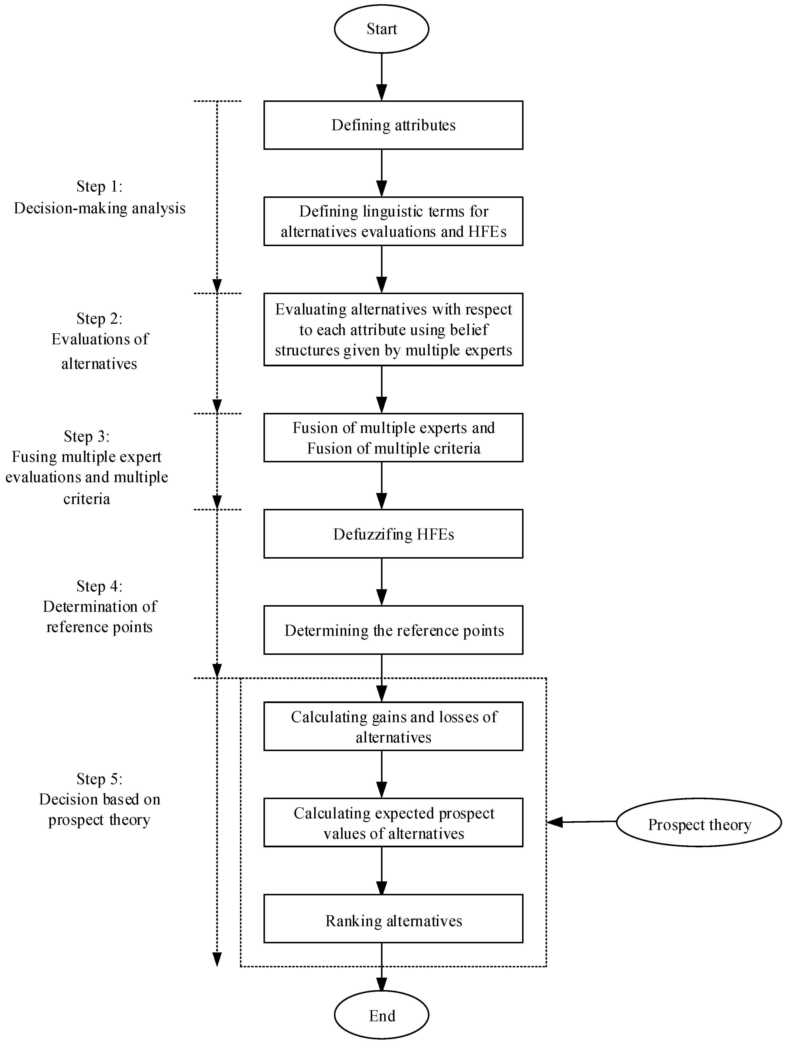
Here, a flow diagram with respect to the evidential prospect theory framework is shown in Figure 1. Specifically, the flow of the evidential prospect theory framework consists of five steps, i.e., decision-making analysis, evaluation of alternatives, fusion of evaluations, determination of reference points, and making the decision based on prospect theory, respectively.

Step 1: The task of evaluating alternatives is translated to an MCDM. Firstly, the weights of the criteria are defined. Then, for each criterion, the linguistic terms are presented.

Step 2: Evaluations of criteria for the alternatives are given by multiple domain experts. The evaluation results with respect to each criterion are characterized as a belief structure.

Step 3: In the fusion of the multiple expert evaluations, the evaluations with respect to each criterion for each alternative are combined according to the weighted average method, where the weighting factor for each evaluation is given by Equation (6). The final aggregated evaluation values for the alternatives are calculated by Equations (9) and (10).

Step 4: The HFEs are defuzzified and the reference points are determined.

Step 5: It follows from Equation (12) that the expected prospect value of each alternative will be obtained. The ranking order is presented according to the expected prospect values. That is, the most suitable alternative is chosen.

5. A Case Study

5.1. A Description of a Multiple-Criteria Decision-Making Problem

Owing to the extreme scarcity of regular fossil fuels in western China, there is a great demand for renewable energy. Renewable energy has become an indispensable part of the accelerated development of western China. A PTCSPP generates extensive power that makes it an exceptional choice for western China [39]. A renewable energy company in Beijing made plans to invest in a project involving a 50 MW PTCSPP in western China. Following the suggestions of the expert decision-making committee, there are five potential alternatives—Xinjiang Hami, Qinghai Golmud, Tibet Shigatse, Gansu Jiuquan, and Inner Mongolia Bayannur—which can be considered for the location of the PTCSPP [39]. For simplicity, Xinjiang Hami, Qinghai Golmud, Tibet Shigatse, Gansu Jiuquan, and Inner Mongolia Bayannur are labeled A₁, A₂, A₃, A₄, and A₅, respectively. Since different choices might have different benefits and different development prospects, a suitable choice must be made among the five alternatives. To make the choice, we consider the performance of each city based on three different criteria, i.e., status quo (C₁), future development (C₂), and benefits (C₃). Because this company pays more attention to potential development prospects, next to benefits, future development is the most important factor for the company. To reflect the importance of these criteria, a weight vector w = (0.25, 0.40, 0.35) was given by the renewable energy company. To choose the most desirable alternative, we introduced a group of linguistic terms, as shown in Table 1. The utilities of each linguistic term were characterized as an HFS, as shown in

Table 4. Utility functions on linguistic terms.

	VP	P	MP	M	MG	G	VG
u	{0.0,0.1}	{0.2,0.3}	{0.3,0.4}	{0.5,0.6}	{0.7,0.8}	{0.8,0.9}	{0.9,1.0}

.

5.2. Evaluations of Each Criterion for Each City

Experts gave their evaluations of each criterion for each city. The evaluation value for each criterion for each city was characterized as a belief structure, as shown in

Table 5. Evaluation values of criteria for alternatives.

City	Criterion	Expert 1	Expert 2	Expert 3	Expert 4	Expert 5
A1	C1	({MG},1.0)	({MG},1.0)	({M},0.7;{MG},0.3)	({MG},0.2;{G},0.8)	({G},1.0)
	C2	({MG},0.8;{G},0.2)	({M},1.0)	({MG},0.5;{G},0.5)	({MG},1.0)	({MP},1.0)
	C3	({M},0.7;{MG},0.3)	({MG},1.0)	({MP},0.6;{ M,MG},0.4)	({P},1.0)	({M},0.9;{MG},0.1)
A2	C1	({P},1.0)	({MP},1.0)	({M},1.0)	({MP},1.0)	({P},1.0)
	C2	({M},0.6;{ MG},0.4)	({M,MG},1.0)	({VG},1.0)	({M},1.0)	({M},1.0)
	C3	({VG},1.0)	({G},1.0)	({G},1.0)	({M},1.0)	({M},1.0)
A3	C1	({M},0.3;{G},0.7)	({M},1.0)	({M},0.8;{MG},0.2)	({M},1.0)	({M},1.0)
	C2	({M,VG},1.0)	({M},1.0)	({M},0.2;{VG},0.8)	({M},1.0)	({MG, G },1.0)
	C3	({MG},0.2;{G},0.8)	({MG},1.0)	({MG},1.0)	({G},1.0)	({MG},1.0)
A4	C1	({G},1.0)	({MG},1.0)	({MG},1.0)	({MG},1.0)	({MG},1.0)
	C2	({MP},0.2;{M,MG},0.8)	({G},1.0)	({MG},0.2;{G},0.8)	({MG,G},1.0)	({M.MG},1.0)
	C3	({G},1.0)	({MG},1.0)	({M},0.6;{ G},0.4)	({G},1.0)	({G},1.0)
A5	C1	({M},1.0)	({MG},1.0)	({MG},0.5;{G},0.5)	({G},1.0)	({G},1.0)
	C2	({M},1.0)	({M},0.3;{MG},0.7)	({MG, G},1.0)	({M},1.0)	({M,MG},1.0)
	C3	({G},1.0)	({VG},1.0)	({MG},0.8;{G},0.2)	({G},1.0)	({G},1.0)

. For example, the belief structure ({MG}, 0.7; {G}, 0.3) reflects the evaluation of A₁ given by Expert 1, wherein criterion C₃ for A₁ is medium good at a probability of 0.7 and good at a probability of 0.3.

5.3. Fusion of Evaluations

First, we focused on the fusion of the multiple expert evaluations of each city. By using the weighted average method, the evaluations were fused for each criterion, as shown in

Table 6. Aggregation of the multiple experts’ evaluations of each criterion for each city.

City	Criterion	Final Belief Structure
A1	C1	({MG}, 1.0000)
	C2	({MG}, 0.9968;{G},0.0032)
	C3	({MP}, 0.0008;{M}, 0.9095;{MG},0.0896;{G,MG}0.0001)
A2	C1	({P}, 0.5000;{MP}, 0.5000)
	C2	({M},0.9975;{MG},0.0023;{M,MG}0.0002)
	C3	({M}, 0.5000;{G}, 0.5000)
A3	C1	({M}, 1.0000)
	C2	({M}, 0.9958;{ VG}, 0.0038; {M, MG}, 0.0001;{M,VG}0.0003)
	C3	({MG}, 1.0000)
A4	C1	({MG}, 1.0000)
	C2	({M,MG},0.0420;{MG},0.4845;{G},0.4791;{MG.G}0.0016)
	C3	({G}, 1.0000)
A5	C1	({MG}, 0.0049; {G},0.9951)
	C2	({M}, 0.9458;{MG}, 0.0532,{M,MG},0.0010)
	C3	({G},1.0000)

.

For instance, evaluating city A₂ with respect to criterion C₂, the belief structures were

$$\begin{array}{l}{m}_{22}^1(\{M\})=0.6,m_{22}^1(\{MG\})=0.4;m_{22}^2(\{M,MG\})=1.0;\\ m_{23}^3(\{VG\})=1.0;m_{22}^4(\{M\})=1.0;m_{22}^5(\{M\})=1.0\end{array}$$

By Equations (3)–(8), the final belief structure was

$$m_{22}(\{M\})=0.9975,m_{22}(\{MG\})=0.0023,m_{22}(\{M,MG\})=0.0002.$$

Here, we note that others below 0.0001 were ignored since this is too small to impact on the final result. The aggregation with respect to each criterion for each city is shown in Table 6.

Then, we restricted ourselves to the fusion of multiple criteria. Evaluations of criteria for each city were fused according to the weighted average method. For example, the different belief structures with respect to each criterion for city A₂ were

$$\begin{array}{l}{m}_{21}(\{P\})=0.5000,m_{21}(\{MP\})=0.5000;\\ m_{22}(\{M\})=0.9975,m_{22}(\{MG\})=0.0023,m_{22}(\{M,MG\})=0.0002;\\ m_{23}(\{M\})=0.5000,m_{23}(\{G\})=0.5000.\end{array}$$

The weighting factors of the different belief structures for city A₂ were

w₂₁ = 0.25, w₂₂ = 0.40, w₂₃ = 0.35.

By combining Equations (9) and (10), the final aggregated weighting factor of city A₂ was as follows:

$$m_2(\{P\})=0.0089;m_2(\{MP\})=0.1238;m_2(\{M\})=0.8673.$$

Similarly, the final aggregated weighting factors for other cities are given in

Table 7. The final aggregated weighting factor for each city.

City	Final Aggregated Evaluation
A1	({M}, 0.2730; {MG}, 0.1909; {G}, 0.5361)
A2	({P}, 0.0089; {MP}, 0.1238; {M}, 0.8673)
A3	({M}, 0.9641; {MG}, 0.0359)
A4	({M}, 0.0938; {MG}, 0.8727; {G}, 0.0335)
A5	({M}, 0.4625; {MG}, 0.1685; {G}, 0.3690)

.

5.4. Decision-Making Based on Prospect Theory

First, we considered the decision matrix of the five cities and the defuzzified values based on the novel score function, as shown in

Table 8. Decision matrix of the different cities.

City	Assessment Grade	Weighting Factor	Utility Value	Defuzzified Value
A1	{M}	0.2730	{0.5, 0.6}	0.5595
	{MG}	0.1909	{0.7, 0.8}	0.7595
	{G}	0.5361	{0.8, 0.9}	0.8595
A2	{P}	0.0089	{0.2, 0.3}	0.2595
	{MP}	0.1238	{0.3, 0.4}	0.3595
	{M}	0.8673	{0.5, 0.6}	0.5595
A3	{M}	0.9641	{0.5, 0.6}	0.5595
	{MG}	0.0359	{0.7, 0.8}	0.7595
A4	{M}	0.0938	{0.5, 0.6}	0.5595
	{MG}	0.8727	{0.7, 0.8}	0.7595
	{G}	0.0335	{0.8, 0.9}	0.8595
A5	{M}	0.4625	{0.5, 0.6}	0.5595
	{MG}	0.1685	{0.7, 0.8}	0.7595
	{G}	0.3690	{0.8, 0.9}	0.8595

.

Since the reference point has an important impact on decision-making, an appropriate reference point has to be selected. The outcomes which are higher than that of the reference point are regarded as gains; the outcomes below the reference point are regarded as losses. The linguistic term “M” was regarded as the reference point, since the assessment grade “M” means that implementing the PTCSPP project in a city has bright future prospects for development at a probability of 0.5 and bad prospects at a probability of 0.5. Then, using Equation (10) the utility of each assessment grade for each city was calculated, as shown in

Table 9. Prospect value of each assessment grade for cities.

City	Assessment Grade	Weighting Factor	Gains or Losses	Prospect Value
A1	{M}	0.2730	−0.2	−0.5459
	{MG}	0.1909	0	0
	{G}	0.5361	0.1	0.1318
A2	{P}	0.0089	−0.5	−1.2226
	{MP}	0.1238	−0.4	−1.0046
	{M}	0.8673	−0.2	−0.5459
A3	{M}	0.9641	−0.2	−0.5459
	{MG}	0.0359	0	0
A4	{M}	0.0938	−0.2	−0.5459
	{MG}	0.8727	0	0
	{G}	0.0335	0.1	0.1318
A5	{M}	0.4625	−0.2	−0.5459
	{MG}	0.1685	0	0
	{G}	0.3690	0.1	0.1318

.

From Equations (12) and (13), it follows that

$$u_1^{EP}=-0.1075,u_2^{EP}=-0.6701,u_3^{EP}=-0.4659,u_4^{EP}=-0.0884,u_5^{EP}=-0.1823.$$

Thus, the ranking order of the five cities is $u_4^{EP}\succ u_1^{EP}\succ u_5^{EP}\succ u_3^{EP}\succ u_2^{EP}$, which means that city A₄ (i.e., Gansu Jiuquan) is the most desirable one.

5.5. Comparative Analysis and Discussion

Expected utility theory, as a normative theory, dominates the domain of decision-making. Thus, based on expected utility theory, the expected value of each city is

$$u_1^E=0.2730\times 0.5595+0.1909\times 0.7595+0.5361\times 0.8595=0.7585,$$

$$u_2^E=0.0089\times 0.2595+0.1238\times 0.3595+0.8673\times 0.5595=0.5321,$$

$$u_3^E=0.9641\times 0.5595+0.0359\times 0.7595=0.5667,$$

$$u_4^E=0.0938\times 0.5595+0.8727\times 0.7595+0.0335\times 0.8595=0.7441,$$

$$u_5^E=0.4625\times 0.5595+0.1685\times 0.7595+0.3690\times 0.8595=0.7039.$$

It is easy to see that the ranking order of these cities is $u_1^E\succ u_4^E\succ u_5^E\succ u_3^E\succ u_2^E$. Obviously, A₁ (i.e., Xinjiang Hami) is the most desirable city here which would be chosen to build a new manufactory.

To provide a better view of the comparison results, the ranking orders of these cities are shown in Figure 2.

From Figure 2, it is clear that the ranking orders of these cities obtained by these two approaches are remarkably different. The most desirable recommended city is A₄ (i.e., Gansu Jiuquan) based on the evidential prospect theory framework, while city A₁ (i.e., Xinjiang Hami) is the most desirable one based on expected utility theory. The main reason for this is that the result based on the evidential prospect theory framework is more in line with the actual experience of decision-makers, while the result based on expected utility theory fails to take into account DMs’ nonrational behavior. In summary, compared with these two approaches, the evidential prospect theory framework can obtain a better final decision result because it effectively captures DMs’ nonrational behavior.

6. Conclusions

Uncertain information and DMs’ nonrational behavior have received extensive attention in MCDM problems. In this paper, the evidential prospect theory framework was proposed to address MCDM problems involving hesitant and probabilistic information and nonrational behavior simultaneously. Within the proposed framework, belief structures are applied to characterize the subjective evaluations by experts of criteria for alternatives. Belief structures are fused by using a weighted average method such that the final aggregated weighting factor is determined. By combining prospect theory with belief structures, the ranking order of alternatives is determined, which can identify the most desirable alternative. The evidential prospect theory framework provides a simple and general method for MCDM problems involving hesitant and probabilistic information and nonrational behavior simultaneously. The evidential prospect theory framework proposed in this paper has two advantages: First, it makes use of evidence theory to model the various types of uncertainty in the decision-making process. Here, belief structures are applied to characterize experts’ subjective assessments of criteria for alternatives, which involve hesitant and probabilistic information simultaneously. Second, the application of prospect theory takes into account DMs’ nonrational behavior in the MCDM problems, so the decision-making results are more reasonable.

Although the evidential prospect theory framework proposed in this paper can address MCDM problems involving hesitant and probabilistic information and nonrational behavior simultaneously, the proposed framework still has its limitations. In particular, the evidential prospect theory framework was proposed under the assumption that the behaviors of DMs are not influenced by others. It is very likely that this assumption is violated, since it is inevitable that each person may be influenced by others’ behaviors in the real world. Thus, solving the interaction between decision-makers in MCDM problems will be a valuable future research topic.

References

1. Zadeh, L.A. Fuzzy sets. Inf. Control 1965, 8, 338–353. [Google Scholar] [CrossRef]
2. Liu, J.; Chan, F.T.; Li, Y.; Zhang, Y.; Deng, Y. A new optimal consensus method with minimum cost in fuzzy group decision. Knowl. Based Syst. 2012, 35, 357–360. [Google Scholar] [CrossRef]
3. Zhang, X.; Deng, Y.; Chan, F.T.; Xu, P.; Mahadevan, S.; Hu, Y. IFSJSP: A novel methodology for the job-shop scheduling problem based on intuitionistic fuzzy sets. Int. J. Prod. Res. 2013, 51, 5100–5119. [Google Scholar] [CrossRef]
4. Li, J.; Wang, J.Q. Multi-criteria decision-making with probabilistic hesitant fuzzy information based on expected multiplicative consistency. Neural Comput. Appl. 2019, 31, 8897–8915. [Google Scholar] [CrossRef]
5. García-Lapresta, J.L.; del Pozo, R.G. An ordinal multi-criteria decision-making procedure under imprecise linguistic assessments. Eur. J. Oper. Res. 2019, 279, 159–167. [Google Scholar] [CrossRef]
6. Wang, Y.J. Interval-valued fuzzy multi-criteria decision-making based on simple additive weighting and relative preference relation. Inf. Sci. 2019, 503, 319–335. [Google Scholar] [CrossRef]
7. Lin, M.; Wang, H.; Xu, Z. TODIM-based multi-criteria decision-making method with hesitant fuzzy linguistic term sets. Artif. Intell. Rev. 2019, 4, 1–25. [Google Scholar]
8. Kahneman, D.; Tversky, A. Prospect Theory: An analysis of decision under risk. Econom. J. Econom. Soc. 1979, 47, 263–291. [Google Scholar] [CrossRef]
9. Quiggin, J. A theory of anticipated utility. J. Econ. Behav. Organ. 1982, 3, 323–343. [Google Scholar] [CrossRef]
10. Shalev, J. Loss aversion equilibrium. Int. J. Game Theory 2000, 29, 269–287. [Google Scholar] [CrossRef]
11. Liu, P.; Jin, F.; Zhang, X.; Su, Y.; Wang, M. Research on the multi-attribute decision-making under risk with interval probability based on prospect theory and the uncertain linguistic variables. Knowl. Based Syst. 2011, 24, 554–561. [Google Scholar] [CrossRef]
12. Peng, J.J.; Wang, J.Q.; Wu, X.H. Novel multi-criteria decision-making approaches based on hesitant fuzzy sets and prospect theory. Int. J. Inf. Technol. Decis. Mak. 2016, 15, 621–643. [Google Scholar] [CrossRef]
13. Peng, X.; Dai, J. Approaches to Pythagorean fuzzy stochastic multi-criteria decision making based on prospect theory and regret theory with new distance measure and score function. Int. J. Intell. Syst. 2017, 32, 1187–1214. [Google Scholar] [CrossRef]
14. Peng, X.; Yang, Y. Algorithms for interval-valued fuzzy soft sets in stochastic multi-criteria decision making based on regret theory and prospect theory with combined weight. Appl. Soft Comput. 2017, 54, 415–430. [Google Scholar] [CrossRef]
15. Dempster, A.P. Upper and lower probabilities induced by a multivalued mapping. Ann. Math. Stat. 1967, 38, 325–339. [Google Scholar] [CrossRef]
16. Shafer, G. A Mathematical Theory of Evidence; Princeton University Press: Princeton, NJ, USA, 1976. [Google Scholar]
17. Yang, J.B.; Liu, J.; Wang, J.; Sii, H.S.; Wang, H.W. Belief rule-base inference methodology using the evidential reasoning approach-RIMER. IEEE Trans. Syst. Man Cybern. Part A Syst. Hum. 2006, 36, 266–285. [Google Scholar] [CrossRef]
18. Wang, Y.M.; Yang, J.B.; Xu, D.L. Environmental impact assessment using the evidential reasoning approach. Eur. J. Oper. Res. 2006, 174, 1885–1913. [Google Scholar] [CrossRef]
19. Li, X.; Dai, X.; Dezert, J.; Smarandache, F. Fusion of imprecise qualitative information. Appl. Intell. 2010, 33, 340–351. [Google Scholar] [CrossRef]
20. Altınçay, H. On the independence requirement in Dempster-Shafer theory for combining classifiers providing statistical evidence. Appl. Intell. 2006, 25, 73–90. [Google Scholar] [CrossRef]
21. Guo, H.; Shi, W.; Deng, Y. Evaluating sensor reliability in classification problems based on evidence theory. IEEE Trans. Syst. Man Cybern. Part B 2006, 36, 970–981. [Google Scholar] [CrossRef]
22. Kroupa, T. Extension of belief functions to infinite-valued events. Soft Comput. 2012, 16, 1851–1861. [Google Scholar] [CrossRef]
23. Su, X.; Deng, Y.; Mahadevan, S.; Bao, Q. An improved method for risk evaluation in failure modes and effects analysis of aircraft engine rotor blades. Eng. Fail. Anal. 2012, 26, 164–174. [Google Scholar] [CrossRef]
24. Gao, C.; Wei, D.; Hu, Y.; Mahadevan, S.; Deng, Y. A modified evidential methodology of identifying influential nodes in weighted networks. Phys. A Stat. Mech. Appl. 2013, 392, 5490–5500. [Google Scholar] [CrossRef]
25. Zhang, Y.; Deng, X.; Wei, D.; Deng, Y. Assessment of E-Commerce security using AHP and evidential reasoning. Expert Syst. Appl. 2012, 39, 3611–3623. [Google Scholar] [CrossRef]
26. Xu, P.; Deng, Y.; Su, X.; Mahadevan, S. A new method to determine basic probability assignment from training data. Knowl. Based Syst. 2013, 46, 69–80. [Google Scholar] [CrossRef]
27. Liu, Z.G.; Pan, Q.; Dezert, J. A belief classification rule for imprecise data. Appl. Intell. 2014, 40, 214–228. [Google Scholar] [CrossRef]
28. Deng, X.; Hu, Y.; Deng, Y.; Mahadevan, S. Supplier selection using AHP methodology extended by D numbers. Expert Syst. Appl. 2014, 41, 156–167. [Google Scholar] [CrossRef]
29. Nusrat, E.; Yamada, K. A descriptive decision-making model under uncertainty: Combination of Dempster-Shafer theory and prospect theory. Int. J. Uncertain. Fuzziness Knowl. Based Syst. 2013, 21, 79–102. [Google Scholar] [CrossRef]
30. Liou, J.J.; Chuang, Y.C.; Zavadskas, E.K.; Tzeng, G.H. Data-driven hybrid multiple attribute decision-making model for green supplier evaluation and performance improvement. J. Clean. Prod. 2019, 241, 1–12. [Google Scholar] [CrossRef]
31. Phochanikorn, P.; Tan, C. An Integrated Multi-Criteria Decision-Making Model Based on Prospect Theory for Green Supplier Selection under Uncertain Environment: A Case Study of the Thailand Palm Oil Products Industry. Sustainability 2019, 11, 1872. [Google Scholar] [CrossRef]
32. Yong, D.; WenKang, S.; ZhenFu, Z.; Qi, L. Combining belief functions based on distance of evidence. Decis. Support Syst. 2004, 38, 489–493. [Google Scholar] [CrossRef]
33. Jousselme, A.L.; Grenier, D.; Bossé, É. A new distance between two bodies of evidence. Inf. Fusion 2001, 2, 91–101. [Google Scholar] [CrossRef]
34. Tversky, A.; Kahneman, D. Advances in Prospect Theory: Cumulative representation of uncertainty. J. Risk Uncertain. 1992, 5, 297–323. [Google Scholar] [CrossRef]
35. Torra, V. Hesitant fuzzy sets. Int. J. Intell. Syst. 2010, 25, 529–539. [Google Scholar] [CrossRef]
36. Xia, M.M.; Xu, Z.S. Hesitant fuzzy information aggregation in decision making. Int. J. Approx. Reason. 2011, 52, 395–407. [Google Scholar] [CrossRef] [Green Version]
37. Zhang, X.; Xu, Z. The TODIM analysis approach based on novel measured functions under hesitant fuzzy environment. Knowl. Based Syst. 2014, 61, 48–58. [Google Scholar] [CrossRef]
38. Farhadinia, B. A Novel Method of Ranking Hesitant Fuzzy Values for Multiple Attribute Decision-Making Problems. Int. J. Intell. Syst. 2013, 28, 752–767. [Google Scholar] [CrossRef]
39. Wu, Y.; Zhang, B.; Wu, C.; Zhang, T.; Liu, F. Optimal site selection for parabolic trough concentrating solar power plant using extended PROMETHEE method: A case in China. Renew. Energy 2019, 143, 1910–1927. [Google Scholar] [CrossRef]
Figure 1. A flow diagram of the evidential prospect theory framework.
Symmetry 11 01467 g001
Figure 2. The ranking orders of cities.
Symmetry 11 01467 g002