Abstract
In cryptography, the property of randomness in pseudo-random generators is very important to avoid any pattern in output sequences, to provide security against attacks, privacy and anonymity. In this article, the randomness of the family of sequences obtained from the generalized self-shrinking generator is analyzed. Moreover, the characteristics, generalities and relationship between the t-modified self-shrinking generator and the generalized self-shrinking generator are presented. We find that the t-modified self-shrunken sequences can be generated from a generalized self-shrinking generator. Then, an in-depth analysis of randomness focused on the generalized sequences by means of complete and powerful batteries of statistical tests and graphical tools is done, providing a useful vision of the behaviour of these sequences and proving that they are suitable to be used in cryptography.
1. Introduction
In cryptography, randomness plays an important role in multiple and diverse applications. Random numbers are employed to generate cryptographic keys, challenges, nonces, to encrypt messages and at different steps of cryptographic algorithms and protocols [1,2,3,4].
A pseudo-random number generator is an algorithm for creating a sequence of numbers that is supposed to be indistinguishable from a uniformly chosen random sequence. The sequence is not really random, since it is completely determined by a small set of initial values, called the seed. However, in cryptography, where the security of many cryptographic schemes lies in the quality of pseudorandom generators, it is necessary that the sequences meet the following requirements—(1) the generated sequence must not be distinguished from a truly random sequence; (2) the sequence must be unpredictable; (3) the sequence period must be very large; (4) the key space must be large enough for a brute or exhaustive force attack to be impossible; (5) the design of the generator should be resistant to the specialized attacks reported in the literature.
There is no mathematical proof that ensures the randomness of a bit sequence; however, there exists a huge number of empirical tests to determine if a sequence is random enough and secure to be used in cryptography [5]. If the sequences of a generator pass the statistical tests, then this could be accepted as a generator of random sequences. Otherwise, if several tests fail, it means that the generator is not good and must be rejected. Choosing the correct number of these tests to determine whether the sequence in question can be considered random is a very difficult task since we cannot assure how many tests are needed for it. We have chosen some of those that are considered the most complete randomness tests, like the FIPS (Federal Information Processing Standard) test 140-2 [6], Diehard Battery of Tests [7], the NIST-SP-800-22 battery test [8] and other tests from the chaos theory, that were presented in References [9,10].
The Generalized Self-Shrinking Generator (GSSG) [11] is fast, easy to be implemented and generates good cryptographic sequences, so it seems suitable for its use in lightweight cryptography and, in general, in low-cost applications. However, the randomness of these sequences has never been analysed with such a complete battery of tests.
In this article, the randomness of the family of sequences obtained from the generalized self-shrinking generator is analyzed. First, the characteristics and generalities of this family of pseudorandom generators have been considered in detail. Then, an in-depth analysis of randomness focused on the generalized sequences by means of complete batteries of statistical tests was done. Tables, figures and graphical representations illustrate the obtained results.
2. Related Work
One of the most accepted designs of Pseudo-Random Number Generator (PRNG) is based on Linear Feedback Shift Registers (LFSR) because LFSRs’ sequences can have good statistical properties and their good efficiency in hardware designs. Linear feedback shift registers have been used as basic component of such PRNG but they all have been successfully cryptanalyzed by means of different attacks such as algebraic and correlation attacks, to name a few. Its main weakness is its linearity, which allows the building of a system of equations that solves the parameters used in its design [12].
To avoid these cryptanalytic attacks, new designs use non-linear operations, such as non-linear filtering and sequence decimation, for example. The shrinking generator and the self-shrinking generators are good examples of how to convert a linearly generated sequence into a non-linear one. To do that, different rules, which decimate the LFSR produced sequence in an irregular way, are used. The Shrinking Generator (SG) was firstly proposed in 1993 by Coppersmith, Krawczyk and Mansour [13] and the Self-Shrinking Generator (SSG) in 1994 by Meier and Staffelbach [14].
In Reference [15] a novel generator based on the generalized self-shrinking stream sequence generator (called F-GSS) was proposed, the sequences generated by the F-GSS were analyzed using the NIST statistical test suite, showing that it has good pseudo-random properties.
The Modified Self-Shrinking Generator (MSSG) was proposed by Kanso in Reference [16]. The study of the randomness of this generator was carried out by the NIST statistical test suite and it was demonstrated that sequences of the MSSG have better randomness properties than those of the SSG. In Reference [17] the authors present a new non-periodic random number generator based on the shrinking generator. The randomness of the sequences of the new generator was analyzed by means of Diehard battery of tests, verifying that this new design performs well in this statistical battery of tests.
Tasheva et al. in Reference [18] proposed a variant of the SSG called the p-ary Generalized Self-Shrinking Generator (pGSSG). The authors have studied its randomness using the NIST statistical test suite, later in Reference [19] the balance property of the previously proposed p-ary Generalized Self-Shrinking Generator was studied and it was shown that the generated sequences could be considered as balanced. Erkek and Tuncer in Reference [20] have implemented the SG and Alternating Step Generator on an FPGA Altera Cyclone IV board. Generated numbers in the real time were tested using the NIST statistical test suite. The results have shown that both generators have good statistical properties. In Reference [21] the authors have studied the randomness of the Self-Shrinking generator by means of the d-Monomial test. They have found that there exist some statistical dependencies on certain randomness properties of the generalized SSG and polynomial used in its design. For this reason, they recommend to take special care when choosing the polynomial for the SSG in order to the generator be cryptographically secure. In Reference [22] the author have analyzed a keystream produced by Generalized Shrinking Multiplexing Generator controlled by Ternary m-sequences (GSMG-3m). For randomness analysis they use the NIST statistical test suite, the spectral test and, approximate entropy test. The authors have presented some cryptanalytic work of the proposed generator that prove that GSMG-3m is more secure than the Shrinking Generator.
As can be seen, there are few works that have deeply studied the randomness of the sequences generated by the different families of shrinking generators through several statistical test batteries such as those presented in this paper.
3. Preliminaries
In order to the work be self-contained, some basic concepts concerning binary sequences as well as sequence generators based on irregular decimation are introduced. All of them will be used throughout the paper.
As has been said previously, the security of many cryptographic algorithms is based on a well designed random and pseudorandom generators. It is worth mentioning that the design of reliable and secure pseudorandom number generators is an open problem and an intensive field of research in cryptography nowadays [23,24,25,26,27,28]. The family of shrinking generators is one of the most analyzed PRNG in the literature due to its performance and security when it is well designed [4,21,22,29,30,31].
3.1. PN-Sequences
Let be the Galois field. Consider a binary sequence with , for We say the sequence is periodic if there exists an integer T, called period, such that , for all . In the sequel, all the sequences considered will be binary sequences and the symbol + will denote the Exclusive-OR (XOR) logic operation.
Let r be a positive integer and let be constant coefficients with . A binary sequence satisfying the relation:
is called a (r-th order) linear recurring sequence (LRS) in . The terms are referred to as the initial terms and define the construction of the sequence uniquely.
The monic polynomial:
is called the characteristic polynomial of the linear recurring sequence and is said to be generated by .
Linear recurring sequences can be generated using Linear Feedback Shift Registers (LFSRs) [5,12,32]. In fact, an LFSR can be defined as an electronic device with r memory cells (stages) with binary content. At every clock pulse, the binary element of each stage is shifted to the adjacent stage as well as a new element is computed through the linear feedback to fill the empty stage (see Figure 1). The LFSR has maximal-length if the characteristic polynomial of the LFSR is primitive. Its output sequence is called PN-sequence (Pseudo-Noise sequence) and has period , see Reference [32].
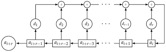
Figure 1.
LFSR of length r.
The linear complexity, , of a sequence is defined as the length of the shortest LFSR that generates such a sequence or, equivalently, as the lowest order linear recurrence relationship that generates such a sequence.
In cryptographic terms, the linear complexity must be as large as possible as defines the minimum piece of the sequence needed to get the whole sequence.
A simple result that will be useful in the next section is introduced below.
Lemma 1.
Let be a PN-sequence with period T. Then, the sequence such that is again a PN-sequence with the same period T iff .
Proof.
The sequence is a PN-sequence iff , see Reference [32] (pag. 78). The sequences for are shifted versions of with different starting points. If we XOR a PN-sequence with a shifted sequence of itself, then we have the same PN-sequence but starting at a different bit [32] (Theorem 4.3–4.5). Thus, is the same sequence as except for the starting point, that is, where is a positive integer. □
3.2. Modified Self-Shrinking Generator (MSSG)
Decimation is a very habitual technique to produce pseudo-random sequences with cryptographic applications [33,34]. In practice, the underlying idea in this kind of generators is the irregular decimation of a PN-sequence according to the bits of another.
The Modified Self-Shrinking Generator (MSSG) introduced by Kanso in Reference [16] is a modification of the well-known Self-Shrinking Generator (SSG) [14]. Indeed, in the MSSG the PN-sequence generated by a maximal-length LFSR is self-decimated. The decimation rule is very simple and can be described as follows: given three consecutive bits , , the output sequence is computed as
The output sequence is known as the Modified Self-Shrunken sequence (MSS-sequence). If L is the length of the maximal-length LFSR that generates , then the linear complexity of the corresponding MSS-sequence satisfies:
and the period T of the sequence, when L is odd, satisfies:
as proved in Reference [16]. As usual, the key of this generator is the initial state of the LFSR that generates . The characteristic polynomial of such a register is also recommended to be part of the key.
Example 1. 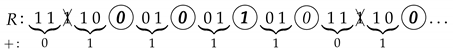
Consider the LFSR of length with characteristic polynomial and the initial state . The corresponding PN-sequence is given by with period .
The MSS-sequence is obtained as follows:
The obtained sequence (encircled bits) has period and it can be checked that its characteristic polynomial is . Thus, the linear complexity of this MSS-sequence is .
In Reference [30], the authors showed that the sequences produced by this generator are contained in the family of sequences generated by the generalized self-shrinking generator.
3.3. The Generalized Self-Shrinking Generator (GSSG)
In this subsection, we introduce the most representative generator in this family of decimation-based sequence generators, that is, the Generalized Self-Shrinking Generator (GSSG) [11]. In fact, the sequences produced by this generator include the sequences produced by the generators previously described.
Let be an PN-sequence produced by a maximal-length LFSR with L stages. Let be an L-dimensional binary vector and a sequence defined as: . For , the decimation rule is defined as follows:
The output sequence generated associated with G, denoted by , is called the Generalized Self-Shrunken sequence (GSS-sequence).
When G ranges over , then corresponds to the possible shifts of , that is, the sequence is a shifted version of the PN-sequence . Moreover, we obtain the family of generalized self-shrunken sequences based on the PN-sequence given by the set of sequences denoted by . In Table 1, the algorithm to compute these sequences is shown (Algorithm 1).

Table 1.
Algorithm to compute the GSS-sequences.
Example 2.
Consider the primitive polynomial and the corresponding PN-sequence . We can construct the GSS-sequences shown in Table 2. The underlined bits in the different sequences are the digits of the corresponding sequences. The PN-sequence is written at the bottom of the table.
Table 2.
Family of Generalized Self-Shrunken sequences generated by .
4. The t-Modified Self-Shrinking Generator
A generalization of GSSG, the t-Modified Self-Shrinking Generator (t-MSSG) was introduced by Cardell et al. in Reference [31] and can be described as follows. Consider a maximal-length LFSR with L stages that generates the PN-sequence . The t-modified self-shrinking generator, with , can be constructed making use of a very simple decimation rule.
Given t consecutive bits of the PN-sequence, the output sequence of this generator is known as the t-Modified Self-Shrunken sequence (t-MSS-sequence) and computed as follows:
Notice that the value gives rise to the self-shrinking generator [14] while the value defines the modified self-shrinking generator. In Table 3 the algorithm to compute this sequence is presented (Algorithm 2). Characteristics and generalities of the t-MSS-sequences can be found in Reference [31].
Table 3.
Algorithm to compute the t-MSS-sequence.
Relationship between t-Modified Self-Shrunken Sequences and Generalized Self-Shrunken Sequences (GSS-Sequences)
Now, we analyse the close relationship between t-Modified Self-Shrunken sequences (t-MSS-sequences) and Generalized Self-Shrunken sequences (GSS-sequences).
In Theorem 1 of Reference [30], they analyse the relationship between modified self-shrunken sequences and generalized self-shrunken sequences with a result similar to the following:
Theorem 1.
The t-MSS-sequence as a result of self-decimating a PN-sequence with characteristic polynomial of degree L and , can be generated from a generalized self-shrinking generator with a primitive polynomial of the same degree L.
Proof.
Let be a PN-sequence with characteristic polynomial of degree L which is self-decimated. In order to generate the t-MSS-sequence, sets of t bits , have to be taken. Applying the decimation rule defined in 2, if , the bit is kept. Otherwise, it is discarded. According to Lemma 1, the sequence defined as is obtained by decimating the sequence by distance t.
Since , according to Reference [32], we have that is a PN-sequence generated by a primitive polynomial of the same degree, L.
Also, if the sequence is taken, with , this means that the sequence is being decimated again by the distance t. As before, we have that is also a PN-sequence with primitive polynomial [32].
In order to obtain the t-MSS-sequence, the t-MSSG decimation rule is applied to the sequences and . As both sequences are shifted versions of the PN-sequence , we can generate such a t-MSS-sequence by a GSSG with characteristic polynomial . □
As a result of the previous theorem, we have that:
Corollary 1.
If , then the t-MSS-sequence is generated as a generalized sequence with the same primitive polynomial .
Proof.
It follows from the following idea: the sequence is a shifted version of the PN-sequence when , see Reference [32] (pag. 76). □
The next theorem gives us the primitive polynomial that we need in Theorem 1 in order to the GSSG generates the t-MSS-sequence obtained with a characteristic polynomial .
Theorem 2.
When , the primitive polynomial in Theorem 1 is:
where is a root of .
Proof.
The primitive polynomial can be expressed as:
where is a primitive element in such a field as well as a root of . Furthermore, any element of the PN-sequence is obtained as:
with [35]. When , it is said that the PN-sequence is in its characteristic phase.
The following sequence is obtained:
decimating the sequence by distance t. That is a PN-sequence (since ) and each one of its bits can be computed as:
If and , then any element of the PN-sequence can be computed as follows:
Therefore, the characteristic polynomial of the PN-sequence is,
or, equivalently,
□
Lemma 2.
Given a PN-sequence of prime period and characteristic polynomial of degree L, then sequence is a PN-sequence of period T, for any t.
Proof.
According to Reference [32], is a PN-sequence of period T if . Since T is prime, then for any t. □
Theorem 3.
Given a PN-sequence with period prime and characteristic polynomial of degree L, then the t-MSS-sequence obtained for any t is a generalized sequence generated with a primitive polynomial of degree L.
Proof.
The proof follows the same reasoning used in Theorem 1 and Lemma 2. □
Example 3.
Given , the period of the PN-sequence is , which is a prime number. Table 4 shows all the t-MSS-sequences generated with this polynomial. All of them are generalized sequences obtained from a primitive polynomial of degree 5. It is important to mention that some generalized sequences can be generated using different primitive polynomials. For example, the generalized sequence can be obtained using any primitive polynomial of degree 5.
Table 4.
t-MSS-sequences obtained with .
Next, the relationship between t-MSS-sequences and GSS-sequences is analyzed from other point of view, using the cyclotomic cosets given in Reference [32].
Next, we introduce the concept of cyclotomic coset [32] and some of its properties:
Definition 1
(Cyclotomic cosets ). : Let . We define the equivalence relation R between as follows: if there exists an integer j, , such that
is partitioned into resultant equivalence classes called the cyclotomic cosets mod .
The smallest integer i in any equivalence class is defined as the leader of the coset and is denoted by . The cardinal of a coset is L or a proper divisor of L. The characteristic polynomial of a cyclotomic coset is the polynomial , where the degree r equals the cardinal of the coset and is a root of the LFSR characteristic polynomial.
Following [32] (Chapter 4), is a proper coset if , therefore in this case, is a primitive polynomial, which is a remarkable property because if is a primitive polynomial the sequence generated by the basic LFSR is as large as possible.
Example 4.
Consider the set . Notice that is a primer integer. There are six cyclotomic cosets given by:
In this case, all cosets are proper cosets and have cardinal 5. If is considered the characteristic polynomial of the LFSR, then the corresponding characteristic polynomial of the cosets are given in Table 5. Since all cosets are proper, all the characteristic polynomials are primitive of degree 5.
Table 5.
Characteristic polynomial of cyclotomic cosets.
Theorem 4.
Consider a PN-sequence of period prime and its characteristic polynomial of degree L, then both t-MSS-sequences obtained for any and are generalized sequences produced by the same polynomial of degree L iff and belong to the same coset.
Proof.
According to the proof of Theorem 1, a t-MSS-sequence is obtained decimating the sequence with a shifted version of itself, that is, as a generalized sequence. According to [32] (Theorem 5.5), and are shifted versions of the same PN-sequence iff and belong to the same coset. Thus, the decimation rule is applied to two shifted versions of the same PN-sequence and, consequently, a generalized sequence has been generated. □
As already mentioned, Table 4 shows all the t-MSS-sequences generated by and . Notice that when and are in the same coset, then the corresponding t-MSS-sequences are generalized GSS-sequences produced by the same polynomial (characteristic polynomial of the LFSR).
Furthermore, reciprocal polynomials generate sometimes the same sequences with different starting points. For example, the generalized sequence produced with can be also generated as a generalized sequence using .
In the following example (Example 5), notice that when is not prime, different types of cyclotomic cosets can be obtained [31].
Example 5.
Consider the set . Notice that is not a prime number. There are 4 cyclotomic cosets given by:
In this case, and are proper cosets and and are improper cosets. Therefore, we know that the and are primitive polynomials. Consider as the characteristic polynomial of the LFSR. Then, the characteristic polynomial of the cosets are given in Table 6. We can check that and are primitive polynomials of degree 4 and is an irreducible polynomial of degree 4. The polynomial is a primitive polynomial of degree 2.
Table 6.
Characteristic polynomial of cyclotomic cosets.
Theorem 5.
Given a PN-sequence of period and characteristic polynomial of degree L, then both t-MSS-sequences obtained for any and are GSS-sequences generated by the same primitive polynomial of degree L iff and belong to the same proper coset.
Proof.
If the coset , such that is proper, it means that . The rest follows from previous results. □
Remark 1.
When , the corresponding t-MSS-sequence is a generalized sequence iff is a primitive polynomial of degree equal to (cardinal of ).
Since, under not very restrictive conditions, the GSS-sequences include the other sequences produced by decimation-based generators, our randomness analysis focuses on this class of binary sequences.
In Table 7, we summarize the three more popular decimation-based sequence generators with the bounds for their periods and their linear complexities that were discussed in this work.
Table 7.
Summary of the main characteristics of the three decimation-based generators discussed in this work.
5. Statistical Randomness Analysis
In this section, an exhaustive analysis of randomness of the proposed GSS-sequences is presented by using different batteries of statistical tests to study their behaviour. Some graphical tools from chaos theory have been used [9,10], for example, return maps, chaos game, Lyapunov exponent, and so forth. The generator and the battery of tests were implemented with Matlab 9.1 (2017) in a Windows 10 environment in a 64 bits PC with CPU Intel Core i7-870, at 2.93 GHz.
For our study, GSS-sequences are generated from PN-sequences coming from maximal-length LFSRs with characteristic polynomials of degree less than or equal to 27. Every one of these sequences has passed perfectly the Diehard battery of tests, considered one of the most important and powerful tool for randomness study.
Furthermore, the family of GSS-sequences is analysed with the family of statistical tests FIPS 140-2, provided by the National Institute of Standards and Technology (NIST), as well as with the Lempel-Ziv Compression Test. In both cases the sequences have passed the tests.
5.1. Graphical Testing
In this section, the main graphical tests used in Reference [9], are applied to the GSS-sequences, from which their cryptographic properties can be analyzed.
The results obtained for GSS-sequences of length bits, is presented. These sequences are generated by the GSSG from a maximal-length LFSR with the 24-degree characteristic polynomial and whose initial state is the identically 1 vector of length 24.
The tests were performed with bit sequences. Most of the tests works associating every eight bits in an octet, obtaining sequences of samples of 8 bits; with the exception of the Linear complexity test that works with just one bit and the Chaos game that works associating the bits two by two.
Next, the results of graphical tests to study the randomness of our sequences is shown.
1. Return map
Return map [10] tries to measure visually the entropy of the sequence, that is, allows to detect the existence of some useful information about the parameters used in the design of pseudo-random generators [36]. This test, that customarily is used in theory of dynamic systems, is also a powerful tool in cryptanalysis.
Basically, it consists of a graph of the points of the sequence as a function of and, under certain conditions, allows us to obtain the value of the parameters of a pseudo-random sequence, defeating the security of the cryptosystem under analysis. The result should be a distribution of points where you cannot guess neither trends, nor figures, nor lines, nor symmetry, nor patterns.
Figure 2 shows the return map of our GSS-sequence as a disordered cloud, which does not provide any useful information for its cryptanalysis.
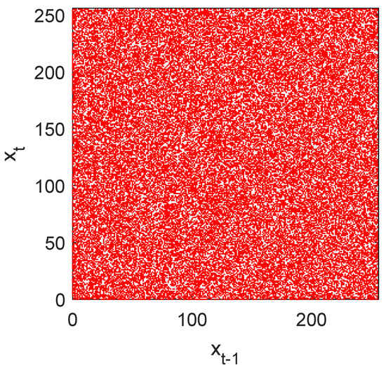
Figure 2.
Return map of GSS-sequence of bits. It provides no information about the parameters of the generator.
Figure 3a,b are the return applications of two imperfect generators where the lack of randomness can be neatly observed. Indeed, these maps present clear patterns that permit to determine the generator function and the parameter values.
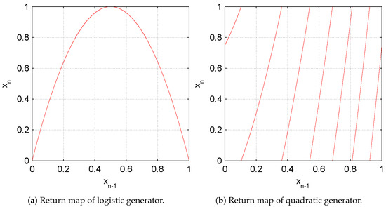
Figure 3.
Return maps of imperfect generators. The parameter values can be deduced by inspection of the return map.
2. Linear Complexity
The linear complexity () is considered as a measure of the unpredictability of a pseudo-random sequence and is a widely used metric of the security of a keystream sequence [37]. We have used the Berlekamp-Massey algorithm [38] to compute this parameter. If the characteristic polynomial of the LFSR is primitive [32], then it is known as maximal-length LFSR; moreover, its output sequence has period , where L is the degree of the characteristic polynomial.
must be as large as possible, that is, its value has to be very close to half the period [39], . From Figure 4a, it can be deduced that the value of the linear complexity of the first 20,000 bits of the sequence is just half its length, 10,000 and, from Figure 4b is observed that is irregularly close to the -line, being l the length of the sequence.
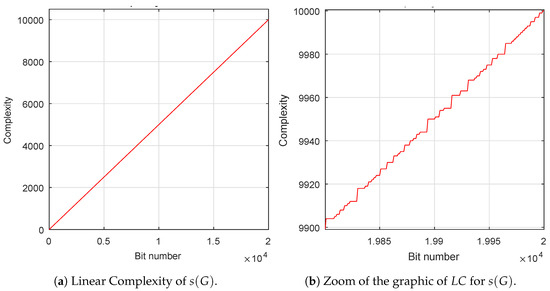
Figure 4.
Linear Complexity of for the first 20,000 most significant bits..
3. Shannon Entropy and Min-Entropy
The entropy of a sequence is defined as a measure of the amount of information of a process measured in bits or as a measure of the uncertainty of a random variable. From these two possible interpretation, the quality of the output sequence or the input of a random number generator can be described, respectively.
Shannon’s entropy is measured based on the average probability of all the values that the variable can take. A formal definition can be presented as follows,
Definition 2.
Let X be a random variable that takes on the values . Then the Shannon’s entropy is defined as
where Pr(·) represents probability.
If the process is a sequence of integers modulo m perfectly random, then its entropy is equal to n. As in the case at hand , the entropy of a random sequence must be close to bit per octet.
The min-Entropy is only measured based on the probability of the more frequent occurrence value of the variable. It is recommended by the NIST SP B standard for True Random Number Generators (TRNG).
In order to determine if the proposed generator is considered perfect from these entropies values, according to Reference [40] for a sequence of octets, it must obtain a Shannon entropy value greater or equal than bits per octet and a min-entropy greater or equal to bits per octet. In this case the following values are obtained:
then, it can be considered that this generator is correct using entropies. Note that the Shannon’s entropy value of bits per octet fits close to the theoretical perfection of 8 bits per octet.
| Shannon entropy (measured) | = | bits per octet. |
| Min-entropy (measured) | = | bits per octet, |
4. Lyapunov exponent
Lyapunov exponent measures the rate of divergence of nearby trajectories, which is a key component of chaotic dynamics. It is used as a quantitative measure for the sensitive dependence on initial conditions. It is desirable that two very close initial conditions (for instance, seeds or keys) provide very different trajectories (sequences). If Lyapunov exponent is greater than zero, the distance between two close initial conditions rapidly increases in the time, which means there exists an exponential divergence of the trajectories of a chaotic system. This value gives an idea of how different are the sequences generated by similar seeds, a very important feature to avoid attacks on the key of the generator. So, Lyapunov exponent is, in this case, a useful tool to evaluate the key space.
Next, a formal definition of Lyapunov exponent [41] is given.
Definition 3.
Consider the measure of the initial distance between two sequences and the measure of the distance between the same sequences but after t iterations. We define Lyapunov exponent as:
If , the sequences decrease their distance, tend to join and confused in one. The system converges and it is not at all random. If , the distance increases, there is dependence sensitive to initial conditions, there is an exponential divergence of the orbit and randomness grows as higher is the value of .
Note that the Lyapunov exponent uses the natural logarithm of the Euclidean distance. Nevertheless, in information theory, other type of distances for measuring the distance between two sequences are used, for example Hamming distance, which indicates the number of bit positions in which both sequences differ.
If the Lyapunov exponent is modified simply by using the Hamming distance instead of the logarithm of the Euclidean distance, then it is called the Lyapunov Hamming exponent (LHE). If two numbers are identical, then its LHE value will be 0. Nevertheless, if all the bits of both numbers are different, then its LHE will be , where n is the number of bits with which the numbers are encoded.
Obtaining the Lyapunov Hamming exponent for the chosen sequence is done by calculating the average of the LHE between every two consecutive numbers of the sequence. The best value will be .
For this case, the best value is 4; we show the value obtained for our particular sequence analyzed:
hence, the proposed generator passes perfectly this test.
| Lyapunov Hamming exponent, ideal | = | 4. |
| Lyapunov Hamming exponent, real | = | 4. |
| Absolute deviation from the ideal | = |
5. Samples in increasing order
The samples of 8 bits are ordered by increasing value and are represented by a graph. They should give a continuous straight line (red), with an inclination of 45 degrees, which must cover the blue reference line.
This representation means that all the numbers are generated (if it is continuous) and that the density is uniform (if its inclination is 45 degrees). In Figure 5a, we observe that the samples are perfectly represented by a continuous straight line with the perfect inclination of 45 degrees.

Figure 5.
Samples ordered by increasing value.
From Figure 5b, the deviation between the increasing samples is analysed and the values or 1 are obtained.
6. Chaos game
Chaos game is a method that allows converting a one-dimensional sequence into a two dimensions sequence providing a very provocative visual representation, which reveals some of the statistical properties of the sequence under study. From this graphical technique is easy to look for, visually, patterns in the sequences generated by a random number generator. Furthermore, it allows us to find non-randomness within pseudo-random sequences.
Chaos game can be described mathematically by an Iterated Functions System (IFS) [10,42,43] and through which the transition to chaos associated with fractals can be studied. The result of chaos game is called attractor and not always is a fractal, it may be any compact set. If the output is a graph with fractals or patterns, then it means that the sequence cannot be considered random.
In Figure 6, it cannot be observe any pattern or fractal, it is a messy (or unordered) cloud of points, which does not provide any useful information for analysis, which implies good randomness.
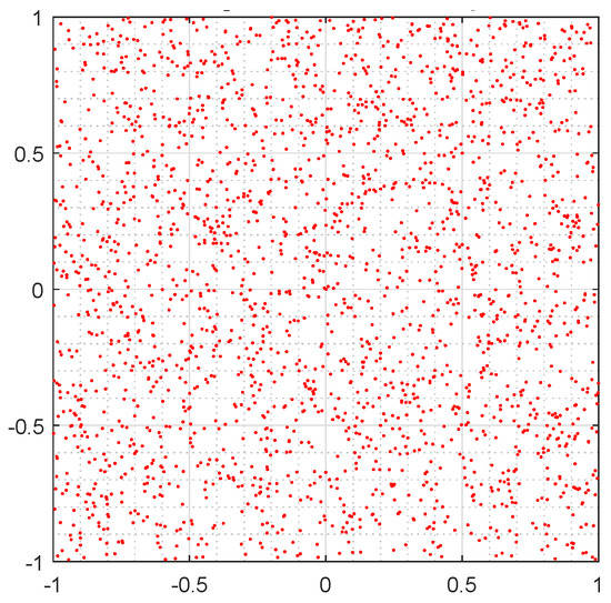
Figure 6.
GSS generator Chaos game.
In order to better understand this graphical test, we present in Figure 7a,b two Chaos Game representations, which appeared in Reference [10], which are not cryptographically secure. Their graphics are fractal which indicates that the design depends on a pattern (denoting the lack of randomness) and it is also worth mentioning that this pattern could be used to obtain important information for cryptanalysis.
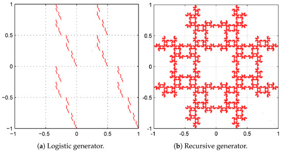
Figure 7.
Chaos game representations of imperfect generators. The observed patterns indicate a lack of randomness in the sequence.
7. Autocorrelation
The analysis of autocorrelation is a mathematical tool for finding repeating patterns analysing different sections of a message and compares them to find similarities. The autocorrelation function is defined as the crosscorrelation of the sequence with itself and allows measuring the linear relationship between random variables of processes separated a certain distance. It is very useful for finding periodic patterns within a signal.
Figure 8 represents the autocorrelation index of our GSS-sequence, for all samples available. It can be seen that the sequence has a very long period, larger than the size of the sequence analyzed since the repetition frequency is not reached in the graph.
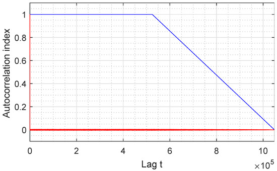
Figure 8.
Autocorrelation function of a GSS-sequence.
The first autocorrelation coefficient is always equal to 1, while the other coefficients must have the smallest possible amplitude so that the sequence can be considered random before finding the period in which it begins to repeat itself. In the case at hand, values close to 0 are obtained, which means that the proposed sequence can be considered random for this study.
8. Fast Fourier Transform
The goal of Fast Fourier Transform test is the peak heights in the discrete Fast Fourier Transform. It consists of detecting repetitive patterns in the sequence analysed which would indicate a deviation from the assumption of randomness [8].
If the sequence is random, then all the maximum harmonics of Fast Fourier Transform have approximately the same horizontal level without an up or down trend.
Figure 9 shows that all amplitude values are included in the same range, which means that the test is passed.
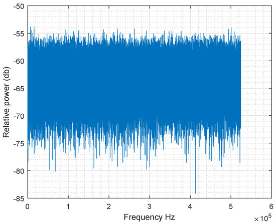
Figure 9.
Fast Fourier Transform of s(G).
9. Distribution of identical samples
In this subsection, the distance of occurrence between samples of equal value is studied, because this measure is an important property of random sequences. The most probable distance between two identical samples of a perfect sequence is zero. If this distance increases, then the probability of coincidence between the two identical samples decreases following a Poisson distribution.
Figure 10 shows that the distribution of samples of the proposed sequence is close to the ideal.
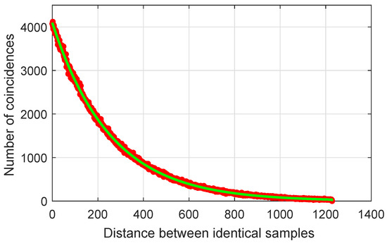
Figure 10.
Distribution of samples with equal values a function of their distance: GSS-sequence (red) and a perfect random sequence (green).
10. Collisions of the sequence
Collisions are an intrinsic property of random sequences. If one has a sequence of integers module m, the amount of different integer numbers will be m. When a number appears repeated, we say that a collision has occurred. In Reference [44] an analysis of the collisions problem is presented based on the birthday paradox which states that in a group of k people chosen at random, at least a pair of them will have the same birthday with probability:
where m is the number of days of the year and k is the number of people in the living room.
This paradox can be applied to hash functions. One of the desirable properties of cryptographic hash functions is that it is computationally impossible for a collision to occur; that is, given two different inputs, hash function does not produce the same output.
Suppose that we have a hash function of n bits, so we have output possible values. From this idea, it can be deduced the inequality:
which provides an estimated value of the quantity k of rolls of a random sequence that must be extracted to have a probability of a first collision greater than or equal to .
From Equation (3) it can be deduced the collision probability density distribution as a function of k,
In Figure 11 is represented the first collision probability density distribution function for a sequence of octets, that is, , as a red line. It can be seen that the mode of the distribution is and for a quantity of rolls the collision probability density is practically zero.
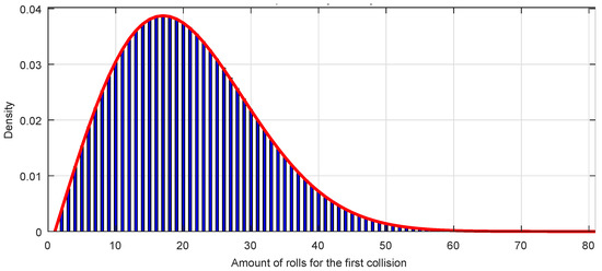
Figure 11.
Distribution of the first collisions (blue bars) and collision probability density distribution function (red line).
Any sequence with a perfect randomness must fit the first collision probability density distribution function corresponding to Equation (4).
The Figure 11 represents also a bar graph, with one bar for each value of k, of a GSS-sequence of octets. It can be seen the perfect fitting with the expected theoretical distribution.
As a curiosity, the first collision probability density distribution function coincides with a Weibull distribution function for the variable k, that is, the distribution which is most used to model data from reliability against catastrophes; in the present case, it models the amount of random number generation rolls needed for a first collision to appear, which is also a catastrophe for a hash function.
5.2. Diehard Battery of Tests
Diehard battery of tests [7] is a reliable standard and a powerful instrument for practical evaluation of the randomness of sequences of pseudo-random number generators. This tool is the first step in the evaluation process of cryptographic primitives. It cannot guarantee if your generator can be considered perfectly random, but if it does not pass the test suite, then it is not suitable for cryptographic applications.
Diehard battery consists of 15 different independent statistical tests, some of them repeated but with different parameters. The Diehard tests employ chi-squared goodness-to-fit technique to calculate a p-value, which should be uniform on if the input file contains truly independent random bits. It is considered that a bit stream really fails when it is gotten p-values of 0 or 1 to six or more places.
The GSS-sequences with characteristic polynomial of degree have passed all tests in the Diehard battery. In Table 8 we show the results obtained with the Diehard battery from a sequence with characteristic polynomial .
Table 8.
Diehard battery of tests results for a GSS sequence with characteristic polynomial of degree 27.
5.3. FIPS Test 140-2. Security Requirements for Cryptographic Modules
FIPS (Federal Information Processing Standard) Publication 140-2, is a U.S. government computer security standard [6] used to approve cryptographic modules. The National Institute of Standards and Technology (NIST) issued the FIPS 140-2 publication series to coordinate the requirements and standards for cryptography modules that include both hardware and software components (last updated 2002).
In FIPS 140-2 there are 4 statistical random number generator tests—The Monobit Test, The Poker Test, The Runs Test and The Long Runs Test. The proposed GSS-sequences with characteristic polynomials of degree pass all these tests. Below we detail the results:
- LONG RUNS TEST(PRS): Passed. There are no runs of more than 25 equal bits.
- MONOBIT TEST(PRS): Passed. The test is passed if . Our result was: 9954.
- X= POKER TEST(PRS): Passed. The test is passed if . Our result was: .
- RUNS TEST(PRS): Passed. The test is passed if the runs (for both the runs of zeros, red line, and the runs of ones, blue line) that occur (of lengths 1 through 6) are each within the corresponding interval specified in the Figure 12 by the green line.
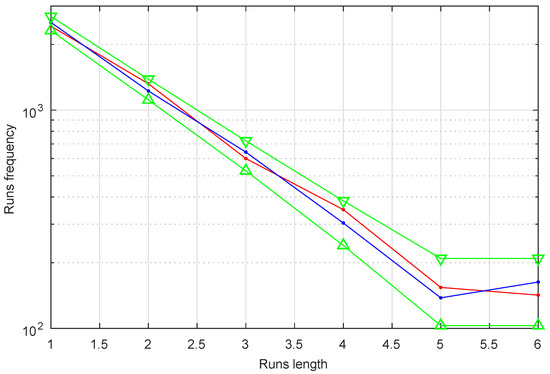 Figure 12. Run test for a GSS-sequence with characteristic polynomials of degree . Observe that the test is passed both for the runs of zeros (red line) and for the runs of ones (blue line) since they all fall within the corresponding range specified by the green line.
5.4. Lempel-Ziv Compression Test
The goal of this test is the number of cumulatively distinct patterns in the sequence. This test consists of determining how much is possible to compress the analysed sequence. If the sequence can be significantly compressed, it is considered to be non-random. The proposed GSS-sequences with characteristic polynomials of degree , pass this test with perfect results.
As can be seen throughout this section, the analyzed generator meets all the requirements needed to be used in the field of cryptography, according to points 1–4 mentioned in Section 1. Further work would be to study the resistance of this generator against the cryptographic attacks reported in the literature (Section 1, point 5).
6. Conclusions
In this article, we have found a relationship between two families of binary sequences belong to the class of decimation-based sequence generators, that is, the t-modified self-shrunken sequences can be generated from a generalized self-shrinking generator. We have analysed this relationship from two different points of view—one of them as binary sequences and other using the cyclotomic cosets. Furthermore, we have considered one of the most complete statistical test batteries for the study of randomness of sequences generated by the GSSG. In addition, we have reviewed some important graphical tests and basic and recent individual randomness tests found in the cryptographic literature. From the study of the last section, we can conclude that our random number generator (GSSG) produces good pseudo-random sequences since all the family of the sequences generated with characteristic polynomials of degree less than or equal to 27 pass satisfactorily the most important batteries of tests. The obtained results confirm the potential use of the generalized self-shrunken sequences for cryptographic purposes.
With regard to future work on this subject, the concatenation of GSS sequences from different primitive polynomials of different degrees could be analysed and studied, as well as the resistance of this generator against cryptographic attacks reported in the literature. Another important future work would be to do a comparative study of our generator with other well-known generators used in cryptographic applications nowadays.
Author Contributions
All the authors have equally contributed to the reported research in conceptualization, methodology, software and manuscript revision.
Funding
This research received no external funding.
Acknowledgments
This research has been partially supported by Ministerio de Economía, Industria y Competitividad (MINECO), Agencia Estatal de Investigación (AEI), and Fondo Europeo de Desarrollo Regional (FEDER, UE) under project COPCIS, reference TIN2017-84844-C2-1-R, and by Comunidad de Madrid (Spain) under project CYNAMON (P2018/TCS-4566), also co-funded by FSE and European Union FEDER funds. The first author was supported by CAPES (Brazil). The second author was partially supported by Spanish grant VIGROB-287 of the Universitat d’Alacant. We would like to thank Fausto Montoya for his help with the analysis of the sequences.
Conflicts of Interest
The authors declare no conflict of interest.
References
- Bhowmick, A.; Sinha, N.; Arjunan, R.V.; Kishore, B. Permutation-substitution architecture based image encryption algorithm using middle square and RC4 PRNG. In Proceedings of the 2017 International Conference on Inventive Systems and Control (ICISC), Coimbatore, India, 19–20 January 2017; pp. 1–6. [Google Scholar]
- Wortman, P.; Yan, W.; Chandy, J.; Tehranipoor, F. P2M-based security model: Security enhancement using combined puf and PRNG models for authenticating consumer electronic devices. IET Comput. Digit. Tech. 2018, 12, 289–296. [Google Scholar] [CrossRef]
- Bikram, P.; Trivedi, G.; Jan, P.; Nemec, Z. Efficient PRNG design and implementation for various high throughput cryptographic and low power security applications. In Proceedings of the 2019 29th International Conference Radioelektronika (RADIOELEKTRONIKA), Pardubice, Czech Republic, 16–18 April 2019; pp. 1–6. [Google Scholar]
- Moufek, H.; Guenda, K.; Gulliver, T.A. A new variant of the McEliece cryptosystem based on QC-LDPC and QC-MDPC codes. IEEE Commun. Lett. 2017, 21, 714–717. [Google Scholar] [CrossRef]
- Gong, G.; Helleseth, T.; Kumar, P.V. Solomon W. Golomb–Mathematician, Engineer, and Pioneer. IEEE Trans. Inf. Theory 2018, 64, 2844–2857. [Google Scholar] [CrossRef]
- FIPS PUB 140-2. Security Requirements for Cryptographic Modules. In Federal Information Processing Standards Publication 140-2; U.S. Department of Commerce; NIST, National Technical Information Service: Springfield, VA, USA, 2001.
- Marsaglia, G. The Marsaglia Random Number CDROM including the DIehard Battery of Tests of Randomness; Florida State University: Tallahassee, FL, USA, 1995; Available online: http://www.stat.fsu.edu/pub/diehard (accessed on 3 November 2019).
- National Institute of Standards and Technology. A Statistical Test Suite for Random and Pseudorandom Number Generators for Cryptographic Applications; NIST800-22, SP 800-22Rev 1a; U.S. Department of Commerce: Gaithersburg, MD, USA, 2010.
- Orúe López, A.B. Contribución al Estudio del Criptoanálisis y Diseño de los Criptosistemas Caóticos. Ph.D. Thesis, Universidad Politécnica de Madrid, Escuela Técnica Superior de Ingenieros de Telecomunicación, Madrid, Spain, 2013. [Google Scholar]
- Orúe, A.B.; Fúster-Sabater, A.; Ferná\ndez, V.; Montoya, F.; Hernández, L.; Martín, A. Herramientas gráficas de la criptografía caótica para el análisis de la calidad de secuencias pseudoaleatorias. In Proceedings of the Actas de la XIV Reunión Espan˜ola sobre Criptología y Seguridad de la Información, RECSI XIV, Menorca, Illes Balears, Spain, 26–28 October 2016; pp. 180–185. [Google Scholar]
- Hu, Y.; Xiao, G. Generalized self-shrinking generator. IEEE Trans. Inf. Theory 2004, 50, 714–719. [Google Scholar] [CrossRef]
- Klein, A. Linear Feedback Shift Registers. In Stream Ciphers; Springer: London, UK, 2013; Chapter 2; pp. 1–13. [Google Scholar]
- Coppersmith, D.; Krawczyk, H.; Mansour, Y. The shrinking generator. In Proceedings of the 13th Annual International Cryptology Conference on Advances in Cryptology (CRYPTO ’93), Santa Barbara, CA, USA, 22–26 August 1993; Springer: Berlin/Heidelberg, Germany, 1994; pp. 22–39. [Google Scholar]
- Meier, W.; Staffelbach, O. The self-shrinking generator. In Advances in Cryptology, Proceedings of EUROCRYPT 1994; Cachin, C., Camenisch, J., Eds.; Lecture Notes in Computer Science; Springer: Berlin/Heidelberg, Germany, 1984; Volume 950, pp. 205–214. [Google Scholar]
- Dong, L.; Zeng, Y.; Hu, Y. F-gss: A novel fcsr-based keystream generator. In Proceedings of the First International Conference on Information Science and Engineering, Nanjing, China, 26–28 December 2009; pp. 1737–1740. [Google Scholar]
- Kanso, A. Modified self-shrinking generator. Comput. Electr. Eng. 2010, 36, 993–1001. [Google Scholar] [CrossRef]
- Berzina, I.; Bets, R.; Buls, J.; Cers, E.; Kulesa, L. On a non-periodic shrinking generator. In Proceedings of the 2011 13th International Symposium on Symbolic and Numeric Algorithms for Scientific Computing, Timisoara, Romania, 26–29 September 2011; pp. 348–354. [Google Scholar]
- Tasheva, A.T.; Tasheva, Z.N.; Milev, A.P. Generalization of the self-shrinking generator in the Galois Field GF(pn). Adv. Artif. Intell. 2011, 2011. [Google Scholar] [CrossRef]
- Tasheva, A.; Nakov, O.; Tasheva, Z. About balance property of the p-ary generalized self-shrinking generator sequence. In Proceedings of the 14th International Conference on Computer Systems and Technologies (CompSysTech ’13), Ruse, Bulgaria, 28–29 June 2013; ACM: New York, NY, USA, 2013; pp. 299–306. [Google Scholar]
- Erkek, E.; Tuncer, T. The implementation of asg and sg random number generators. In Proceedings of the 2013 International Conference on System Science and Engineering (ICSSE), Budapest, Hungary, 4–6 July 2013; pp. 363–367. [Google Scholar]
- Boztas, S.; Alamer, A. Statistical dependencies in the self-shrinking generator. In Proceedings of the 2015 Seventh International Workshop on Signal Design and its Applications in Communications (IWSDA), Bengaluru, India, 14–18 September 2015; pp. 42–46. [Google Scholar]
- Savova-Tasheva, Z.; Tasheva, A. Analysis of keystream produced by generalized shrinking multiplexing generator controlled by ternary m-sequence. In Proceedings of the 9th Balkan Conference on Informatics (BCI’19), Sofia, Bulgaria, 26–28 September 2019; ACM: New York, NY, USA, 2019; pp. 1–7. [Google Scholar]
- Gergely, A.M.; Crainicu, B. A succinct survey on (pseudo)-random number generators from a cryptographic perspective. In Proceedings of the 2017 5th International Symposium on Digital Forensic and Security (ISDFS), Tirgu Mures, Romania, 26–28 April 2017; pp. 1–6. [Google Scholar]
- Bikram, P.; Khobragade, A.; Sai, S.; Goswami, S.S.P.; Dutt, S.; Trivedi, G. Design and implementation of low-power high-throughput PRNGs for security applications. In Proceedings of the 2019 32nd International Conference on VLSI Design and 2019 18th International Conference on Embedded Systems, Delhi, NCR, India, 5–9 January 2019; pp. 535–536. [Google Scholar]
- Prokofiev, A.O.; Chirkin, A.V.; Bukharov, V.A. Methodology for quality evaluation of PRNG, by investigating distribution in a multidimensional space. In Proceedings of the 2018 IEEE Conference of Russian Young Researchers in Electrical and Electronic Engineering (EIConRus), Moscow, Russia, 29 January–1 February 2018; pp. 355–357. [Google Scholar]
- Dalai, D.K.; Maitra, S.; Pal, S.; Roy, D. Distinguisher and non-randomness of grain-v1 for 112, 114 and 116 initialisation rounds with multiple-bit difference in ivs. IET Inf. Secur. 2019, 13, 603–613. [Google Scholar] [CrossRef]
- Avaroglu, E.; Çavdar, T. Quantum random number generators. In Proceedings of the 2018 International Conference on Artificial Intelligence and Data Processing (IDAP), Malatya, Turkey, 28–30 September 2018; pp. 1–4. [Google Scholar]
- Zhu, S.; Ma, Y.; Li, X.; Yang, J.; Lin, J.; Jing, J. On the analysis and improvement of min-entropy estimation on time-varying data. IEEE Trans. Inf. Forensics Secur. 2019, 1. [Google Scholar] [CrossRef]
- Liu, Y.; Tong, X. Hyperchaotic system-based pseudorandom number generator. IET Inf. Secur. 2016, 10, 433–441. [Google Scholar] [CrossRef]
- Cardell, S.D.; Fúster-Sabater, A. Discrete linear models for the self-shrunken sequences. Finite Fields Their Appl. 2017, 47, 222–241. [Google Scholar] [CrossRef]
- Cardell, S.D.; Fúster-Sabater, A. The t-Modified Self-shrinking Generator. In Computational Science—ICCS 2018, Proceedings of the International Conference on Computational Science (ICCS 2018), Wuxi, China, 11–13 June 2018; Shi, Y., Fu, H., Tian, Y., Krzhizhanovskaya, V.V., Lees, M.H., Dongarra, J., Sloot, P.M.A., Eds.; Lecture Notes in Computer Science; Springer: Cham, Switzerland, 2018; Volume 10860, pp. 653–663. [Google Scholar]
- Golomb, S.W. Shift Register-Sequences; Aegean Park Press: Laguna Hill, CA, USA, 1982. [Google Scholar]
- Fúster-Sabater, A. Linear Solutions for Irregularly Decimated Generators of Cryptographic Sequences. Int. J. Nonlinear Sci. Numer. Simul. 2014, 15, 377–385. [Google Scholar] [CrossRef]
- Todorova, M.; Stoyanov, B.; Szczypiorski, K.; Kordov, K. SHAH: Hash Function based on Irregularly Decimated Chaotic Map. Int. J. Electron. Telecommun. 2018, 64, 457–465. [Google Scholar] [CrossRef]
- Lidl, R.; Niederreiter, H. Introduction to Finite Fields and Their Applications; Cambridge University Press: New York, NY, USA, 1986. [Google Scholar]
- Alvarez, G.; Montoya, F.; Romera, M.; Pastor, G. Cryptanalyzing an improved security modulated chaotic encryption scheme using ciphertext absolute value. Chaos Soliton. Fract. 2005, 23, 1749–1756. [Google Scholar] [CrossRef]
- Paar, C.; Pelzl, J. Understanding Cryptography; Springer: Berlin/Heidelberg, Germany, 2010. [Google Scholar]
- Massey, J.L. Shift-register synthesis and BCH decoding. IEEE Trans. Inf. Theor. 1969, 15, 122–127. [Google Scholar] [CrossRef]
- Rueppel, R.A. Linear Complexity and Random Sequences. In Advances in Cryptology—EUROCRYPT 1985; Pichler, F., Ed.; Lecture Notes in Computer Science; Springer: Berlin/Heidelberg, Germany, 1986; Volume 219, pp. 167–188. [Google Scholar]
- Killmann, W.; Schindler, W. AIS 20/AIS 31, A Proposal for: Functionality Classes for Random Number Generators; Bundesamt für Sicherheit in der Informationstechnik (BSI): Frankfurt am Main, Germany, 2011. [Google Scholar]
- Romera, M. Técnica de los Sistemas Dinámicos Discretos; 27 CSIC, Madrid II-C; Textos Universitarios: Madrid, Spain, 1997. [Google Scholar]
- Peitgen, H.O.; Jurgens, H.; Saupe, D. Chaos and Fractals: New Frontiers of Science; Springer: New York, NY, USA, 2004. [Google Scholar]
- Barnsley, M. Fractals Everywhere, 2nd ed.; Dover Publications, Inc.: Mineola, NY, USA, 2012. [Google Scholar]
- Cormen, T.H.; Leiserson, C.E.; Rivest, R.L.; Stein, C. Introduction to Algorithms, 2nd ed.; The MIT Press: Cambridge, MA, USA, 2001. [Google Scholar]
© 2019 by the authors. Licensee MDPI, Basel, Switzerland. This article is an open access article distributed under the terms and conditions of the Creative Commons Attribution (CC BY) license (http://creativecommons.org/licenses/by/4.0/).