On a Class of Functional Differential Equations with Symmetries

Abstract

It is shown that a class of symmetric solutions of scalar non-linear functional differential equations can be investigated by using the theory of boundary value problems. We reduce the question to a two-point boundary value problem on a bounded interval and present several conditions ensuring the existence of a unique symmetric solution.

1. Introduction and Problem Formulation

The purpose of this note is to present several conditions ensuring that a functional differential equation possessing a certain symmetry-invariance property has a symmetric solution. The motivation comes partly from previous studies on antiperiodic and more general classes of solutions (e.g., [1,2,3,4] and references therein). On the other hand, it is interesting to obtain meaningful solvability conditions in cases where the techniques specific for ordinary differential equations either cannot be easily applied or are not relevant at all. Equations with functional perturbations are interesting from many points of view (see, e.g., [5,6,7,8,9] and references therein).

The class of equations we deal with includes, in particular, equations with variable argument deviations and integro-differential equations. More precisely, we consider the general functional differential equation

$$\begin{array}{cc}\hfill u^{\prime }\left(t\right)& =\left(fu\right)\left(t\right),t\in J,\hfill \end{array}$$

(1)

where J is the closure of an unbounded interval and $f:\check{C}\left(J\right)\to L_{\mathrm{loc}}\left(J\right)$ is a mapping (generally speaking, non-linear). We choose $\check{C}\left(J\right)$ to be either $L_{\mathrm{loc}}^{\infty }\left(J\right)$ or $P{C}_{\sigma }\left(J\right)$ with a specific $\sigma$ (see (13) in the next section); the reasoning to follow is common for both versions.

In the sequel, the following notation is used: $P{C}_{\sigma }\left(J\right)$ is the Fréchet space of piece-wise continuous functions $J\to \mathbb{R}$ with possible jump discontinuities at points of a given countable set $\sigma =\{t_k:k\in \mathbb{Z}\}$ endowed with the system of seminorms ${\nu }_k\left(u\right):={max}_{-k\le j\le k}{sup}_{t\in (t_{j-1},t_j)}|u\left(t\right)|$, $u\in P{C}_{\sigma }\left(J\right)$, $k\ge 1$; $C\left(J\right)$ is the Fréchet space of continuous functions on J with the sequence of seminorms ${|u|}_k={max}_{t\in [-k,k]\cap J}|u\left(t\right)|$, $k\ge 1$, $u\in C\left(J\right)$; $L_{\mathrm{loc}}\left(J\right)$ is the Fréchet space of functions that are Lebesgue integrable over every bounded interval contained in J, with the seminorms ${\parallel u\parallel }_k={\int }_{[-k,k]\cap J}|u\left(t\right)|dt$, $k\ge 1$, $u\in L_{\mathrm{loc}}\left(J\right)$; $L_{\mathrm{loc}}^{\infty }\left(J\right)$ is the Fréchet space of locally essentially bounded functions with the seminorms ${\parallel u\parallel }_{\infty ;k}={\mathrm{ess}\sup }_{t\in [-k,k]\cap J}|u\left(t\right)|$, $k\ge 1$, $u\in L_{\mathrm{loc}}^{\infty }\left(J\right)$; $C\left(J_0\right)$ and $L\left(J_0\right)$ are, respectively, the Banach spaces of continuous and integrable functions on a bounded interval $J_0\subset J$ endowed with the standard norms.

A solution of (1) is an absolutely continuous function satisfying equality (1) almost everywhere. In what follows, we consider the case where the restriction ${f|}_{P{C}_{\sigma }\left(J\right)}$ (or directly f if $\check{C}\left(J\right)=P{C}_{\sigma }\left(J\right)$) is continuous as a mapping from $P{C}_{\sigma }\left(J\right)$ to $L_{\mathrm{loc}}\left(\tilde{J}\right)$ with some $\tilde{J}$ strictly containing J (singularities on the boundary are excluded).

We study the problem of the existence of solutions $u:J\to \mathbb{R}$ of Equation (1) possessing the symmetry property

$$\mu u\left(\psi \right(t\left)\right)=u\left(t\right),t\in J,$$

(2)

where $\mu \in \mathbb{R}\setminus \left\{0\right\}$ is a given constant and $\psi :J\to J$ is a monotone increasing, absolutely continuous function. Due to the nature of property (2), we impose throughout the paper the following symmetry condition on the operator f:

$$\mu {\psi }^{\prime }\left(t\right)\left(fu\right)\left(\psi \left(t\right)\right)=\left(fu\right)\left(t\right),t\in J,$$

(3)

for any function $u\in \check{C}\left(J\right)$ possessing property (2). We also assume that J is invariant with respect to the action of $\psi$, i.e.,

$$\psi \left(J\right)\subset J.$$

(4)

Typically, J is either $(-\infty ,\infty )$ or one of the intervals $(-\infty ,0]$, $[0,\infty )$.

In (1), (3), and all similar relations below, we assume that the corresponding relations between integrable functions are satisfied almost everywhere and do not always indicate this fact explicitly.

Condition (2) describes a class of properties of solutions such as evenness, oddness, periodicity, and antiperiodicity. For example, $\psi$ may have the form $\psi \left(t\right)=ϵt+T$, $t\in (-\infty ,\infty )$, where T is fixed and $ϵ\in \{-1,1\}$; then condition (2) defines a Floquet-type solution with $ϵ=1$ (for many-dimensional systems, solutions with this and more general properties are investigated in [1,2,3,4]), while for $ϵ=-1$, (2) describes the solutions studied in [2,10]. For more complicated functions $\psi$, the “symmetric” character of property (2) is less obvious compared to, e.g., periodicity or antiperiodicity. For example, with $\psi \left(t\right)=2t-1$ and $\mu =2^{-n}$, property (2) holds for the function $u\left(t\right)={(t-1)}^n$, $t\in \mathbb{R}$.

Note that condition (3) naturally arises in the context of the study of solutions with property (2). For example, if (1) is an ordinary differential equation of the form

$$u^{\prime }\left(t\right)=h(t,u\left(t\right)),t\in (-\infty ,\infty ),$$

(5)

then assumption (3) is satisfied when the function $h:{\mathbb{R}}^2\to \mathbb{R}$ is such that

$$\mu {\psi }^{\prime }\left(t\right)h(\psi \left(t\right),{\mu }^{-1}z)=h(t,z)$$

(6)

for a. e. $t\in (-\infty ,\infty )$ and all $z\in \mathbb{R}$. Relation (6) is a particular case of the property considered in [3] (see also the references therein for more details) for weakly non-linear systems of ordinary differential equations; it ensures the invariance of Equation (5) under the transformation $t\to \psi \left(t\right)$, $u\to \mu u$. The proof of the existence of symmetric solutions in [3] involves a small parameter argument.

In this note, we focus on a general functional differential Equation (1) and formulate several conditions guaranteeing the existence of solutions with property (1). The method is different from that employed in [3]; here, we use results from the theory of boundary value problems. Note also that (1) may involve various kinds of argument deviations, in contrast to the most frequently studied delay equations (see, e.g., [11]).

2. Extension by Symmetry

It is convenient to work with the restriction of (1) to suitable bounded intervals. Although such restrictions are, generally speaking, impossible for general equations (1) without specifying additional initial data, it turns out that, in our case, this can be done in a straightforward way due to the symmetry assumption (3). Let us fix some value $t_0\in J$ with $\psi \left(t_0\right)\ne t_0$. For definiteness, assume that $\psi \left(t_0\right)>t_0$. It is clear from the problem formulation that the restriction ${v=u|}_{[t_0,\psi \left(t_0\right)]}$ of every solution u of (1), (2) to the interval $[t_0,\psi \left(t_0\right)]$ satisfies the two-point boundary condition

$$v\left(t_0\right)=\mu v\left(\psi \left(t_0\right)\right).$$

(7)

Moreover, a converse statement, in a sense, is true under condition (3). To formulate it in a rigorous way, we introduce some notation and make the equation setting more specific.

The conditions assumed on the function $\psi$ imply that the inverse function ${\psi }^{-1}$ is well defined and the sequence of numbers $\dots <{\psi }^{-2}\left(t_0\right)<{\psi }^{-1}\left(t_0\right)<t_0<\psi \left(t_0\right)<{\psi }^2\left(t_0\right)<\dots$ is strictly increasing. At this point, it is natural to make more precise the choice of the interval J on which Equation (1) is studied under the symmetry condition (3). Namely, we assume that $t_0$ is chosen so that

$$\begin{array}{cc}\hfill \underset{k\to \infty }{lim}{\psi }^{-k}\left(t_0\right)& ={\alpha }^{-},\hfill \end{array}$$

(8)

$$\begin{array}{cc}\hfill \underset{k\to \infty }{lim}{\psi }^k\left(t_0\right)& ={\alpha }^{+}\hfill \end{array}$$

(9)

with $|{\alpha }^{-}|+|{\alpha }^{+}|=\infty$ and take

$$J:=\langle {\alpha }^{-},{\alpha }^{+}\rangle ,$$

(10)

where “〈” means, respectively, “[” or “(”, depending on whether the corresponding value at the bracket is finite or not. For example, if $\psi :t\mapsto t/2$ and $t_0=-1$, then (10) gives $J=(-\infty ,0]$.

Thus, we consider Equation (1) on the unbounded interval J of form (10). Due to the properties mentioned above, J can be represented as the union of the half-open intervals

$$I_k:=[{\psi }^k\left(t_0\right),{\psi }^{k+1}\left(t_0\right)),k\in \mathbb{Z},$$

(11)

if ${\alpha }^{+}=\infty$ and

$$I_k:=({\psi }^k\left(t_0\right),{\psi }^{k+1}\left(t_0\right)],k\in \mathbb{Z},$$

(12)

if ${\alpha }^{-}=-\infty$. It is obvious that in both cases, these intervals are mutually disjoint, which justifies the following notation: for every $t\in J$, put $j\left(t\right)$ to be equal to j, where j is such that $t\in I_j$.

In case the domain $\check{C}\left(J\right)$ for f in the problem formulation is chosen to be $P{C}_{\sigma }\left(J\right)$, from now on, we put

$$\sigma :=\{{\psi }^k\left(t_0\right):k\in \mathbb{Z}\}$$

(13)

in the definition of $P{C}_{\sigma }\left(J\right)$ appearing in the problem formulation.

Lemma 1.

If a continuous function $v:{\overline{I}}_0\to \mathbb{R}$ satisfies the two-point boundary condition (7), then the function

$$v_{\ast }\left(t\right):={\mu }^{-j\left(t\right)}v\left({\psi }^{-j\left(t\right)}\left(t\right)\right),t\in J,$$

(14)

has property (2).

Proof. 

Let $v_{\ast }:J\to \mathbb{R}$ be defined by (14). Since $\psi$ is increasing, it is clear from (11) that

$$\psi \left(I_k\right)\subset I_{k+1}$$

(15)

for any k, and hence, for $t\in I_1$, (14) yields

$$v_{\ast }\left(t\right)={\mu }^{-1}v\left({\psi }^{-1}\left(t\right)\right)={\mu }^{-1}{v}_{\ast }\left({\psi }^{-1}\left(t\right)\right).$$

Arguing by induction, we easily obtain that $v_{\ast }$ satisfies the equality

$$v_{\ast }\left(t\right)={\mu }^{-k}{v}_{\ast }\left({\psi }^{-k}\left(t\right)\right),t\in I_k,$$

(16)

for every integer k. It follows immediately from (16) that

$$\mu v_{\ast }\left(\psi \left(t\right)\right)={\mu }^{1-k}{v}_{\ast }\left({\psi }^{1-k}\left(t\right)\right)=v_{\ast }\left(t\right),t\in I_k,$$

for all k. Since ${\bigcup }_{k\in \mathbb{Z}}{I}_k=J$, this means that $v_{\ast }$ satisfies (2) on J. □

For any $v\in C\left({\overline{I}}_0\right)$, let $v_{\ast }:J\to \mathbb{R}$ stand for the corresponding function (14). Let $C_0\left({\overline{I}}_0\right)$ be the subspace of $C\left({\overline{I}}_0\right)$ constituted by the functions satisfying condition (7) (here and below, ${\overline{I}}_k$ denotes the closure of $I_k$, $k\in \mathbb{Z}$). The following statement is an immediate consequence of formula (14).

Lemma 2.

Let $v\in C\left({\overline{I}}_0\right)$. Then $v_{\ast }$ is continuous if and only if $v\in C_0\left({\overline{I}}_0\right)$. For $v\in C\left({\overline{I}}_0\right)\setminus C_0\left({\overline{I}}_0\right)$, the function $v_{\ast }\in \check{C}\left(J\right)$ has countably many discontinuities of the first kind at points of set (13).

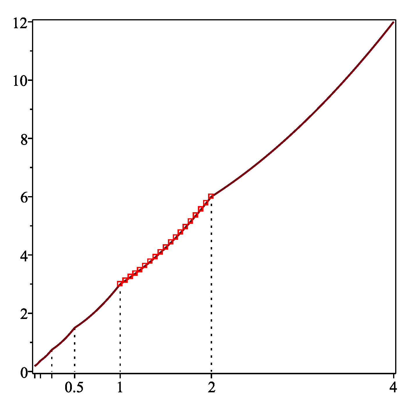
Lemma 1 is a natural generalization of the corresponding well-known statements for ordinary differential equations (in particular, on the extension of a periodic solution of an equation with the right-hand-side periodic in time). The function $v_{\ast }$ extends $v:{\overline{I}}_0\to \mathbb{R}$ to J by symmetry and, by Lemma 2, $v_{\ast }$ is always continuous if v satisfies condition (7). For example, if $\mu =1/2$, $\psi :t\mapsto 2t$, $J=[0,\infty )$, and $t_0=1$, $v_{\ast }$ is continuous for $v\left(t\right)=t^3-2t^2+2$, $t\in [1,2)$ (Figure 1a) and has a jump at each of the points $\{2^k:k=0,\pm 1,\cdots \}$ for $v\left(t\right)=t^3-2t^2+1$, $t\in [1,2)$ (Figure 1b).

3. Equation on a Bounded Interval

Define the operator $\tilde{f}:C\left({\overline{I}}_0\right)\to L\left({\overline{I}}_0\right)$ by putting

$$\left(\tilde{f}v\right)\left(t\right):=\left(f{v}_{\ast }\right)\left(t\right),t\in {\overline{I}}_0,$$

(17)

for any $v\in C\left({\overline{I}}_0\right)$. Note that since f is well defined on $\check{C}\left(J\right)$, the expression in the right-hand side of (17) makes sense not only for $v\in C_0\left({\overline{I}}_0\right)$, for which $v_{\ast }$ is continuous, but for any $v\in C\left({\overline{I}}_0\right)$.

Lemma 3.

If a function $v:{\overline{I}}_0\to \mathbb{R}$ is a solution of the equation

$$v^{\prime }\left(t\right)=\left(\tilde{f}v\right)\left(t\right),t\in {\overline{I}}_0,$$

(18)

satisfying condition (7), then the function $v_{\ast }:J\to \mathbb{R}$ is a solution of (1) possessing property (2).

Proof. 

Let v satisfy (7) and (18). By Lemma 1, the function $v_{\ast }$ is the extension of v to J with the preservation of symmetry, i.e.,

$$v_{\ast }\left(t\right)=\mu v_{\ast }\left(\psi \left(t\right)\right),t\in J.$$

(19)

Let $t\in I_{-1}$. Then formula (14) yields $v_{\ast }\left(t\right)=\mu v\left(\psi \left(t\right)\right)$, and therefore,

$$\begin{array}{cc}\hfill v_{\ast }^{\prime }\left(t\right)& =\mu {\psi }^{\prime }\left(t\right)v^{\prime }\left(\psi \left(t\right)\right).\hfill \end{array}$$

(20)

By (15), $\psi \left(t\right)\in I_0$ for t from $I_{-1}$, and it follows from (18) that

$$\begin{array}{c}\hfill v^{\prime }\left(\psi \left(t\right)\right)=\left(f{v}_{\ast }\right)\left(\psi \left(t\right)\right),\end{array}$$

(21)

whence, by (20),

$$v_{\ast }^{\prime }\left(t\right)=\mu {\psi }^{\prime }\left(t\right)\left(f{v}_{\ast }\right)\left(\psi \left(t\right)\right),t\in I_{-1}.$$

(22)

Since $v_{\ast }$ has property (19), using assumption (3) we obtain from (22) that

$$v_{\ast }^{\prime }\left(t\right)=\left(f{v}_{\ast }\right)\left(t\right)$$

(23)

for $t\in I_{-1}$.

Now let $t\in I_1$. Then, by (14), we have $v_{\ast }\left(t\right)={\mu }^{-1}v\left({\psi }^{-1}\left(t\right)\right)$ and

$$v_{\ast }^{\prime }\left(t\right)=\frac{v^{\prime }\left({\psi }^{-1}\left(t\right)\right)}{\mu {\psi }^{\prime }\left({\psi }^{-1}\left(t\right)\right)},t\in I_1.$$

(24)

The denominator in (24) is non-zero almost everywhere because $\psi$ is increasing. Using (15), (18), we find that ${\psi }^{-1}\left(t\right)\in I_0$ and $v^{\prime }\left({\psi }^{-1}\left(t\right)\right)=\left(f{v}_{\ast }\right)\left({\psi }^{-1}\left(t\right)\right)$, whence, by (24),

$$\mu {\psi }^{\prime }\left({\psi }^{-1}\left(t\right)\right)v_{\ast }^{\prime }\left(t\right)=\left(f{v}_{\ast }\right)\left({\psi }^{-1}\left(t\right)\right),t\in I_1.$$

(25)

On the other hand, in view of assumption (3), we have

$$\left(f{v}_{\ast }\right)\left({\psi }^{-1}\left(t\right)\right)=\mu {\psi }^{\prime }\left({\psi }^{-1}\left(t\right)\right)\left(f{v}_{\ast }\right)\left(t\right),t\in I_1.$$

(26)

Combining (25) with (26), we conclude that (23) holds for $t\in I_1$. In a similar manner, by induction with respect to negative and positive values of k, we show that equality (23) is true for $t\in I_k$ for any k, i.e., $v_{\ast }$ is a solution of (1). □

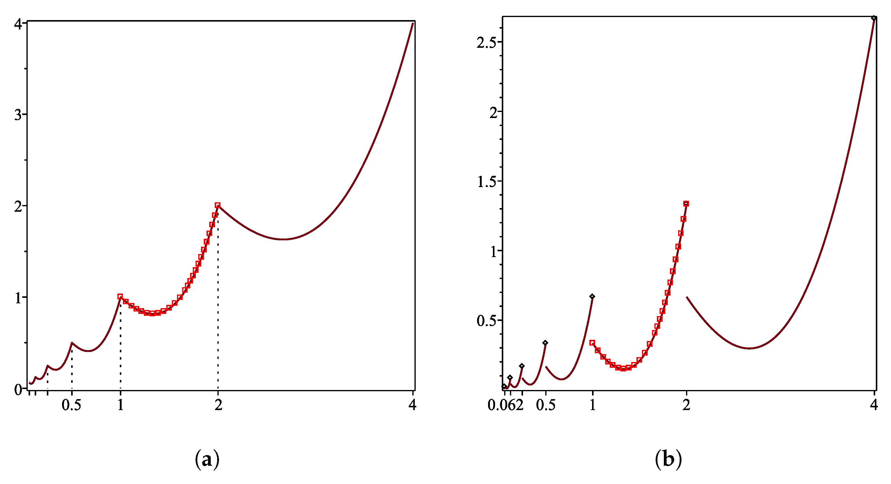
It is worth pointing out that the formulation of Equation (18) on the bounded interval ${\overline{I}}_0$ is correct and no initial functions are needed: all the operations with values of u that may appear in the right-hand side of (18) are well defined since the function is extended by symmetry. For example, if $\mu =1/2$, $\psi :t\mapsto 2t$, $J=[0,\infty )$, the operator f appearing in (1) has the form

$$\left(fu\right)\left(t\right)=u\left(\tau \right(t\left)\right),t\in J,$$

(27)

with a certain $\tau :J\to J$, and one needs to compute the values $\{\left(\tilde{f}v\right)\left(t\right):t\in [1,2]\}$ on the function $v\left(t\right)=t^2+2$, $t\in [1,2]$, then we substitute into (27) the corresponding function $v_{\ast }$ the graph of which is presented on Figure 2. We see, in particular, that $v_{\ast }$ is continuous because v satisfies (7). An easy computation shows that in this case,

$$\left(\tilde{f}v\right)\left(t\right)=\left\{\begin{array}{cc}{\left(\tau \left(t\right)\right)}^2+2\hfill & \mathrm{if}\tau \left(t\right)\in I_0,\hfill \\ 2^{-3k}{\left(\tau \left(t\right)\right)}^2+2^{1-k}\hfill & \mathrm{if}\tau \left(t\right)\in I_k,k=\pm 1,\pm 2,\cdots .\hfill \end{array}\right.$$

Lemma 4.

If ${f|}_{P{C}_{\sigma }\left(J\right)}$ is continuous as a mapping from $P{C}_{\sigma }\left(J\right)$ to $L_{\mathrm{loc}}\left(\tilde{J}\right)$, $\tilde{f}$ is continuous as a mapping from $C\left({\overline{I}}_0\right)$ to $L\left({\overline{I}}_0\right)$.

Proof. 

Let $\check{C}\left(J\right)=P{C}_{\sigma }\left(J\right)$ with $\sigma$ of form (13). Let $\{v_m:m\ge 1\}\subset C\left({\overline{I}}_0\right)$ and $v_m\to v$, $m\to \infty$, in $C\left({\overline{I}}_0\right)$. Construct the functions $v_{\ast }:J\to \mathbb{R}$ and $v_{m\ast }:J\to \mathbb{R}$, $m\ge 1$, according to (14). If $t\in I_{-1}$, then by (15), $\psi \left(t\right)\in I_0$ and (14) yields

$$|v_{m\ast }\left(t\right)-v_{\ast }\left(t\right)|=|\mu ||v_m\left(\psi \left(t\right)\right)-v_m\left(\psi \left(t\right)\right)|\le |\mu |\underset{s\in {\overline{I}}_0}{max}|v_m\left(s\right)-v\left(s\right)|$$

for all $t\in I_{-1}$ and $m\ge 1$. Similarly, for $t\in I_1$, we have ${\psi }^{-1}\left(t\right)\in I_0$, and by (14),

$$|v_{m\ast }\left(t\right)-v_{\ast }{\left(t\right)|=|\mu |}^{-1}|v_m\left({\psi }^{-1}\left(t\right)\right)-v_m\left({\psi }^{-1}\left(t\right)\right){|\le |\mu |}^{-1}\underset{s\in {\overline{I}}_0}{max}|v_m\left(s\right)-v\left(s\right)|$$

for all $t\in I_1$, $m\ge 1$. Continuing by analogy, we find that

$$\underset{t\in I_j}{sup}|v_{m\ast }\left(t\right)-v_{\ast }{\left(t\right)|\le |\mu |}^j\underset{t\in {\overline{I}}_0}{max}|v_m\left(t\right)-v\left(t\right)|$$

(28)

for all $j\in \mathbb{Z}$ and $m\ge 1$. Therefore,

$$\begin{array}{cc}\hfill \underset{-k\le j\le k}{max}\underset{t\in {({\psi \left(t_0\right)}^j,\psi \left(t_0\right))}^{j+1}}{sup}|v_{m\ast }\left(t\right)-v_{\ast }\left(t\right)|& \le \underset{-k\le j\le k}{max}{|\mu |}^j\underset{t\in {\overline{I}}_0}{max}|v_m\left(t\right)-v\left(t\right)|\hfill \\ \hfill & ={|\mu |}^{k\mathrm{sign}(|\mu |-1)}\underset{t\in {\overline{I}}_0}{max}|v_m\left(t\right)-v\left(t\right)|\to 0\hfill \end{array}$$

(29)

as $m\to \infty$ for every $k\ge 1$, i.e., ${lim}_{m\to \infty }{v}_{m\ast }=v_{\ast }$ in $P{C}_{\sigma }\left(J\right)$. The continuity of $f:P{C}_{\sigma }\left(J\right)\to L_{\mathrm{loc}}\left(\tilde{J}\right)$ and definition (17) imply that $\tilde{f}\left(v_m\right)=f\left(v_{m\ast }\right)\to f\left(v_{\ast }\right)=\tilde{f}\left(v\right)$, $m\to \infty ,$ in $L_{\mathrm{loc}}\left(\tilde{J}\right)$. Since $\tilde{J}$ is an open neighborhood of the interval J, it follows that $\tilde{f}\left(v\right)$ has no non-integrable singularities on ${\overline{I}}_0$, and hence $\tilde{f}\left(v\right)\in C\left({\overline{I}}_0\right)$.

If $\check{C}\left(J\right)=L_{\mathrm{loc}}^{\infty }\left(J\right)$ and $\{v,v_1,v_2,\cdots \}\subset C\left({\overline{I}}_0\right)$ are as above, then ${\mathrm{ess}\sup }_{t\in I_k}|v_{m\ast }\left(t\right)-v_{\ast }\left(t\right)|$ can be estimated using (29), and the same argument can be applied. □

Lemmata 1 and 3 allow us to replace the problem of finding a solution $u:J\to \mathbb{R}$ of (1) with property (2) by the two-point problem (7) and (18) on the bounded interval ${\overline{I}}_0$. Lemma 4 ensures that we are under standard assumptions concerning boundary value problems for first-order functional differential equations.

The above-mentioned facts are true in particular for the operators involving inner superpositions, which may have the form

$$\left(fu\right)\left(t\right)=h(t,u\left({\tau }_1\left(t\right)\right),\cdots ,u\left({\tau }_m\left(t\right)\right)),t\in J,$$

(30)

where $h:J\to \mathbb{R}$ is a Carathéodory function and ${\tau }_i:J\to J$, $i=1,2,\cdots ,m$, are measurable. In this case, (1) is an equation with argument deviations, and the procedure of restriction of Equation (1) to the bounded interval ${\overline{I}}_0$, in fact, corresponds to the well-known techniques from [5]. The symmetry condition (3) for operator (30) can be verified, e.g., using the following simple lemma.

Lemma 5.

Let there exist integers $k_1$, $k_2$, ⋯, $k_m$ such that

$${\tau }_i\circ \psi ={\psi }^{k_i}\circ {\tau }_i,i=1,2,\cdots ,m,$$

(31)

and

$${\psi }^{\prime }\left(t\right)h(\psi \left(t\right),{\mu }^{-k_1}{z}_1,{\mu }^{-k_2}{z}_2,\cdots ,{\mu }^{-k_m}{z}_m)={\mu }^{-1}h(t,z_1,z_2,\cdots ,z_m)$$

(32)

for all real $z_1$, ⋯, $z_m$ and almost every $t\in J$. Then the operator $f:\check{C}\left(J\right)\to L_{\mathrm{loc}}\left(J\right)$ given by (30) satisfies condition (3).

Proof. 

The proof is based on assumption (31). Indeed, let $u\in C\left(J\right)$ be such that (2) holds. Then $u\left(\psi \left(t\right)\right)={\mu }^{-1}u\left(t\right)$, $t\in J$, and (31) yields

$$u\left({\psi }^{k_i}\left({\tau }_i\left(t\right)\right)\right)={\mu }^{-1}u\left({\psi }^{k_i-1}\left({\tau }_i\left(t\right)\right)\right)=\cdots ={\mu }^{-k_i}u\left({\tau }_i\left(t\right)\right),t\in J,i=1,2,\cdots ,m.$$

By virtue of (32),

$$\mu {\psi }^{\prime }\left(t\right)h(\psi \left(t\right),{\mu }^{-k_1}u\left({\tau }_1\left(t\right)\right),\cdots ,{\mu }^{-k_m}u\left({\tau }_m\left(t\right)\right))=h(t,u\left({\tau }_1\left(t\right)\right),\cdots ,u\left({\tau }_m\left(t\right)\right)),$$

which in view of the arbitrariness of u with property (2), proves (3). □

Lemma 5 allows us to check condition (3) for a class of equations with argument deviations and carry out the transition from (1) and (2) to (7) and (18). For example, consider the problem

$$\begin{array}{cc}\hfill u^{\prime }\left(t\right)& =b\left(t\right)+\frac{{\left(u\left({\tau }_1\left(t\right)\right)\right)}^{2\nu +1}}{a\left(t\right)+{\left(u\left({\tau }_2\left(t\right)\right)\right)}^{2\nu }},\hfill \end{array}$$

(33)

$$\begin{array}{cc}\hfill u\left(t\right)& =\mu u(t+\mu ),t\in (-\infty ,\infty ),\hfill \end{array}$$

(34)

where $\nu >0$ and $\mu >0$ are constants, a, b are functions integrable on every bounded interval, and such that a is positive,

$$\begin{array}{cc}\hfill a(t+\mu )& ={\mu }^{-2\nu }a\left(t\right),\hfill \end{array}$$

(35)

$$\begin{array}{cc}\hfill b(t+\mu )& ={\mu }^{-1}b\left(t\right)\hfill \end{array}$$

(36)

for all $t\in (-\infty ,\infty )$, and

$${\tau }_i\left(t\right):=n_{i}t+{\beta }_i,t\in (-\infty ,\infty ),i=1,2,$$

(37)

with $\{n_1,n_2\}\subset \mathbb{Z}$ and $\{{\beta }_1$, ${\beta }_2\}\subset \mathbb{R}$.

Define f by (30) with $m=2$, $h:(t,z_1,z_2)\mapsto b\left(t\right)+z_1^{2\nu +1}/(a\left(t\right)+z_2^{2\nu }).$ Then problem (33) and (34) is a particular case of (1) and (2) with $\psi :t\to t+\mu$ on $J=(-\infty ,\infty )$ (it is obvious that ${\alpha }^{-}=-\infty$ and ${\alpha }^{+}=\infty$ in (10) for this case). It is easy to see that functions (37) satisfy condition (31), which means here that

$${\tau }_i(t+\mu )={\tau }_i\left(t\right)+n_i\mu ,t\in (-\infty ,\infty ),$$

where $n_1$, $n_2$ are integers. Furthermore, by (35) and (36),

$$\begin{array}{cc}\hfill \mu h(t+\mu ,{\mu }^{-1}{z}_1,{\mu }^{-1}{z}_2)& =\mu b(t+\mu )+\mu \frac{z_1^{2\nu +1}{\mu }^{-2\nu -1}}{a(t+\mu )+z_2^{2\nu }{\mu }^{-2\nu }}\hfill \\ \hfill & =b\left(t\right)+\mu \frac{z_1^{2\nu +1}{\mu }^{-2\nu -1}}{{\mu }^{-2\nu }a\left(t\right)+z_2^{2\nu }{\mu }^{-2\nu }}=h(t,z_1,z_2)\hfill \end{array}$$

for any t and $z_1$, $z_2$, i.e., h satisfies condition (32) with the given $\psi$ and $k_1=1$, $k_2=1$. Consequently, the problem of finding solutions $u:\mathbb{R}\to \mathbb{R}$ of (33) possessing property (34) can be replaced by the corresponding two-point problem (7) and (18) on a bounded interval of length $\mu$.

4. Existence of a Unique Symmetric Solution

We formulate conditions in terms of the “restriction” operator $\tilde{f}$ given by (17). Consider the case where the operator $\tilde{f}$ admits the estimate

$$|\left(\tilde{f}u\right)\left(t\right)-\left(\tilde{f}v\right)\left(t\right)+g_1(u-v)\left(t\right)|\le g_0(u-v)\left(t\right),t\in {\overline{I}}_0,$$

(38)

for all $u,v$ from $C\left({\overline{I}}_0\right)$, where $g_i:C\left({\overline{I}}_0\right)\to L\left({\overline{I}}_0\right)$, $i=0,1$, are certain positive linear operators. By a positive operator, we mean an operator $p:C\left({\overline{I}}_0\right)\to L\left({\overline{I}}_0\right)$ such that ${\mathrm{ess}\inf }_{t\in {\overline{I}}_0}\left(pu\right)\left(t\right)\ge 0$ for all $u\in C\left({\overline{I}}_0\right)$ such that ${min}_{t\in {\overline{I}}_0}u\left(t\right)\ge 0$.

Theorem 1.

Let there exist positive linear operators $g_i:C\left({\overline{I}}_0\right)\to L\left({\overline{I}}_0\right)$, $i=0,1$, such that (38) holds for all $u,v$ from $C\left({\overline{I}}_0\right)$. Let $|\mu |\le 1$ and

$$\frac{1-|\mu |}{|\mu |}<\theta \parallel g_1\left(1\right)\parallel \le |\mu |$$

(39)

with a certain $\theta \in (0,1)$. In addition, assume that

$$\parallel g_0\left(1\right)\parallel +(1-2\theta )\parallel g_1\left(1\right)\parallel <1-|\mu |$$

(40)

if $0<\theta \le 1/2$ or

$$\begin{array}{cccc}\hfill \parallel g_0\left(1\right)\parallel & <1,\hfill & \hfill \frac{\parallel g_0\left(1\right)\parallel }{1-\parallel g_0\left(1\right)\parallel }-\frac{1-|\mu |}{|\mu |}& <(2\theta -1)\parallel g_1\left(1\right)\parallel \le |\mu |\hfill \end{array}$$

(41)

if $1/2<\theta <1$. Then Equation (1) has a unique solution possessing property (2).

In (39)–(41) and similar relations below, $g_i\left(1\right)$ stands for the value of $g_i$ on the constant function equal to 1, and $∥·∥$ is the norm in $L\left({\overline{I}}_0\right)$.

Theorem 2.

Let there exist positive linear operators $g_i:C\left({\overline{I}}_0\right)\to L\left({\overline{I}}_0\right)$, $i=0,1$, such that (38) holds for all $u,v$ from $C\left({\overline{I}}_0\right)$. Let $|\mu |\ge 1$ and

$$|\mu |-1<\theta \parallel g_1\left(1\right)\parallel \le 1$$

(42)

with some $\theta \in (0,1)$. In addition, assume that

$$\parallel g_0\left(1\right)+(1-2\theta )g_1\left(1\right)\parallel <\frac{1}{|\mu |}$$

(43)

if $0<\theta \le 1/2$ or

$$\begin{array}{cccc}\hfill \parallel g_0\left(1\right)\parallel & <\frac{1}{|\mu |},\hfill & \hfill \frac{|\mu |}{1-|\mu |\parallel g_0\left(1\right)\parallel }-1& <(2\theta -1)\parallel g_1\left(1\right)\parallel \le 1\hfill \end{array}$$

(44)

if $1/2<\theta <1$. Then Equation (1) has a unique solution possessing property (2).

Condition (38) is satisfied, in particular, if (1) is a linear equation of the form

$$u^{\prime }\left(t\right)=\left(p_{0}u\right)\left(t\right)-\left(p_{1}u\right)\left(t\right)+r\left(t\right),t\in J,$$

(45)

where $p_i:\check{C}\left(J\right)\to L_{\mathrm{loc}}\left(\tilde{J}\right)$, $i=0,1$, are positive linear operators such that their restrictions to $C\left(J\right)$ are continuous mappings from $C\left(J\right)$ to $L_{\mathrm{loc}}\left(\tilde{J}\right)$ with some $\tilde{J}$ strictly containing J. In this case, the symmetry condition holds if $r\in L_{\mathrm{loc}}\left(\tilde{J}\right)$ is such that

$$\mu {\psi }^{\prime }\left(t\right)r\left(\psi \left(t\right)\right)=r\left(t\right),t\in J,$$

(46)

and

$$\mu {\psi }^{\prime }\left(t\right)\left(p_{i}u\right)\left(\psi \left(t\right)\right)=\left(p_{i}u\right)\left(t\right),t\in J,i=0,1,$$

(47)

for any absolutely continuous function u possessing property (2), and Theorems 1 and 2 can be applied (in fact, $p_0={\tilde{g}}_0$ and $p_1={\tilde{g}}_1$ in this case). Other conditions for the existence of symmetric solutions of (45) are given by the next two statements.

Theorem 3.

Assume (47). If $|\mu |\le 1$ and

$$\begin{array}{c}\parallel {\tilde{p}}_0\left(1\right)\parallel <2,\end{array}$$

(48)

$$\begin{array}{c}\frac{\parallel {\tilde{p}}_0\left(1\right)\parallel }{2-\parallel {\tilde{p}}_0\left(1\right)\parallel }-\frac{1-|\mu |}{|\mu |}<\frac{1}{2}\parallel {\tilde{p}}_1\left(1\right)\parallel \le |\mu |,\end{array}$$

(49)

then Equation (45) has a unique solution possessing property (2).

In (48) and (49) and relations (50) and (51) below, ${\tilde{p}}_i:C\left({\overline{I}}_0\right)\to L\left({\overline{I}}_0\right)$, $i=0,1$, are bounded linear operators constructed according to (17), and $∥·∥$ denotes the norm in $L\left({\overline{I}}_0\right)$.

Theorem 4.

Assume (47). If $|\mu |\ge 1$ and

$$\begin{array}{c}\parallel {\tilde{p}}_0\left(1\right)\parallel <\frac{2}{|\mu |},\end{array}$$

(50)

$$\begin{array}{c}\frac{2|\mu |}{2-|\mu |\parallel {\tilde{p}}_0\left(1\right)\parallel }-1<\frac{1}{2}\parallel {\tilde{p}}_1\left(1\right)\parallel \le 1,\end{array}$$

(51)

then Equation (45) has a unique solution possessing property (2).

Although all the conditions involve the “tilde” versions of the operators, they are verified, due to the symmetry, essentially in the same way as if the operators were given on $C\left(\right[a,b\left]\right)$ with $-\infty <a<b<\infty$. In particular, if (45) is the equation with two measurable argument deviations ${\tau }_i:J_c\to J_c$, $i=0,1$, with $J_c=[c,\infty )$, $c\in \mathbb{R}$,

$$u^{\prime }\left(t\right)=a_0\left(t\right)u\left({\tau }_0\left(t\right)\right)-a_1\left(t\right)u\left({\tau }_1\left(t\right)\right)+r\left(t\right),t\in J_c,$$

(52)

then by Lemma 5, conditions (47) hold when there exist integers $k_0$, $k_1$ such that

$${\tau }_i\circ \psi ={\psi }^{k_i}\circ {\tau }_i,i=0,1,$$

(53)

the function $r\in L_{\mathrm{loc}}\left(J_{c-ϵ}\right)$ ($ϵ>0$) satisfies (46), and the functions $a_i\in L_{\mathrm{loc}}\left(J_{c-ϵ}\right)$, $i=0,1$ are such that

$${\psi }^{\prime }\left(t\right)a_i\left(\psi \left(t\right)\right)={\mu }^{k_i-1}{a}_i\left(t\right),t\in J_c,i=0,1.$$

(54)

Let us choose $t_0$ and c so that $t_0\ge c$ and ${lim}_{k\to \infty }{\psi }^{-k}\left(t_0\right)=c$, ${lim}_{k\to \infty }{\psi }^k\left(t_0\right)=\infty$ (e.g., if $\psi :t\mapsto \alpha t$, where $\alpha >1$, then $c=0$ with any $t_0>0$). By virtue of Theorems 3 and 4, if $a_i\ge 0$, $i=0,1$ and assumptions (46), (53) and (54) hold, then Equation (52) has a unique solution with property (2) provided that the integrals of $a_0$, $a_1$ over $[t_0,\psi \left(t_0\right)]$ lie within the bounds

$$\begin{array}{cccc}\hfill {\int }_{t_0}^{\psi \left(t_0\right)}{a}_0\left(t\right)dt& <2,\hfill & \hfill \hspace{1em}\hspace{1em}\hspace{1em}\hspace{1em}\frac{{\int }_{t_0}^{\psi \left(t_0\right)}{a}_0\left(t\right)dt}{2-{\int }_{t_0}^{\psi \left(t_0\right)}{a}_0\left(t\right)dt}-\frac{1-|\mu |}{|\mu |}& <\frac{1}{2}{\int }_{t_0}^{\psi \left(t_0\right)}{a}_1\left(t\right)dt\le |\mu |\hfill \end{array}$$

if $|\mu |\le 1$ and

$$\begin{array}{ccc}\hfill {\int }_{t_0}^{\psi \left(t_0\right)}{a}_0\left(t\right)dt& <\frac{2}{|\mu |},\hfill & \hfill \hspace{1em}\hspace{1em}\hspace{1em}\hspace{1em}\frac{2|\mu |}{2-|\mu |{\int }_{t_0}^{\psi \left(t_0\right)}{a}_1\left(t\right)dt}-1<\frac{1}{2}{\int }_{t_0}^{\psi \left(t_0\right)}{a}_1\left(t\right)dt\le 1\end{array}$$

if $|\mu |>1$. For example, when $\psi :t\mapsto \alpha t$ ($\alpha >1$), conditions (54) are satisfied if $1\notin \{k_0,k_1\}$, $\mu >1$, and $a_i:t\mapsto c_i{t}^{m_i}$, $m_i=(k_i-1)\frac{ln\mu }{ln\alpha }-1$, $c_i\ge 0$, $i=0,1$.

5. Proofs

We need auxiliary propositions based on the results of [8,12,13]. Consider the two-point boundary value problem

$$\begin{array}{cc}\hfill v^{\prime }\left(t\right)& =\left(\tilde{f}v\right)\left(t\right),t\in {\overline{I}}_0,\hfill \end{array}$$

(55)

$$\begin{array}{cc}\hfill v\left(t_0\right)& =\mu v\left(\psi \left(t_0\right)\right),\hfill \end{array}$$

(56)

where $\tilde{f}$ is defined according to (17) and ${\overline{I}}_0$ is as in (11) and (12).

A solution of Equation (55) is defined as an absolutely continuous function satisfying (55) almost everywhere on ${\overline{I}}_0$.

Fix the value of $t_0$, and let the set $\mathcal{S}$ be defined as follows: $p\in \mathcal{S}$ if and only if $p:C\left({\overline{I}}_0\right)\to L\left({\overline{I}}_0\right)$ is a bounded linear operator such that the equation

$$\begin{array}{c}{v}^{\prime }\left(t\right)=\left(pv\right)\left(t\right)+q\left(t\right),t\in {\overline{I}}_0,\end{array}$$

(57)

$$\begin{array}{c}v\left(t_0\right)=\mu v\left(\psi \left(t_0\right)\right)\end{array}$$

(58)

has a unique solution v in $C\left({\overline{I}}_0\right)$ for any $q\in L\left({\overline{I}}_0\right)$, and ${min}_{t\in {\overline{I}}_0}v\left(t\right)\ge 0$ whenever ${\mathrm{ess}\inf }_{t\in {\overline{I}}_0}q\left(t\right)\ge 0$.

Proposition 1

([12]). Let there exist positive linear operators $g_i:C\left({\overline{I}}_0\right)\to L\left({\overline{I}}_0\right)$, $i=0,1$, such that (38) holds for all $u,v$ from $C\left({\overline{I}}_0\right)$. If, in addition, the inclusions

$$\begin{array}{cccc}\hfill g_0+(1-2\theta )g_1& \in \mathcal{S},\hfill & \hfill \hspace{1em}\hspace{1em}\hspace{1em}\hspace{1em}-\theta g_1& \in \mathcal{S}\hfill \end{array}$$

(59)

hold with some constant $\theta \in (0,1)$, then problem (55) and (56) is uniquely solvable.

Proposition 2

([13]). Assume that $p:C\left({\overline{I}}_0\right)\to L\left({\overline{I}}_0\right)$ is a linear operator of the form

$$p=p_0-p_1,$$

(60)

where $p_i:C\left({\overline{I}}_0\right)\to L\left({\overline{I}}_0\right)$, $i=0,1$, are positive linear operators such that

$$\begin{array}{cccc}\hfill p_0& \in \mathcal{S},\hfill & \hfill \hspace{1em}\hspace{1em}\hspace{1em}\hspace{1em}\frac{1}{2}(p_0-p_1)& \in \mathcal{S}.\hfill \end{array}$$

(61)

Then problem (57) and (58) is uniquely solvable for any $q\in L\left({\overline{I}}_0\right)$.

We also need the following statements that are obtained from results of the work [8].

Proposition 3.

Let $g_i:C\left({\overline{I}}_0\right)\to L\left({\overline{I}}_0\right)$, $i=0,1$, be positive linear operators. Let $|\mu |\le 1$ and (39) holds with some $\theta \in (0,1)$. In addition, assume (40) if $0<\theta \le 1/2$ or (41) in the case where $1/2<\theta <1$. Then inclusions (59) hold.

Proposition 4.

Let $g_i:C\left({\overline{I}}_0\right)\to L\left({\overline{I}}_0\right)$, $i=0,1$, be positive linear operators. Let $|\mu |\ge 1$ and (42) holds with some $\theta \in (0,1)$. In addition, assume (43) if $0<\theta \le 1/2$ or (44) if $1/2<\theta <1$. Then inclusions (59) hold.

Propositions 3 and 4 are consequences of Theorems 2.4 and 2.8 from [8], which provide conditions guaranteeing the positivity of the corresponding Green’s operator for the two-point problem

$$\begin{array}{c}{u}^{\prime }\left(t\right)=\left(l_{0}u\right)\left(t\right)-\left(l_{1}u\right)\left(t\right)+q\left(t\right),t\in [a,b],\end{array}$$

(62)

$$\begin{array}{c}\lambda u\left(a\right)+\mu u\left(b\right)=c,\end{array}$$

(63)

with $q\in L\left(\right[a,b\left]\right)$, positive $l_i:C\left([a,b]\right)\to L\left([a,b]\right)$, $i=0,1$, and $-\infty <a<b<\infty$. In our case, the set $\mathcal{S}$ corresponds to $V_{t_0,\psi \left(t_0\right)}^{+}(1,\mu )$ from [8].

Let $|\mu |\le 1$. Then, according to [8] (Theorem 2.4), $l_0-l_1\in \mathcal{S}$ provided that $\parallel l_0\left(1\right)\parallel <1$ and $\parallel l_0\left(1\right)\parallel /(1-\parallel l_0\left(1\right)\parallel )-{|\mu |}^{-1}(1-|\mu |)<\parallel l_1\left(1\right)\parallel \le |\mu |$. The first operator in (59) is positive if $\theta \in (0,1/2]$, and the above formulae with zero $l_1$ yield $\parallel g_0\left(1\right)+(1-2\theta )g_1\left(1\right)\parallel <1$ and

$$\frac{\parallel g_0\left(1\right)+(1-2\theta )g_1\left(1\right)\parallel }{1-\parallel g_0\left(1\right)+(1-2\theta )g_1\left(1\right)\parallel }<\frac{1-|\mu |}{|\mu |},$$

which means that $\parallel g_0\left(1\right)+(1-2\theta )g_1\left(1\right)\parallel <1-|\mu |$. Since the norm in $L\left({\overline{I}}_0\right)$ is additive on non-negative functions, we get (43). For $\theta \in (1/2,1)$, representing the first mapping from (59) in the form $g_0+(1-2\theta )g_1=g_0-|1-2\theta |g_1,$ we apply the formulae mentioned with $l_0=g_0$, $l_1=|1-2\theta |g_1$, and get (44). Finally, condition (42) follows from the above inequalities with $l_0=0$, $l_1=\theta g_1$ and ensures the second inclusion in (59). Proposition 4 is obtained from [8] (Theorem 2.8) in a similar way.

In order to prove Theorem 1, we note that the assumptions made on f (and the continuity of $g_0$ and $g_1$ from condition (38) guarantee that $\tilde{f}:C\left({\overline{I}}_0\right)\to L\left({\overline{I}}_0\right)$ is continuous. It is sufficient to establish the solvability of the two-point problem (55) and (56). Let $|\mu |\le 1$. By Proposition 1 and (55) and (56) is solvable if one can specify some $\theta$, $0<\theta <1$, such that $g_0$ and $g_1$ from (38) satisfy conditions (59). According to Proposition 3, their fulfillment is a consequence of assumptions (40) and (42). The case $|\mu |\ge 1$ is treated similarly using Propositions 1 and 4.

Theorems 3 and 4 are obtained from the following statement.

Proposition 5.

Let $p_i:C\left({\overline{I}}_0\right)\to L\left({\overline{I}}_0\right)$, $i=0,1$, be positive linear operators. Assume that either $|\mu |\le 1$ and (48) and (49) hold or $|\mu |\ge 1$ and (50) and (51) hold. Then inclusions (61) are true.

Proposition 5 is proved by applying the above-mentioned Theorems 2.4 and 2.8 of [8] to the operator $(1/2){\tilde{p}}_0-(1/2){\tilde{p}}_1$ on $C\left([t_0,\psi \left(t_0\right)]\right)$. Note that under our assumptions, ${\tilde{p}}_0$ and ${\tilde{p}}_1$ constructed according to (17) are bounded linear operators acting from $C\left({\overline{I}}_0\right)$ to $L\left({\overline{I}}_0\right)$. When the validity of (61) is established, the assertions of Theorems 3 and 4 follow from Proposition 2.