Article

Numerical Method for Dirichlet Problem with Degeneration of the Solution on the Entire Boundary

by
Viktor A. Rukavishnikov
*,† and
Elena I. Rukavishnikova
Computing Center of Far-Eastern Branch, Russian Academy of Sciences, Kim-Yu-Chen Str. 65, Khabarovsk 680000, Russia
*
Author to whom correspondence should be addressed.
These authors contributed equally to this work.
Symmetry 2019, 11(12), 1455; https://doi.org/10.3390/sym11121455
Submission received: 10 November 2019 / Revised: 22 November 2019 / Accepted: 23 November 2019 / Published: 26 November 2019
(This article belongs to the Special Issue Mesh Methods - Numerical Analysis and Experiments)

Abstract

:
The finite element method (FEM) with a special graded mesh is constructed for the Dirichlet boundary value problem with degeneration of the solution on the entire boundary of the two-dimensional domain. A comparative numerical analysis is performed for the proposed method and the classical finite element method for a set of model problems in symmetric domain. Experimental confirmation of theoretical estimates of accuracy is obtained and conclusions are made.

1. Introduction

As is known, classical solutions for boundary value problems for elliptic equations with discontinuous coefficients do not exist. Therefore, the notion of a generalized (weak) solution was introduced. Based on this definition and on the Galerkin method, numerous numerical methods were developed for finding approximate solutions of such problems. However, these methods for boundary value problems with singularity lose accuracy, which depends on the smoothness of the solution of the original differential problem (see, for example, [1,2]). The singularity of the solution of the boundary value problem can be caused by the presence of re-entrant corners on the domain boundary, by the degeneration of the coefficients and right-hand sides of equation and boundary conditions, or by the internal properties of the solution (see, for example, [3,4,5,6,7,8,9]). For boundary problems with a singularity, we proposed to determine an R ν -generalized solution. The existence, uniqueness and differential properties of this kind of solution in the weighted Sobolev spaces were studied in [10,11,12,13,14,15]. Based the R ν -generalized solution, a weighted finite element method was developed for boundary value problems for elliptic equations in two-dimensional domain with a singularity in a finite set of boundary points [16,17,18,19,20]. A weighted FEM was constructed and studied for the Lamé system in a domain with re-entrant corners [21,22]. To find an approximate solution of Maxwell’s equations in an L-shaped domain, a weighted edge-based finite element method was proposed in [23,24]. In [25,26] a weight analogue of the condition of Ladyzhenskaya-Babuška-Brezzi was proved, a numerical method was developed for the Stokes and Oseen problems in domains with corner singularity. The main feature of all the developed methods is the convergence of the approximate solution to the exact one with the rate O ( h ) in the norms of the Sobolev and Monk weighted spaces, regardless of the reasons causing the solution singularity and its value.
In this paper we consider the Dirichlet problem for an elliptic equation with degeneration of the solution on the entire boundary of a two-dimensional domain. In [27] a finite element method was constructed for this problem and the convergence of this method was established. The paper [28] singles out the weighted subspace of functions for which the approximate solutions converge to an exact solution with a speed O ( h ) on a mesh with a special compression of nodes close to the boundary (see [29]). The compression parameters depend on the constructed subspace. Our method of constructing mesh with a special compression of nodes differs from the methods proposed by other authors (see, for example, [30,31,32]).
Here we test model problems with singularities in a symmetric domain. We carry out a comparative numerical analysis of finite element methods on quasi-uniform meshes and meshes with a special compression of nodes close to the boundary. We obtain experimental confirmation of theoretical estimates and demonstrate the advantage of the proposed method over the classical finite element method. By analogy with [22], we found that it is impossible to use FEM with a strong thickening of mesh, and introduction of an R-generalized solution is required. The existence and uniqueness of the R-generalized solution for this problem were proved in [33].

2. Problem Formulation

Let Ω be a bounded convex two-dimensional domain with twice differentiable boundary Ω , and let Ω ¯ be the closure of Ω , i.e., Ω ¯ = Ω Ω ; x = ( x 1 , x 2 ) and d x = d x 1 d x 2 .
We assume that a positive function ρ ( x ) belongs to the space C ( 2 ) ( Ω ) and coincides in the boundary strip of width d > 0 with the distance from x ( x Ω ) to the boundary Ω .
We introduce the weighted Sobolev space W 2 , η s ( Ω ) with the norm
v W 2 , η s ( Ω ) = v L 2 ( Ω ) + | m | = s m 1 , m 2 = 0 ρ η | m | v x 1 m 1 x 2 m 2 L 2 ( Ω ) ,
where η is a real number satisfying the inequalities 1 2 s < η < 1 2 ; s = 1 , 2 ; m = ( m 1 , m 2 ) , | m | = m 1 + m 2 , m 1 , m 2 are integer nonnegative numbers.
Let
W ˚ 2 , η s ( Ω ) = { v : v W 2 , η s ( Ω ) , v | Ω = 0 } .
We denote by L 2 , 1 η ( Ω ) the space of functions f with the norm
f L 2 , 1 η ( Ω ) = Ω | ρ 1 + η f | 2 d x 1 / 2 .
We consider the first boundary value problem for a second order elliptic equation
k = 1 2 x k a k k ( x ) u x k + a ( x ) u = f in Ω , u = 0 on Ω .
We suppose that the input data of Equation (1) satisfy the conditions:
(a)
f L 2 , 1 α ( Ω ) ,
(b)
a k k ( x ) ( k = 1 , 2 ) are differentiable functions on Ω , such that the inequalities
| a k k ( x ) | C 1 ρ 2 α ( x ) ,
| a k k ( x ) x 1 | , | a k k ( x ) x 2 | C 2 ρ 2 α 1 ( x ) ,
k = 1 2 a k k ( x ) ξ k 2 C 3 ρ 2 α ( x ) k = 1 2 ξ k 2 , x Ω , C 3 > 0 ,
hold,
(c)
the function a ( x ) satisfies the inequalities
0 < a ( x ) C 4 ρ 2 α 2 ( x ) , x Ω .
Here C i , ( i = 1 , , 4 ) are constants independent of x, ξ 1 and ξ 2 are any real parameters, α 1 2 , 1 2 .
Remark 1.
If Conditions (2)–(6) are fulfilled for the input data, Equation (1) is called a Dirichlet boundary value problem for an elliptic equation with degeneration of the solution on the entire boundary of a two-dimensional domain. Such problems are encountered in gas dynamics, electromagnetism and other subject areas of mathematical physics. The differential properties of solutions of problems with degeneracy on the entire boundary were studied, for the first time, in [7,8,9].
We introduce the bilinear and linear forms
E ( u , w ) = Ω k = 1 2 a k k ( x ) u x k w x k + a ( x ) u w d x , ( f , w ) = Ω f w d x .
A function u in W ˚ 2 , α 1 ( Ω ) is called a generalized solution of the first boundary value Equation (1) if for any w in W ˚ 2 , α 1 ( Ω ) the identity
E ( u , w ) = ( f , w )
holds.
We note that if Conditions (2)–(6) are satisfied, then there exists a unique generalized solution of the Equation (1) in the space W ˚ 2 , α 1 ( Ω ) (see Theorem 1 from [8]). In addition u W ˚ 2 , α 1 2 ( Ω ) (see Theorem 1 from [9]). Moreover, if the function f L 2 , 1 α + λ ( Ω ) L 2 , 1 α ( Ω ) 1 2 < α < α + λ < 1 2 and the parameter λ is sufficiently small, then the generalized solution u belongs to the space W ˚ 2 , α + λ 1 2 ( Ω ) which is a subspace of W ˚ 2 , α 1 2 ( Ω ) (see [28]).
Remark 2.
Knowing that the solution belongs to the space W ˚ 2 , α + λ 1 2 ( Ω ) allows us to construct a finite element method for finding a generalized solution for the Dirichlet problem with the degeneration of the solution on the entire boundary of the domain with a convergence speed O ( h ) in the norm W 2 , α 1 ( Ω ) .

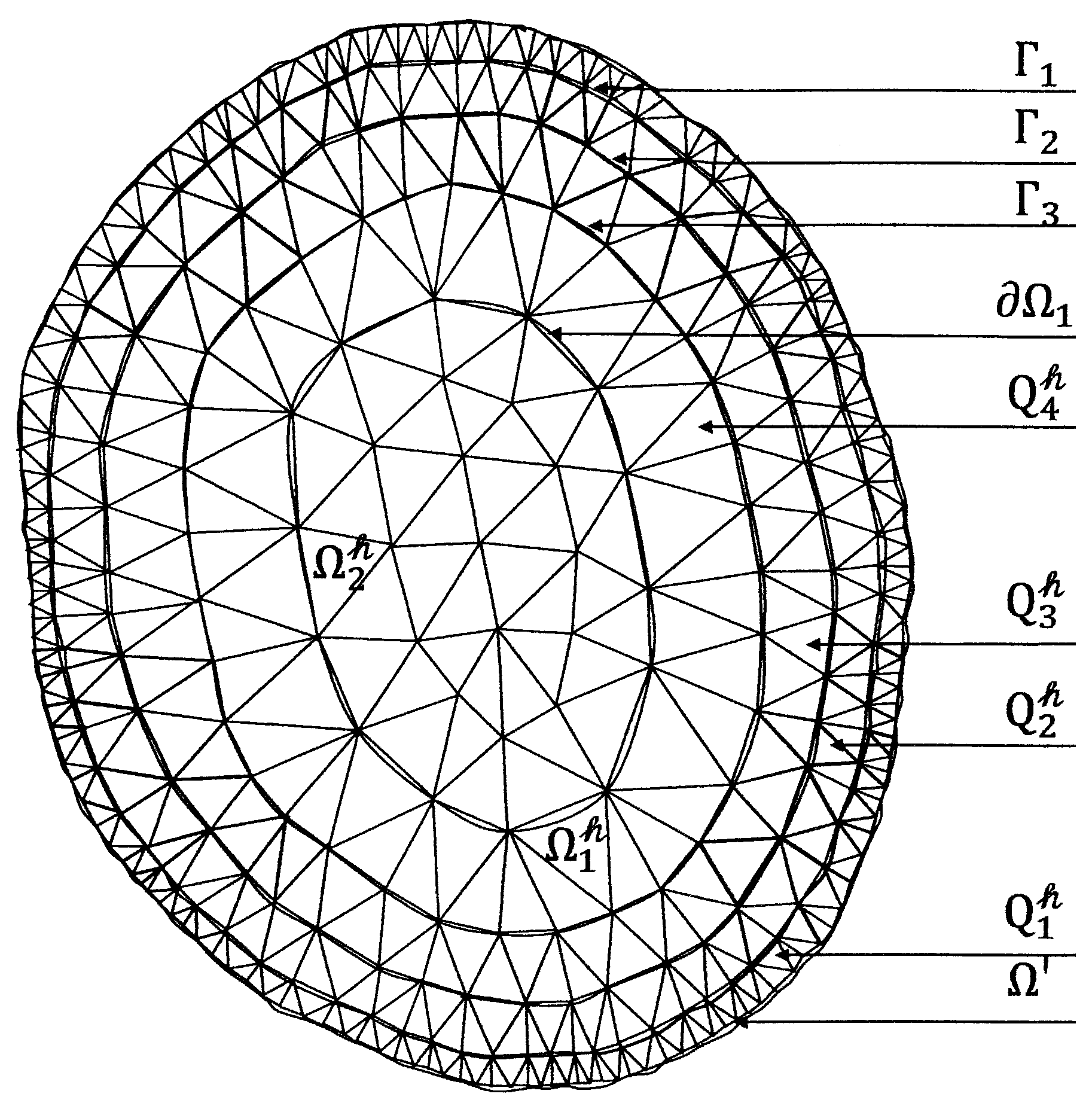
3. The Scheme of the Finite Element Method

We construct a scheme of the finite element method for finding an approximate generalized solution of the first boundary value Equation (1). We perform a triangulation of the domain Ω (see, for example, Figure 1).
We draw the curves Γ j , j = 0 , , n , at distance b j n r , j = 0 , , n , to the boundary Ω . Here r is the exponent of compression and r > 1 ; 0 < b < δ Ω 2 d , δ Ω is the diameter of the circle inscribed in Ω . In this case the line Γ n divides the domain Ω into two subdomains Ω 1 and Ω 2 . The subdomain Ω 1 is the outer domain on the boundary strip of width b, Ω 2 is the inner domain. On each curve Γ j , j = 0 , , n , ( Γ 0 = Ω , Γ n = Ω 1 ) we fix M j equidistant points, which we call the nodes. Here  M j = l j / b j n r j 1 n r + 1 , j = 1 , , n , l j is the length of the curve Γ j ( [ x ] denotes the integer part of x) and M 0 = 2 M 1 . All nodes on the curve Γ j , j = 0 , , n , are connected by the broken line. Then, we connect each node on the curve Γ j 1 , j = 1 , , n , with closest nodes on the curve Γ j . As a result, the subdomain Ω 1 is divided into triangles with the compression of nodes to the boundary Ω . The union of all triangles with vertices on Γ j 1 and Γ j is a layer Q j h . (In Figure 1 the subdomain Ω 1 is divided into the layers Q 1 h , , Q 4 h , Γ 4 = Ω 1 ). The parameter h denotes the greatest in length of the sides of the triangles in Q n h .
The subdomain Ω 2 is divided quasi-uniformly into a finite number of the triangles. The sides of these triangles can not be greater than h. Moreover, the vertices of the triangles on the boundary Ω 1 belong to the set of vertices of the triangles in Ω 2 .
The algorithm and code description of this triangulation are given in [29].
Let Ω h be the union of closed triangles { K } = { K 1 , , K N h } , and K j , j = 1 , , N h , is the finite element. The vertices G i , i = 1 , , N , of these triangles are the nodes of the triangulation. We denote by N the number of the internal nodes. To each node G i , i = 1 , , N , we assign the function φ i ( x ) which is equal to 1 at the point G i and zero at all other nodes, and φ i ( x ) is linear on each triangle K. We denote by V h the linear span { φ i } i = 1 N . Next, we associate the following discrete problem with the constructed finite-dimensional space V h W ˚ 2 , α 1 ( Ω ) : find the function u h V h satisfying the equality
E ( u h , w h ) = ( f , w h )
for any function w h V h .
An approximate (finite element) generalized solution will be found in the form
u h ( x ) = i = 1 N a i φ i ( x ) ,
where a i = u h ( G i ) . We assume that u h ( x ) = 0 , x Ω \ Ω h .
The coefficients a i are defined from system of equations
E ( u h , φ i ) = ( f , φ i ) , i = 1 , , N
or
A ^ a = F ,
where
a = ( a 1 , , a N ) T , F = ( F 1 , , F N ) T , A ^ = ( A i j ) ,
A i j = E ( φ i , φ j ) , F i = ( f , φ i ) , i , j = 1 , , N .
It is obvious that the approximate generalized solution of Problems (1)–(6) by the finite element method exists and is unique.
For the performed triangulation of the domain Ω with the exponent of the compression of the mesh r = 1 λ and for functions in the space W ˚ 2 , α + λ 1 2 ( Ω ) we have convergence estimates:
u u h W 2 , α 1 ( Ω ) C 5 h f ρ 1 + α λ L 2 ( Ω ) ,
u u h L 2 ( Ω ) C 6 h 2 f ρ 1 + α λ L 2 ( Ω ) .
Here, the positive constants C 5 , C 6 are independent of u, u h , f and h.

4. Numerical Experiments

In this section we present the results of numerical experiments for two model problems.
Let Ω be a circle of unit radius with center at the point ( 2 , 2 ) . We consider the boundary value Equation (1) in the domain Ω . The right-hand side and coefficients of Equation (1) are given as
f ( x ) = 4 ( 1 + μ t ) ( μ 2 α t ) ρ ˜ μ 2 α t 1 ( x ) ( 1 ρ ˜ ( x ) ) ρ ˜ μ 2 α t ( x ) + ρ ˜ 1 + μ t ( x ) ,
a 11 ( x ) = a 22 ( x ) = ρ ˜ 2 α ( x ) , a ( x ) = 1 , α 1 2 , 1 2 , μ α , 1 2 , t < 1 2 ,
where ρ ˜ ( x ) = 1 ( x 1 2 ) 2 ( x 2 2 ) 2 and ρ ˜ ( x ) be a function that is infinitely differentiable and satisfies the following conditions:
C 7 ρ ( x ) ρ ˜ ( x ) C 8 ρ ( x )   for each point   x   of the domain   Ω ; 0 < C 7 C 8 < .
The exact solution of this problem is u ( x ) = ρ ˜ 1 μ t ( x ) .
For finding an approximate solution of model problems we used mesh with the compression of nodes to the boundary ( R c ), quasi-uniform mesh ( R q ) and the finite element method scheme from paragraph three. For the mesh R c we set the number of layers n and the exponent of compression of the mesh r = 1 τ , τ = μ α .
We investigate the convergence rate of the approximate solution u h to the exact one in the norms of the spaces L 2 ( Ω ) and W 2 , α 1 ( Ω ) on the mesh R c and R q . The absolute value of the error e = | u u h | in the mesh nodes G i on the mesh R c and R q is analyzed.
Model Problem 1. We set the parameters α = 0.01 , μ = 0.49 , t = 0.499 , at which the solution, the coefficients and the right-hand side of the equation in Equation (1) have the form
u ( x ) = ρ ˜ 0.991 ( x ) ,
a 11 ( x ) = a 22 ( x ) = ρ ˜ 0.02 ( x ) , a ( x ) = 1 ,
f ( x ) = 0.114956 · ρ ˜ 1.029 ( x ) + 3.849044 · ρ ˜ 0.029 ( x ) + ρ ˜ 0.991 ( x ) ,
the exponent of compression of the mesh r = 2.08 ( 3 ) .
In Table 1 we give the number of nodes and their percentage to the total number of mesh nodes N, in which the absolute value of the error e = | u u h | is not less than the specified value of the limit error. In this Table the patterns of the absolute error distribution at the nodes of the R q and R c meshes are also showed. We present data on the R c mesh for N nodes and on the R q mesh for N and N 2 nodes.
In Table 2 we present the norms of the difference between an exact and an approximate solution e L 2 ( Ω ) = u u h L 2 ( Ω ) and e W 2 , α 1 ( Ω ) = u u h W 2 , α 1 ( Ω ) for R q and R c and find the ratios of the norms β when the mesh parameter h is reduced by a factor two. The value of the parameter h in the domain Ω 2 for R c varies by changing number of layers n.
The distribution of the absolute values of the error e in the mesh nodes with a decrease in the h parameter by a factor of two on the meshes R q and R c is given in Table 3.
Model Problem 2. We set the parameters α = 0.49 , μ = 0.01 , t = 0.49 , at which the solution, the coefficients and the right-hand side of Equation (1) have the form
u ( x ) = ρ ˜ 0.52 ( x ) ,
a 11 ( x ) = a 22 ( x ) = ρ ˜ 0.98 ( x ) , a ( x ) = 1 ,
f ( x ) = 1.04 · ρ ˜ 0.5 ( x ) + 3.12 · ρ ˜ 0.5 ( x ) + ρ ˜ 0.52 ( x ) ,
the exponent of compression of the mesh r = 2 .
A numerical analysis of this problem was carried out by analogy with Model Problem 1. The results of the research are presented in Table 4, Table 5 and Table 6.
In Figure 2a,b we present graphs of the error e W 2 , α 1 ( Ω ) = u u h W 2 , α 1 ( Ω ) as a function of the parameter h on the grids R q and R c in a logarithmic scale. In the first case the parameter h decreases due to an increase in the number of layers n at a fixed value b = 1 / 64 (Figure 2a). In the second case h changes due to a decrease in the width of the border strip b at a fixed number n (Figure 2b).

5. Conclusions

We can conclude according to the results of numerical experiments:
  • An approximate generalized solution of Equation (1) on grids with an appropriate compression of nodes (close) to the boundary of the domain converges to an exact solution with a speed O ( h 2 ) in the norm of the space L 2 ( Ω ) and O ( h ) in the norm of the space W 2 , α 1 ( Ω ) (see Table 2 and Table 5);
  • the absolute value of the error is an order of magnitude smaller on the mesh with the compression of nodes to the boundary of the domain and with an optimal choice of parameters b and n than on a quasi-uniform mesh (see Table 1, Table 3, Table 4 and Table 6);
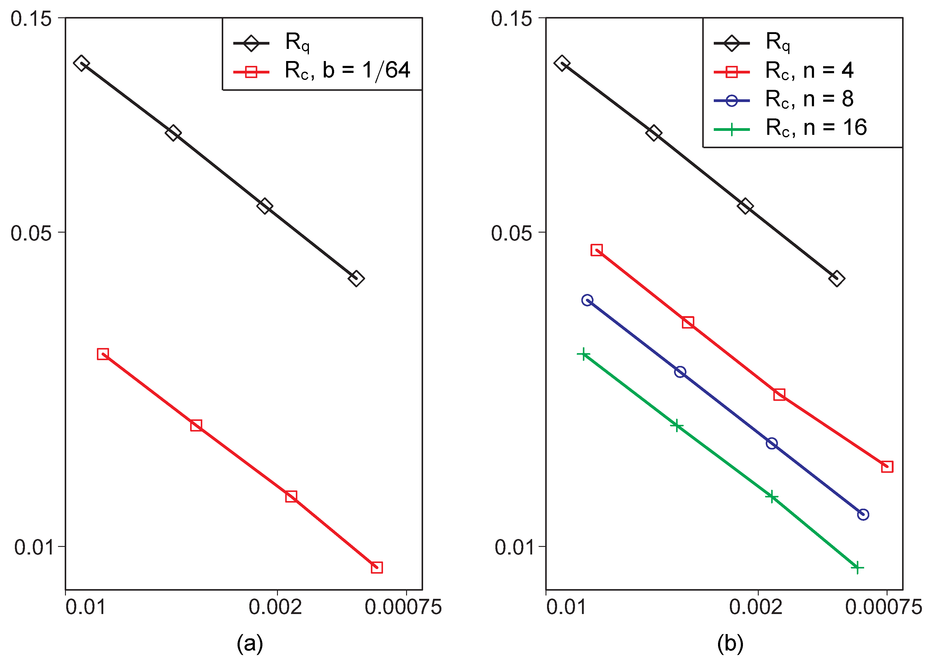
  • to reduce the absolute value of the error it is more expedient to increase the number of layers n than to reduce the width of the boundary ring domain; in this case the absolute value of the error decreases faster;
  • for meshes of large dimensionality it is advisable to use the weighted finite element method.
In the next papers we plan to develop the proposed finite element method for boundary value problems with inhomogeneous boundary conditions for self-adjoint differential equations of second and higher orders with weaker conditions on the input data of the problem, in particular
a ( x ) c , x Ω , c is finite constant .

Author Contributions

V.A.R. and E.I.R. contributed equally in each stage of the work. All authors read and approved the final version of the paper.

Funding

This research was funded by RFBR grant number 20-01-00022.

Acknowledgments

This research was supported in through computational resources provided by the Shared Facility Center ”Data Center of FEB RAS”.

Conflicts of Interest

The authors declare no conflict of interest.

References

  1. Ciarlet, P. The Finite Element Method for Elliptic Problems; Studies in Mathematics and Its Applications, North-Holland: Amsterdam, The Netherlands, 1978. [Google Scholar]
  2. Samarskii, A.A.; Lazarov, R.D.; Makarov, V.L. Finite Difference Schemes for Differential Equations with Generalized Solutions; Visshaya Shkola: Moscow, Russia, 1987; 296p. [Google Scholar]
  3. Kondrat’ev, V.A. Boundary problems for elliptic equations in domains with conical or angular points. Trans. Mosc. Math. Soc. 1967, 16, 227–313. [Google Scholar]
  4. Kondrat’ev, V.A.; Oleinik, O.A. Boundary-value problems for partial differential equations in non-smooth domains. Rus. Math. Surv. 1983, 38, 1–86. [Google Scholar] [CrossRef]
  5. Maz’ya, V.G. On weak solutions of the Dirichlet and Neumann problems. Trans. Mosc. Math. Soc. 1971, 20, 135–172. [Google Scholar]
  6. Maz’ya, V.G.; Plamenevskii, B.A. On coeffcients in the asymptotics of solutions of elliptic problems in domains with conical points. Math. Nachr. 1977, 76, 29–60. [Google Scholar] [CrossRef]
  7. Nikol’skij, S.M. A Variational Problem for an Equation of Elliptic Type with Degeneration on the Boundary. Proc. Steklov Inst. Math. 1981, 150, 227–254. [Google Scholar]
  8. Lizorkin, P.I.; Nikol’skij, S.M. Elliptic equations with degeneracy. Differential properties of solutions. Sov. Math. Dokl. 1981, 23, 268–271. [Google Scholar]
  9. Lizorkin, P.I.; Nikol’skij, S.M. Coercive properties of an elliptic equation with degeneracy (the case of generalized solutions). Sov. Math. Dokl. 1981, 24, 21–23. [Google Scholar]
  10. Rukavishnikov, V.A. The Dirichlet problem with the noncoordinated degeneration of the initial data. Dokl. Akad. Nauk 1994, 337, 447–449. [Google Scholar]
  11. Rukavishnikov, V.A. The Dirichlet problem for a second-order elliptic equation with noncoordinated degeneration of the input data. Differ. Equ. 1996, 32, 406–412. [Google Scholar]
  12. Rukavishnikov, V.A. On the uniqueness of the Rν-generalized solution of boundary value problems with noncoordinated degeneration of the initial data. Dokl. Math. 2001, 63, 68–70. [Google Scholar]
  13. Rukavishnikov, V.A.; Ereklintsev, A.G. On the coercivity of the Rν-generalized solution of the first boundary value problem with coordinated degeneration of the input data. Differ. Equ. 2005, 41, 1757–1767. [Google Scholar] [CrossRef]
  14. Rukavishnikov, V.A.; Kuznetsova, E.V. Coercive estimate for a boundary value problem with noncoordinated degeneration of the data. Differ. Equ. 2007, 43, 550–560. [Google Scholar] [CrossRef]
  15. Rukavishnikov, V.A. On the existence and uniqueness of an Rν-generalized solution of a boundary value problem with uncoordinated degeneration of the input data. Dokl. Math. 2014, 90, 562–564. [Google Scholar] [CrossRef]
  16. Rukavishnikov, V.A. The weight estimation of the speed of difference scheme convergence. Dokl. Akad. Nauk SSSR 1986, 288, 1058–1062. [Google Scholar]
  17. Rukavishnikov, V.A.; Rukavishnikova, E.I. Finite-Element Method for the 1St Boundary-Value Problem with the Coordinated Degeneration of the Initial Data. Dokl. Akad. Nauk 1994, 338, 731–733. [Google Scholar]
  18. Rukavishnikov, V.A. Methods of numerical analysis for boundary value problem with strong singularity. Rus. J. Numer. Anal. Math. Model. 2009, 24, 565–590. [Google Scholar] [CrossRef]
  19. Rukavishnikov, V.A.; Rukavishnikova, H.I. The finite element method for a boundary value problem with strong singularity. J. Comput. Appl. Math. 2010, 234, 2870–2882. [Google Scholar] [CrossRef]
  20. Rukavishnikov, V.A.; Rukavishnikova, H.I. On the error estimation of the finite element method for the boundary value problems with singularity in the Lebesgue weighted space. Numer. Funct. Anal. Opt. 2013, 34, 1328–1347. [Google Scholar] [CrossRef]
  21. Rukavishnikov, V.A.; Nikolaev, S.G. Weighted finite element method for an elasticity problem with singularity. Dokl. Math. 2013, 88, 705–709. [Google Scholar] [CrossRef]
  22. Rukavishnikov, V.A.; Rukavishnikova, H.I. Weighted Finite-Element Method for Elasticity Problems with Singularity, p razvan ed.; Finite Element Method. Simulation, Numerical Analysis and Solution Techniques, IntechOpen Limited: London, UK, 2018; pp. 295–311. [Google Scholar] [CrossRef]
  23. Rukavishnikov, V.A.; Mosolapov, A.O. New numerical method for solving time-harmonic Maxwell equations with strong singularity. J. Comput. Phys. 2012, 231, 2438–2448. [Google Scholar] [CrossRef]
  24. Rukavishnikov, V.A.; Mosolapov, A.O. Weighted edge finite element method for Maxwell’s equations with strong singularity. Dokl. Math. 2013, 87, 156–159. [Google Scholar] [CrossRef]
  25. Rukavishnikov, V.A.; Rukavishnikov, A.V. Weighted finite element method for the Stokes problem with corner singularity. J. Comput. Appl. Math. 2018, 341, 144–156. [Google Scholar] [CrossRef]
  26. Rukavishnikov, V.A.; Rukavishnikov, A.V. New Numerical Method for the Rotation form of the Oseen Problem with Corner Singularity. Symmetry 2019, 11, 54. [Google Scholar] [CrossRef]
  27. Rukavishnikova, E.I. Numerical Method for the First Boundary Value Problem with Degeneration. In Proceedings of the International Conference “Computational mathematics, Differential Equations, Information Technologies”, Lake Baikal, Russia, 22–24 August 2009; East Siberia State University of Technology and Management: Ulan-Ude, Russia, 2009; pp. 295–301. [Google Scholar]
  28. Rukavishnikov, V.A.; Rukavishnikova, E.I. On the isomorphic mapping of weighted spaces by an elliptic operator with degeneration on the domain boundary. Differ. Equ. 2014, 50, 345–351. [Google Scholar] [CrossRef]
  29. Rukavishnikova, E.I. The automation tracing of mesh with condensed to the boundary of domain. Inf. Sci. Control Syst. 2011, 30, 57–64. [Google Scholar]
  30. Liseikin, V.D. Grid Generation Methods; Springer: Berlin, Germany, 1999; 362p. [Google Scholar]
  31. Apel, T.; Sandig, A.M.; Whiteman, J.R. Graded mesh refinement and error estimates for finite element solutions of elliptic boundary value problems in non-smooth domains. Math. Methods Appl. Sci. 1996, 19, 63–85. [Google Scholar] [CrossRef]
  32. Soghrati, S.; Xiao, F.; Nagarajan, A. A conforming to interface structured adaptive mesh refinement technique for modeling fracture problems. Comput. Mech. 2017, 59, 667–684. [Google Scholar] [CrossRef]
  33. Rukavishnikov, V.A.; Rukavishnikova, H.I. Dirichlet Problem with Degeneration of the Input Data on the Boundary of the Domain. Differ. Equ. 2016, 52, 681–685. [Google Scholar] [CrossRef]
Figure 1. Triangulation of domain Ω .
Symmetry 11 01455 g001
Figure 2. The graph of the error e W 2 , α 1 ( Ω ) on the grids R q and R c as h changes in a logarithmic scale for Model Problem 2. For R c (a) b = c o n s t = 1 / 64 , n is a variable; (b) n is a constant, b is a variable.
Symmetry 11 01455 g002
Table 1. Absolute value of the error e for Model Problem 1.
Quasi-Uniform Mesh ( R q )Absolute Error DistributionSpecified Limited ErrorPercentNumber of Nodes
Number of nodes N10,849,474 Symmetry 11 01455 i001 Symmetry 11 01455 i002 e 3 × 10 6 0.00%69
Symmetry 11 01455 i003 1 × 10 6 e < 3 × 10 6 89.37%9,696,362
Symmetry 11 01455 i004 7 × 10 7 e < 1 × 10 6 10.61%1,151,232
h0.00055 Symmetry 11 01455 i005 3 × 10 7 e < 7 × 10 7 0.01%1196
Symmetry 11 01455 i006 1 × 10 7 e < 3 × 10 7 0.00%372
Symmetry 11 01455 i007 0 e < 1 × 10 7 0.00%243
Refined Mesh ( R c )Absolute Error DistributionSpecified Limited ErrorPercentNumber of Nodes
N10,755,478 Symmetry 11 01455 i008 Symmetry 11 01455 i002 e 3 × 10 6 0.00%0
Number of nodes in domain Ω 2 10,661,162 Symmetry 11 01455 i003 1 × 10 6 e < 3 × 10 6 0.00%0
Symmetry 11 01455 i004 7 × 10 7 e < 1 × 10 6 0.00%4
h0.000556 Symmetry 11 01455 i005 3 × 10 7 e < 7 × 10 7 44.46%4,781,879
n3 Symmetry 11 01455 i006 1 × 10 7 e < 3 × 10 7 55.44%5,962,761
b1/1024 Symmetry 11 01455 i007 0 e < 1 × 10 7 0.10%10,834
Refined Mesh ( R c )Absolute Error DistributionSpecified Limited ErrorPercentNumber of Nodes
N4,974,486 Symmetry 11 01455 i009 Symmetry 11 01455 i002 e 3 × 10 6 0.00%0
Number of nodes in domain Ω 2 4,241,164 Symmetry 11 01455 i003 1 × 10 6 e < 3 × 10 6 0.00%0
Symmetry 11 01455 i004 7 × 10 7 e < 1 × 10 6 0.00%0
h0.00087 Symmetry 11 01455 i005 3 × 10 7 e < 7 × 10 7 2.75%136,821
n18 Symmetry 11 01455 i006 1 × 10 7 e < 3 × 10 7 83.18%4,137,684
b1/128 Symmetry 11 01455 i007 0 e < 1 × 10 7 14.07%699,981
Table 2. The errors e L 2 ( Ω ) and e W 2 , α 1 ( Ω ) for meshes R q and R c for Model Problem 1.
Quasi-Uniform Mesh ( R q )Refined Mesh ( R c ), b = 1 / 128
h e L 2 ( Ω ) β e W 2 , α 1 ( Ω ) β h e L 2 ( Ω ) β e W 2 , α 1 ( Ω ) β
0.0022 5.40 × 10 6 3.83 × 10 3 0.0035 3.00 × 10 6 5.11 × 10 3
1.68 1.85 4.21 2.06
0.0011 3.21 × 10 6 2.22 × 10 3 0.00169 7.12 × 10 7 2.48 × 10 3
1.83 1.72 4.11 2.03
0.00055 1.75 × 10 6 1.36 × 10 3 0.00083 1.73 × 10 7 1.23 × 10 3
Table 3. The distribution of the error e on the grids R q and R c as h changes for Model Problem 1.
Specified Limited ErrorQuasi-Uniform Mesh ( R q )
Symmetry 11 01455 i002 e 3 × 10 6 Symmetry 11 01455 i010 Symmetry 11 01455 i011 Symmetry 11 01455 i012
Symmetry 11 01455 i003 1 × 10 6 e < 3 × 10 6
Symmetry 11 01455 i004 7 × 10 7 e < 1 × 10 6
Symmetry 11 01455 i005 3 × 10 7 e < 7 × 10 7
Symmetry 11 01455 i006 1 × 10 7 e < 3 × 10 7
Symmetry 11 01455 i007 0 e < 1 × 10 7
N338,4491,355,4985,427,739
h0.00310.00150.00078
Specified Limited ErrorRefined Mesh ( R c ), b = 1 / 128
n = 5 n = 10 n = 20
Symmetry 11 01455 i002 e 3 × 10 6 Symmetry 11 01455 i013 Symmetry 11 01455 i014 Symmetry 11 01455 i015
Symmetry 11 01455 i003 1 × 10 6 e < 3 × 10 6
Symmetry 11 01455 i004 7 × 10 7 e < 1 × 10 6
Symmetry 11 01455 i005 3 × 10 7 e < 7 × 10 7
Symmetry 11 01455 i006 1 × 10 7 e < 3 × 10 7
Symmetry 11 01455 i007 0 e < 1 × 10 7
N425,7601,569,0526,129,755
Number of nodes in domain Ω 2 386,6281,375,6845,200,079
h in domain Ω 2 0.00290.00150.00079
Table 4. Absolute value of the error e for Model Problem 2.
Quasi-Uniform Mesh ( R q )Absolute Error DistributionSpecified Limited ErrorPercentNumber of Nodes
N2,713,152 Symmetry 11 01455 i016 Symmetry 11 01455 i003 e 5 × 10 3 50.40%1,367,499
Symmetry 11 01455 i004 2 × 10 3 e < 5 × 10 3 49.60%1,345,653
Symmetry 11 01455 i005 1 × 10 3 e < 2 × 10 3 0.00%0
h0.00055 Symmetry 11 01455 i006 7 × 10 4 e < 1 × 10 3 0.00%0
Symmetry 11 01455 i007 4 × 10 4 e < 7 × 10 4 0.00%0
Refined Mesh ( R c )Absolute Error DistributionSpecified Limited ErrorPercentNumber of Nodes
N3,254,432 Symmetry 11 01455 i017 Symmetry 11 01455 i003 e 5 × 10 3 0.00%0
Number of nodes in domain Ω 2 2,484,744 Symmetry 11 01455 i004 2 × 10 3 e < 5 × 10 3 0.00%0
h in domain Ω 2 0.0011 Symmetry 11 01455 i005 1 × 10 3 e < 2 × 10 3 26.32%856,521
n27 Symmetry 11 01455 i006 7 × 10 4 e < 1 × 10 3 31.94%1,039,571
b 1 / 64 Symmetry 11 01455 i007 4 × 10 4 e < 7 × 10 4 41.74%1,358,340
Table 5. The error e W 2 , α 1 ( Ω ) for meshes R q and R c for Model Problem 2.
Quasi-Uniform Mesh ( R q )Refined Mesh ( R c ), b = 1 / 64
h e W 2 , α 1 ( Ω ) β n h in domain Ω 2 e W 2 , α 1 ( Ω ) β
0.00220.065816 30.00680.04562
1.43 2.08
0.00110.046016 80.00320.021939
1.43 2.00
0.000550.032220 180.00160.010989
Table 6. The distribution of the error e on the grids R q and R c as h changes for Model Problem 2.
Specified Limited ErrorQuasi-Uniform Mesh ( R q )
Symmetry 11 01455 i003 e 5 × 10 3 Symmetry 11 01455 i018 Symmetry 11 01455 i019 Symmetry 11 01455 i020
Symmetry 11 01455 i004 2 × 10 3 e < 5 × 10 3
Symmetry 11 01455 i005 1 × 10 3 e < 2 × 10 3
Symmetry 11 01455 i006 7 × 10 4 e < 1 × 10 3
Symmetry 11 01455 i007 4 × 10 4 e < 7 × 10 4
N168,670677,7042,713,152
h0.00440.00220.0011
Specified Limited ErrorRefined Mesh ( R c )
n = 6 n = 12 n = 24
Symmetry 11 01455 i003 e 5 × 10 3 Symmetry 11 01455 i021 Symmetry 11 01455 i022 Symmetry 11 01455 i023
Symmetry 11 01455 i004 2 × 10 3 e < 5 × 10 3
Symmetry 11 01455 i005 1 × 10 3 e < 2 × 10 3
Symmetry 11 01455 i006 7 × 10 4 e < 1 × 10 3
Symmetry 11 01455 i007 4 × 10 4 e < 7 × 10 4
N166,751643,4982,567,442
Number of nodes in domain Ω 2 139,635514,9521,972,944
h in domain Ω 2 0.00500.00250.00127

