Convergence Analysis for a Three-Step Thakur Iteration for Suzuki-Type Nonexpansive Mappings with Visualization

Abstract

The class of Suzuki mappings is reanalyzed in connection with a three-steps Thakur procedure. The setting is provided by a uniformly convex Banach space, that is normed space endowed with some symmetric geometric properties and some topological properties. Once more, the fact that property $\left(C\right)$ holds on as a generalized nonexpansiveness condition is emphasized throughout some examples. One example uses the setting of ${\mathbb{R}}^2$ with the Taxicab norm. It is further included in a numerical experiment in connection with seven iteration procedures, resulting a visual analysis of convergence.

1. Introduction

There are various problems in the field of applied mathematics that can be reformulated by means of fixed point theory. Fixed point theorems provide us with sufficient conditions for the existence of a fixed point, and thus the existence of a solution for the original problem is ensured.

The first step in the direction of a fixed point theory on metric spaces was Banach contraction principle. Came out as an abstraction for Picard iteration, this principle not only ensures the existence and uniqueness of a fixed point for contraction mappings, but also provides us an iterative algorithm to approximate this point. Finding iterative ways to approximate fixed points of different kind of mappings becomes essential as many problems of nonlinear analysis can not be solved analytically. In this regard, Picard iteration was an important starting point for the development of other processes. Despite the success it had with contraction mappings, Krasnoselskii [1] proved in 1955 that Picard iteration does not always converge to a fixed point when taking a larger class of mappings defined on Banach spaces, namely nonexpansive mappings (for C being a nonempty closed convex subset of a Banach space X over the real field $\mathbb{R}$, a mapping $T:C\to C$ is said to be nonexpansive if it satisfies the inequality $∥Tx-Ty∥\le ∥x-y∥$, for all x, $y\in C$; moreover, if $F\left(T\right)\ne \varnothing$, where $F\left(T\right)=\{x\in C:Tx=x\}$ and $∥Tx-p∥\le ∥x-p∥$, for all $x\in C$ and $p\in F\left(T\right)$, then T is called quasi-nonexpansive). The main reason for such a behavior is that, unlike contraction mappings, successive iteration for nonexpansive mappings needs not converge to a fixed point. From this moment onwards, many others iterative processes have been developed for numerical reckoning fixed points of nonexpansive mappings. For instance, one of the earliest would be Mann’s [2] iteration process, defined as follows: for an arbitrary chosen $x_0\in C$, the sequence of successive iterations is defined by

$$x_{n+1}={\alpha }_n{x}_n+(1-{\alpha }_n)T{x}_n,n\ge 0,$$

where $\left\{{\alpha }_n\right\}$ is a sequence of real numbers in the interval $(0,1)$, followed by Ishikawa [3] iteration, a two step iteration process widely applied for numerical reckoning fixed points of nonexpansive mappings; for a starting point $x_0\in C$, this iterative scheme is defined by

$$\left\{\begin{array}{ccc}{x}_{n+1}\hfill & =\hfill & (1-{\alpha }_n)x_n+{\alpha }_{n}T{y}_n\hfill \\ y_n\hfill & =\hfill & (1-{\beta }_n)x_n+{\beta }_{n}T{x}_n,n\ge 0,\hfill \end{array}\right.$$

where $\left\{{\alpha }_n\right\},\left\{{\beta }_n\right\}\in (0,1)$. Important to be mentioned would also be Agarwal et al. [4]’s two step iteration process introduced in 2007: for an arbitrary $x_0\in C$, define

$$\left\{\begin{array}{ccc}{x}_{n+1}\hfill & =\hfill & (1-{\alpha }_n)T{x}_n+{\alpha }_{n}T{y}_n\hfill \\ y_n\hfill & =\hfill & (1-{\beta }_n)x_n+{\beta }_{n}T{x}_n,n\ge 0,\hfill \end{array}\right.$$

with $\left\{{\alpha }_n\right\}$ and $\left\{{\beta }_n\right\}$ sequences in $(0,1)$.

In 2000, Noor [5] introduced a new three-step iteration scheme for approximation fixed points of nonexpansive mappings as follows: starting with $x_0\in C$, define $\left\{x_n\right\}$ iteratively by

$$\left\{\begin{array}{ccc}{x}_{n+1}\hfill & =\hfill & (1-{\alpha }_n)x_n+{\alpha }_{n}T{y}_n\hfill \\ y_n\hfill & =\hfill & (1-{\beta }_n)x_n+{\beta }_{n}T{z}_n\hfill \\ z_n\hfill & =\hfill & (1-{\gamma }_n)x_n+{\gamma }_{n}T{x}_n,n\ge 0,\hfill \end{array}\right.$$

where $\left\{{\alpha }_n\right\}$, $\left\{{\beta }_n\right\}$, $\left\{{\gamma }_n\right\}$ are sequences of real numbers in $(0,1)$. This has pioneered a number of new three-step iteration techniques as, for example, Abbas and Nazir [6]: for an arbitrary $x_0\in C$, the sequence $\left\{x_n\right\}$ is defined by

$$\left\{\begin{array}{ccc}{x}_{n+1}\hfill & =\hfill & (1-{\alpha }_n)T{y}_n+{\alpha }_{n}T{z}_n\hfill \\ y_n\hfill & =\hfill & (1-{\beta }_n)T{x}_n+{\beta }_{n}T{z}_n\hfill \\ z_n\hfill & =\hfill & (1-{\gamma }_n)x_n+{\gamma }_{n}T{x}_n,n\ge 0,\hfill \end{array}\right.$$

where $\left\{{\alpha }_n\right\}$, $\left\{{\beta }_n\right\}$, $\left\{{\gamma }_n\right\}$ are real number sequences in $(0,1)$. In the sequel, we will consider the following iterative process defined by Thakur et al. in [7] for numerical reckoning fixed points of nonexpansive mappings; see, also [8]: for an arbitrary chosen element $x_0\in C$, the sequence $\left\{x_n\right\}$ is generated by

$$\left\{\begin{array}{ccc}{x}_{n+1}\hfill & =\hfill & (1-{\alpha }_n)T{z}_n+{\alpha }_{n}T{y}_n,\hfill \\ y_n\hfill & =\hfill & (1-{\beta }_n)z_n+{\beta }_{n}T{z}_n,\hfill \\ z_n\hfill & =\hfill & (1-{\gamma }_n)x_n+{\gamma }_{n}T{x}_n,\hfill \end{array}\right.$$

(1)

for all $n\ge 0$, where $\left\{{\alpha }_n\right\}$, $\left\{{\beta }_n\right\}$, $\left\{{\gamma }_n\right\}$ are sequences of real numbers in $(0,1)$. We shall refer to this iterative procedure as TTP.

As it can be seen, nonexpansive mappings are an intensely studied category of operators in terms of finding various conditions for the existence of their fixed points (see for example Browder [9] and Kirk [10]), in terms of defining iterative processes to approximate the fixed points whose existence has been established, or even in connection with hybrid methods in very recent research directions (see, for instance [11]). However, in 2008, Suzuki [12] introduced a new class of mappings on Banach spaces (herein referred as Suzuki-generalized nonexpansive mappings or Suzuki mappings), which properly includes the class of nonexpansive mappings; this came out by limiting the range of points satisfying the nonexpansive inequality. One simple example provided by Suzuki in order to emphasize the idea that the newly introduced class is larger than nonexpansiveness is the following

$$T:[0,3]\to [0,3],Tx=\left\{\begin{array}{cc}0,\hfill & x\ne 3\hfill \\ 1,\hfill & x=3.\hfill \end{array}\right.$$

This new property, named condition $\left(C\right)$, caught the attention of many authors that searched different fixed point theorems for such mappings (see for example [13,14,15,16]). In particular, a consistent analysis in connection with condition $\left(C\right)$ was performed in [17], in a modular vectorial setting. An interesting extension of $\left(C\right)$-property is the class of generalized nonexpansive mappings that satisfy the so-called condition $\left(E\right)$ introduced by Garcia-Falset et al. [18]. Condition $\left(E\right)$ is wider than Suzuki’s condition but stronger than quasi-nonexpansiveness. Another extension was subject to analysis in [19]. However, these generalized properties will not be a topic to be approached in this survey.

In this paper, we will focus on extending the study of the above-mentioned TTP process to the more general class of Suzuki-generalized nonexpansive mappings. In this respect, we will provide an outcome regarding the existence of fixed points for Suzuki mappings in the framework of uniformly convex Banach spaces. In addition, some convergence theorems concerning this iterative process will be stated.

2. Preliminaries

Firstly, let us recall some theoretical results that will be useful for our new approach.

Definition 1

([20]). A normed vector space X is called uniformly convex if for each $\epsilon \in (0,2]$ there is $\delta >0$ such that for $x,y\in X$, $∥x∥\le 1$, $∥y∥\le 1$ and $∥x-y∥\ge \epsilon$ imply ${\displaystyle ∥\frac{x+y}{2}∥\le 1-\delta }$.

Lemma 1

([21], Lemma 1.3). Suppose that X is a uniformly convex Banach space and $0<p\le t_n\le q<1$ for all $n\ge 1$ (i.e., $\left\{t_n\right\}$ is bounded away from 0 and 1). Let $\left\{x_n\right\}$ and $\left\{y_n\right\}$ be two sequences of X such that ${\displaystyle \underset{n\to \infty }{lim\; sup}∥x_n∥\le r}$, ${\displaystyle \underset{n\to \infty }{lim\; sup}∥y_n∥\le r}$ and ${\displaystyle \underset{n\to \infty }{lim\; sup}∥t_n{x}_n+(1-t_n)y_n∥=r}$ hold for some $r\ge 0$. Then ${\displaystyle \underset{n\to \infty }{lim}∥x_n-y_n∥=0}$.

Let C be a nonempty closed convex subset of a Banach space X, and let $\left\{x_n\right\}$ be a bounded sequence in X. For $x\in X$, we set

$$r(x,\left\{x_n\right\})=\underset{n\to \infty }{lim\; sup}∥x-x_n∥$$

The asymptotic radius of $\left\{x_n\right\}$ relative to C is given by

$$r(C,\left\{x_n\right\})=inf\{r(x,\left\{x_n\right\}):x\in C\}$$

and the asymptotic center of $\left\{x_n\right\}$ relative to C is the set

$$A(C,\left\{x_n\right\})=\{x\in C:r(x,\left\{x_n\right\})=r(C,\left\{x_n\right\})\}.$$

Edelstein [22] showed that for a nonempty closed convex subset C of an uniformly convex Banach space and for each bounded sequence $\left\{x_n\right\}$, the set $A(C,\left\{x_n\right\})$ is a singleton.

Definition 2

([12]). Let C be a nonempty subset of a Banach space X and T be a selfmap on C. T is said to satisfy condition (C) if

$$∥Tx-Ty∥\le ∥x-y∥,whenever\frac{1}{2}∥x-Tx∥\le ∥x-y∥$$

for all $x,y\in C$. Such mappings are often called generalized nonexpansive mappings or Suzuki mappings.

Obviously, the class on nonexpansive mappings is included in the class of Suzuki mappings. Moreover, each Suzuki mapping is quasi-nonexpansive. In order to support this statement, we shall provide two fresh examples.

Proposition 1

([12]). Let C be a nonempty subset of a Banach space X and $T:C\to C$ an operator satisfying condition (C). Then, the following properties hold for every $x,y\in C$:

(i)

$∥Tx-T^{2}x∥\le ∥x-Tx∥$ ([12], Lemma 5).

(ii)

Either ${\displaystyle \frac{1}{2}∥x-Tx∥\le ∥x-y∥}$ or ${\displaystyle \frac{1}{2}∥T^{2}x-Ty∥\le ∥Tx-y∥}$ holds ([12], Lemma 5).

(iii)

$∥x-Ty∥\le 3∥Tx-x∥+∥x-y∥$ ([12], Lemma 7).

Definition 3

([23]). A Banach space X is said to satisfy the Opial property if for each weakly convergent sequence $\left\{x_n\right\}$ in X with a weak limit x,

$$\underset{n\to \infty }{lim\; inf}∥x_n-x∥<\underset{n\to \infty }{lim\; inf}∥x_n-y∥$$

holds for all $y\in X$ with $y\ne x$.

Lemma 2

([12], Proposition 3). Let T be a mapping on a subset C of a Banach space X with the Opial property. Assume that T satisfies condition (C). If $\left\{x_n\right\}$ converges weakly to z and ${\displaystyle \underset{n\to \infty }{lim}∥T{x}_n-x_n∥=0}$, then $Tz=z$. That is, $I-T$ is demiclosed at zero.

Senter and Dotson [24] introduced the following definition of a mapping satisfying condition (I).

Definition 4

([24]). A mapping $T:C\to C$ is said to satisfy condition (I), if there exists a nondecreasing function $f:[0,\infty )\to [0,\infty )$ with $f\left(0\right)=0$ and $f\left(r\right)>0$ for all $r>0$ such that $d(x,Tx)\ge f\left(d\right(x,F\left(T\right)\left)\right)$ for all $x\in C$, where ${\displaystyle d(x,F\left(T\right))=\underset{p\in F\left(T\right)}{inf}d(x,p)}$. We denote by $d(x,p)$, the distance between any point x of C and a fixed point p of T.

Lemma 3

([12]). Let C be a weakly compact convex subset of a UCED Banach space X, and T be a selfmapping on C. Assume that T satisfies the condition (C). Then T has a fixed point.

Dhompongsa et al., in [14], improved the result above by stating the following fixed point existence result for subsets being not necessarily compact.

Theorem 1

([14]). Let C be a nonempty bounded closed convex subset of a Banach space X. Let $T:C\to C$ be a mapping satisfying condition (C). Suppose that the asymptotic center in C of each bounded sequence of X is nonempty and compact. Then T has a fixed point.

3. Convergence Theorems

Inspired by the results obtained in [7] via the iteration procedure (1), for nonexpansive mappings, we phrase and prove similar convergence outcomes regarding mappings satisfying condition $\left(C\right)$. Knowing that property $\left(C\right)$ leads to a wider class of mappings than nonexpansiveness, the results provided next are expected to be more general than the outcomes in [7].

Lemma 4.

Let C be a nonempty, closed and convex subset of a Banach space X and $T:C\to C$ a mapping satisfying condition (C) with $F\left(T\right)\ne \varnothing$. For an arbitrary chosen $x_0\in C$, let $\left\{x_n\right\}$ be the sequence generated by (1). Then ${\displaystyle \underset{n\to \infty }{lim}∥x_n-p∥}$ exists for any $p\in F\left(T\right)$.

Proof. 

Let $p\in F\left(T\right)$. Since T satisfies condition (C) and has at least a fixed point; it follows that T is quasi-nonexpansive. Thus, from (1), one has

$$\begin{array}{ccc}\hfill ∥z_n-p∥& =& ∥(1-{\gamma }_n)x_n+{\gamma }_{n}T{x}_n-p∥\hfill \\ & =& ∥(1-{\gamma }_n)(x_n-p)+{\gamma }_n(T{x}_n-p)∥\hfill \\ & \le & (1-{\gamma }_n)∥x_n-p∥+{\gamma }_n∥T{x}_n-p∥\hfill \\ & \le & (1-{\gamma }_n)∥x_n-p∥+{\gamma }_n∥x_n-p∥\hfill \\ & =& ∥x_n-p∥.\hfill \end{array}$$

(2)

The same reasoning applies to $∥y_n-p∥$, and one obtains

$$\begin{array}{ccc}\hfill ∥y_n-p∥& =& ∥(1-{\beta }_n)z_n+{\beta }_{n}T{z}_n-p∥\hfill \\ & =& ∥(1-{\beta }_n)(z_n-p)+{\beta }_n(T{z}_n-p)∥\hfill \\ & \le & (1-{\beta }_n)∥z_n-p∥+{\beta }_n∥T{z}_n-p∥\hfill \\ & \le & (1-{\beta }_n)∥z_n-p∥+{\beta }_n∥z_n-p∥\hfill \\ & =& ∥z_n-p∥.\hfill \end{array}$$

Now, using inequality (2), one finds

$$∥y_n-p∥\le ∥x_n-p∥.$$

(3)

In addition, the following inequality holds

$$\begin{array}{ccc}\hfill ∥x_{n+1}-p∥& =& ∥(1-{\alpha }_n)T{z}_n+{\alpha }_{n}T{y}_n-p∥\hfill \\ & =& ∥(1-{\alpha }_n)(T{z}_n-p)+{\alpha }_n(T{y}_n-p)∥\hfill \\ & \le & (1-{\alpha }_n)∥z_n-p∥+{\alpha }_n∥y_n-p∥,\hfill \end{array}$$

and together with (2) and (3) becomes

$$\begin{array}{ccc}\hfill ∥x_{n+1}-p∥& \le & (1-{\alpha }_n)∥x_n-p∥+{\alpha }_n∥x_n-p∥\hfill \\ & =& ∥x_n-p∥.\hfill \end{array}$$

(4)

We conclude from (4) that $\left\{∥x_n-p∥\right\}$ is bounded and nonincreasing for all $p\in F\left(T\right)$. Hence, ${\displaystyle \underset{n\to \infty }{lim}∥x_n-p∥}$ exists. □

Theorem 2.

Let C be a nonempty, closed and convex subset of a uniformly convex Banach space X, and let $T:C\to C$ be a mapping satisfying condition (C). For an arbitrary chosen $x_0\in C$, let the sequence $\left\{x_n\right\}$ be generated by (1) for all $n\ge 0$, where $\left\{{\alpha }_n\right\}$, $\left\{{\beta }_n\right\}$, $\left\{{\gamma }_n\right\}\in (0,1)$, $\left\{{\gamma }_n\right\}$ bounded away from 0 and 1. Then $F\left(T\right)\ne \varnothing$ if and only if $\left\{x_n\right\}$ is bounded and ${\displaystyle \underset{n\to \infty }{lim}∥T{x}_n-x_n∥=0}$.

Proof. 

Let us first prove the direct implication. Suppose $F\left(T\right)\ne \varnothing$ and let $p\in F\left(T\right)$. By Lemma 4 it follows that ${\displaystyle \underset{n\to \infty }{lim}∥x_n-p∥}$ exists and $\left\{x_n\right\}$ is bounded. Let us denote

$$r=\underset{n\to \infty }{lim}∥x_n-p∥.$$

(5)

From (2), it is known that $∥z_n-p∥\le ∥x_n-p∥$. Taking lim sup on both sides of the inequality and using (5), one obtains

$$\underset{n\to \infty }{lim\; sup}∥z_n-p∥\le \underset{n\to \infty }{lim\; sup}∥x_n-p∥=r.$$

(6)

Again, since T is quasi-nonexpansive, one has

$$\underset{n\to \infty }{lim\; sup}∥T{x}_n-p∥\le \underset{n\to \infty }{lim\; sup}∥x_n-p∥=r.$$

(7)

Now, the following inequality holds true

$$\begin{array}{ccc}\hfill ∥x_{n+1}-p∥& =& ∥(1-{\alpha }_n)T{z}_n+{\alpha }_{n}T{y}_n-p∥\hfill \\ & \le & (1-{\alpha }_n)∥z_n-p∥+{\alpha }_n∥y_n-p∥\hfill \end{array}$$

and combined with (3) becomes

$$∥x_{n+1}-p∥-∥x_n-p∥\le (1-{\alpha }_n)(∥z_n-p∥-∥x_n-p∥).$$

Dividing the above relation by $(1-{\alpha }_n)$, conducts to

$$\frac{∥x_{n+1}-p∥-∥x_n-p∥}{(1-{\alpha }_n)}\le ∥z_n-p∥-∥x_n-p∥.$$

and it follows that

$$\begin{array}{ccc}\hfill ∥x_{n+1}-p∥-∥x_n-p∥& \le & \frac{∥x_{n+1}-p∥-∥x_n-p∥}{(1-{\alpha }_n)}\hfill \\ & \le & ∥z_n-p∥-∥x_n-p∥.\hfill \end{array}$$

i.e.,

$$∥x_{n+1}-p∥\le ∥z_n-p∥.$$

(8)

Applying lim sup to (8) and using (5) together with (6), one obtains

$$r=\underset{n\to \infty }{lim\; sup}∥x_{n+1}-p∥\le \underset{n\to \infty }{lim\; sup}∥z_n-p∥\le r$$

which implies

$$\underset{n\to \infty }{lim\; sup}∥z_n-p∥=r.$$

(9)

Relation (9) can be rewritten as

$$\begin{array}{ccc}\hfill \underset{n\to \infty }{lim\; sup}∥z_n-p∥& =& \underset{n\to \infty }{lim\; sup}∥(1-{\gamma }_n)x_n+{\gamma }_{n}T{x}_n-p∥\hfill \\ & =& \underset{n\to \infty }{lim\; sup}∥(1-{\gamma }_n)(x_n-p)+{\gamma }_n(T{x}_n-p)∥\hfill \\ & =& r.\hfill \end{array}$$

From (5), (7), (9) and Lemma 1 one finds ${\displaystyle \underset{n\to \infty }{lim\; sup}∥T{x}_n-x_n∥=0}$.

Let us now prove the converse statement. Suppose $\left\{x_n\right\}$ is bounded and ${\displaystyle \underset{n\to \infty }{lim}∥T{x}_n-x_n∥=0}$. Let $p\in A(C,\left\{x_n\right\})$. By Proposition 1(iii) one has

$$\begin{array}{ccc}\hfill r(Tp,\left\{x_n\right\})& =& \underset{n\to \infty }{lim\; sup}∥x_n-Tp∥\hfill \\ & \le & \underset{n\to \infty }{lim\; sup}(3∥T{x}_n-x_n∥+∥x_n-p∥)\hfill \\ & =& \underset{n\to \infty }{lim\; sup}∥x_n-p∥\hfill \\ & =& r(p,\left\{x_n\right\}).\hfill \end{array}$$

The above relation implies that $Tp\in A(C,\left\{x_n\right\})$. As mentioned above, when dealing with closed bounded convex subsets of uniformly convex Banach spaces, the asymptotic center is a singleton. Therefore, $Tp=p$ i.e., $F\left(T\right)\ne \varnothing$, and the proof is complete. □

Theorem 3.

Let C be a nonempty closed convex subset of a uniformly convex Banach space X with Opial’s property, T and $\left\{x_n\right\}$ be as in Theorem and $F\left(T\right)\ne \varnothing$. Then $\left\{x_n\right\}$ converges weakly to a fixed point of T.

Proof. 

The proof is identical with the proof of the Theorem 3.3. in [15]. This is not surprising since the conclusions of Lemma 4 and Theorem 2 are the same as in Theorem 3.2. and Lemma 3.1. in [15], via a distinct iterative process. We chose to display the proof just for the sake of making the paper self-contained.

Since $F\left(T\right)\ne \varnothing$, let $p\in F\left(T\right)$. By Theorem 2, $\left\{x_n\right\}$ is bounded and ${\displaystyle \underset{n\to \infty }{lim}∥T{x}_n-x_n∥=0}$ and by Lemma 4, ${\displaystyle \underset{n\to \infty }{lim}∥x_n-p∥}$ exists. Since X is uniformly convex, according to Milman–Pettis’s Theorem, it is reflexive. Therefore, by Eberlin’s Theorem, every bounded sequence of elements of X contains a subsequence which converges weakly to an element of X. Let $\left\{x_{n_i}\right\}$ be the subsequence of $\left\{x_n\right\}\in X$ which converges weakly to an element $z_1\in X$. Since C is closed and convex, according to Mazur’s Theorem, $z_1\in C$. By Lemma 2, we obtain $T{z}_1=z_1$, consequently $z_1\in F\left(T\right)$. Further we will show that $\left\{x_n\right\}$ itself converges weakly to $z_1$. Let us assume the contrary and suppose that there exists a subsequence $\left\{x_{n_j}\right\}$ of $\left\{x_n\right\}$, such that $x_{n_j}\rightharpoonup z_2\in C$, where $z_1\ne z_2$. Again, using Lemma 2 we have $T{z}_2=z_2$ i.e., $z_2\in F\left(T\right)$. Since X is endowed with Opial’s property, we obtain

$$\begin{array}{ccc}\hfill \underset{n\to \infty }{lim}∥x_n-z_1∥& =& \underset{i\to \infty }{lim}∥x_{n_i}-z_1∥<\underset{i\to \infty }{lim}∥x_{n_i}-z_2∥=\underset{n\to \infty }{lim}∥x_n-z_2∥\hfill \\ & =& \underset{j\to \infty }{lim}∥x_{n_j}-z_2∥<\underset{j\to \infty }{lim}∥x_{n_j}-z_1∥=\underset{n\to \infty }{lim}∥x_n-z_1∥\hfill \end{array}$$

This leads to a contradiction, so $z_1=z_2$ and we conclude that $\left\{x_n\right\}$ converges weakly to a fixed point of T. □

Theorem 4.

Let C be a nonempty, compact and convex subset of a uniformly convex Banach space X and let T and $\left\{x_n\right\}$ be as in Theorem. Then $\left\{x_n\right\}$ converges strongly to a fixed point of T.

Proof. 

Again, the proof does not differ at all from the proof of Theorem 3.4 in [15].

By Lemma 3, we have $F\left(T\right)\ne \varnothing$. Since C is compact, there exists a subsequence $\left\{x_{n_k}\right\}$ of $\left\{x_n\right\}$ such that $\left\{x_{n_k}\right\}$ converges strongly to an element $p\in C$. Using Proposition 1 (iii), we have

$$∥x_{n_k}-Tp∥\le 3∥T{x}_{n_k}-x_{n_k}∥+∥x_{n_k}-p∥.$$

Taking the limit of the above relation, we obtain

$$\underset{k\to \infty }{lim}∥x_{n_k}-Tp∥\le 3\underset{k\to \infty }{lim}∥T{x}_{n_k}-x_{n_k}∥+\underset{k\to \infty }{lim}∥x_{n_k}-p∥.$$

By Theorem 2, we have ${\displaystyle \underset{n\to \infty }{lim}∥T{x}_{n_k}-x_{n_k}∥=0}$ and $x_{n_k}\to p$, so the previous inequality gives that ${\displaystyle \underset{k\to \infty }{lim}∥x_{n_k}-Tp∥=0}$ i.e., $x_{n_k}\to Tp$. But the limit is unique, so $Tp=p$ which implies $p\in F\left(T\right)$. Furthermore, by Lemma 4, ${\displaystyle \underset{n\to \infty }{lim}∥x_n-p∥}$ exists for any $p\in F\left(T\right)$, thus p is the strong limit of the sequence $\left\{x_n\right\}$ itself. □

Theorem 5.

Let C be a nonempty closed convex subset of a uniformly convex Banach space X, let T and $\left\{x_n\right\}$ be as in Theorem and $F\left(T\right)\ne \varnothing$. If T satisfies the condition (I), then $\left\{x_n\right\}$ converges strongly to a fixed point of T.

Proof. 

The proof runs as in [15] (Theorem 3.5).

By Lemma 4, ${\displaystyle \underset{n\to \infty }{lim}∥x_n-p∥}$ exists for any $p\in F\left(T\right)$, therefore ${\displaystyle \underset{n\to \infty }{lim}d(x_n,F\left(T\right))}$ exists. Suppose ${lim}_{n\to \infty }∥x_n-p∥=r$, for some $r\ge 0$. If $r=0$, then the desired result follows. Let $r\ne 0$. By condition (I) in Definition 4, we obtain

$$f\left(d(x_n,F\left(T\right))\right)\le d(x_n,T{x}_n)=∥T{x}_n-x_n∥.$$

From the hypothesis $F\left(T\right)\ne \varnothing$ so using Theorem 2, ${\displaystyle \underset{n\to \infty }{lim}∥T{x}_n-x_n∥=0}$ which implies

$$\underset{n\to \infty }{lim}f\left(d(x_n,F\left(T\right))\right)=0.$$

Considering the properties of the function f, we find

$$\underset{n\to \infty }{lim}d(x_n,F\left(T\right))=0.$$

Let $\left\{x_{n_k}\right\}$ be a subsequence of $\left\{x_n\right\}$ and $\left\{y_k\right\}\in F\left(T\right)$ such that

$$∥x_{n_k}-y_k∥<\frac{1}{2^k}\mathrm{for}\mathrm{all}k\in \mathbb{N}.$$

(10)

Using (4), we obtain

$$∥x_{n_{k+1}}-y_k∥\le ∥x_{n_k}-y_k∥\le \frac{1}{2^k}.$$

For $k\to \infty$, it follows

$$\begin{array}{ccc}\hfill ∥y_{k+1}-y_k∥& \le & ∥y_{k+1}-x_{n_{k+1}}∥+∥x_{n_{k+1}}-y_k∥\hfill \\ & \le & \frac{1}{2^{k+1}}+\frac{1}{2^k}\hfill \\ & <& \frac{1}{2^{k-1}}\to 0,\hfill \end{array}$$

therefore $\left\{y_k\right\}\in F\left(T\right)$ is a Cauchy sequence. Since $F\left(T\right)$ is a closed set, $\left\{y_k\right\}$ converges to a fixed point p. Letting $k\to \infty$ in (10) we have $\left\{x_{n_k}\right\}\to p\in F\left(T\right)$. Since ${\displaystyle \underset{n\to \infty }{lim}∥x_n-p∥}$ exists, it leads to $x_n\to p$ which completes the proof. □

4. Data Dependence

Computing the fixed point p of a desired mapping T can be tricky. That is because of the various errors that can occur when using computer programs which lead us to actually use a perturbed mapping $\tilde{T}$, instead of the theoretical one. The operator $\tilde{T}$ is called an approximate mapping of T and is defined as follows:

Definition 5

([25]). Let $(X,∥·∥)$ be an arbitrary Banach space and T, $\tilde{T}:X\to X$ be two mappings. We say that $\tilde{T}$ is an approximate mapping of T if, for some $\epsilon >0$ called maximum admissible error, we have $∥Tx-\tilde{T}x∥\le \epsilon$, for all $x\in X$.

Suppose $\tilde{p}$ is the fixed point of $\tilde{T}$ obtained by some iterative method. The problem that arises in these conditions is whether $\tilde{p}$ approximates the theoretical fixed point p and if so, what is the approximation error, namely the distance between p and $\tilde{p}$. As a response, we state and prove a data dependence outcome of our TTP iterative process that gives us an upper bound for the distance between $\tilde{p}$ and p.

Let us start with the following lemma that is essential for developing the proof of our new approach.

Lemma 5

([26]). Let $\left\{{\psi }_n\right\}$ be a nonnegative real number sequence for which one assumes there exists $n_0\in \mathbb{N}$ such that for all $n\ge n_0$, the following inequality holds:

$${\psi }_{n+1}\le (1-{\varphi }_n){\psi }_n+{\varphi }_n{\phi }_n,$$

where ${\varphi }_n\in (0,1)$, for all $n\in \mathbb{N}$, ${\displaystyle \sum _{n=0}^{\infty }{\varphi }_n=\infty }$, and ${\phi }_n\ge 0$ for all $n\in \mathbb{N}$. Then

$$0\le \underset{n\to \infty }{lim\; sup}{\psi }_n\le \underset{n\to \infty }{lim\; sup}{\phi }_n.$$

Theorem 6.

Let C be a nonempty closed convex subset of a Banach space X and $T:C\to C$ a contraction on C (i.e., there exists a constant $K\in [0,1)$ such that $∥Tx-Ty∥\le K∥x-y∥$, for all $x,y\in C$). Consider $\tilde{T}$ being an approximate mapping of T with the maximum admissible error $\epsilon >0$. Let the sequence $\left\{x_n\right\}$ be generated by (1) and define $\left\{{\tilde{x}}_n\right\}$ as follows:

$$\left\{\begin{array}{c}{\tilde{x}}_0\in C,\hfill \\ {\tilde{x}}_{n+1}=(1-{\alpha }_n)\tilde{T}{\tilde{z}}_n+{\alpha }_n\tilde{T}{\tilde{y}}_n,\hfill \\ {\tilde{y}}_n=(1-{\beta }_n){\tilde{z}}_n+{\beta }_n\tilde{T}{\tilde{z}}_n,\hfill \\ {\tilde{z}}_n=(1-{\gamma }_n){\tilde{x}}_n+\gamma \tilde{T}{\tilde{x}}_n,\hfill \end{array}\right.$$

where $\left\{{\alpha }_n\right\}$, $\left\{{\beta }_n\right\}$ and $\left\{{\gamma }_n\right\}$ are real number sequences in $(0,1)$ satisfying ${\displaystyle {\alpha }_n{\beta }_n{\gamma }_n\ge \frac{1}{2}}$, for all $n\in \mathbb{N}$.

If $Tp=p$ and $\tilde{T}\tilde{p}=\tilde{p}$ such that ${\displaystyle \underset{n\to \infty }{lim}{\tilde{x}}_n=\tilde{p}}$, then

$$∥p-\tilde{p}∥\le \frac{7\epsilon }{{(1-a)}^2}.$$

Proof. 

Let us start with the following inequality

$$\begin{array}{ccc}\hfill ∥z_n-{\tilde{z}}_n∥& =& ∥(1-{\gamma }_n)x_n+{\gamma }_{n}T{x}_n-(1-{\gamma }_n){\tilde{x}}_n-{\gamma }_n\tilde{T}{\tilde{x}}_n∥\hfill \\ & =& ∥(1-{\gamma }_n)(x_n-{\tilde{x}}_n)+{\gamma }_n(T{x}_n-\tilde{T}{\tilde{x}}_n)∥\hfill \\ & \le & (1-{\gamma }_n)∥x_n-{\tilde{x}}_n∥+{\gamma }_n∥T{x}_n-\tilde{T}{\tilde{x}}_n∥\hfill \\ & \le & (1-{\gamma }_n)∥x_n-{\tilde{x}}_n∥+{\gamma }_n∥T{x}_n-T{\tilde{x}}_n∥+{\gamma }_n∥T{\tilde{x}}_n-\tilde{T}{\tilde{x}}_n∥\hfill \\ & \le & (1-{\gamma }_n)∥x_n-{\tilde{x}}_n∥+{\gamma }_n∥T{x}_n-T{\tilde{x}}_n∥+{\gamma }_n\epsilon \hfill \\ & \le & (1-{\gamma }_n)∥x_n-{\tilde{x}}_n∥+K{\gamma }_n∥x_n-{\tilde{x}}_n∥+{\gamma }_n\epsilon \hfill \\ & =& [1-{\gamma }_n(1-K)]∥x_n-{\tilde{x}}_n∥+{\gamma }_n\epsilon .\hfill \end{array}$$

(11)

Furthermore, one finds

$$\begin{array}{ccc}\hfill ∥y_n-{\tilde{y}}_n∥& =& ∥(1-{\beta }_n)z_n+{\beta }_{n}T{z}_n-(1-{\beta }_n){\tilde{z}}_n-{\beta }_n\tilde{T}{\tilde{z}}_n∥\hfill \\ & =& ∥(1-{\beta }_n)(z_n-{\tilde{z}}_n)+{\beta }_n(T{z}_n-\tilde{T}{\tilde{z}}_n)∥\hfill \\ & \le & (1-{\beta }_n)∥z_n-{\tilde{z}}_n∥+{\beta }_n∥T{z}_n-\tilde{T}{\tilde{z}}_n∥\hfill \\ & \le & (1-{\beta }_n)∥z_n-{\tilde{z}}_n∥+{\beta }_n∥T{z}_n-T{\tilde{z}}_n∥+{\beta }_n∥T{\tilde{z}}_n-\tilde{T}{\tilde{z}}_n∥\hfill \\ & \le & (1-{\beta }_n)∥z_n-{\tilde{z}}_n∥+{\beta }_n∥T{z}_n-T{\tilde{z}}_n∥+{\beta }_n\epsilon \hfill \\ & \le & (1-{\beta }_n)∥z_n-{\tilde{z}}_n∥+K{\beta }_n∥z_n-{\tilde{z}}_n∥+{\beta }_n\epsilon \hfill \\ & =& [1-{\beta }_n(1-K)]∥z_n-{\tilde{z}}_n∥+{\beta }_n\epsilon .\hfill \end{array}$$

(12)

Considering the relation (11), inequality (12) can be written as

$$∥y_n-{\tilde{y}}_n∥\le [1-{\beta }_n(1-K)][1-{\gamma }_n(1-K)]∥x_n-{\tilde{x}}_n∥+[1-{\beta }_n(1-K)]{\gamma }_n\epsilon +{\beta }_n\epsilon .$$

(13)

Now, using (11) and (13), it follows that

$$\begin{array}{ccc}\hfill ∥x_{n+1}-x_n∥& =& ∥(1-{\alpha }_n)T{z}_n+{\alpha }_{n}T{y}_n-(1-{\alpha }_n)\tilde{T}{\tilde{z}}_n-{\alpha }_n\tilde{T}\tilde{y}∥\hfill \\ & =& ∥(1-{\alpha }_n)(T{z}_n-\tilde{T}{\tilde{z}}_n)+{\alpha }_n(T{y}_n-\tilde{T}{\tilde{y}}_n)∥\hfill \\ & \le & (1-{\alpha }_n)∥T{z}_n-\tilde{T}{\tilde{z}}_n∥+{\alpha }_n∥T{y}_n-\tilde{T}{\tilde{y}}_n∥\hfill \\ & \le & (1-{\alpha }_n)∥T{z}_n-T{\tilde{z}}_n∥+(1-{\alpha }_n)∥T{\tilde{z}}_n-\tilde{T}{\tilde{z}}_n∥+{\alpha }_n∥T{y}_n-T{\tilde{y}}_n∥+{\alpha }_n∥T{\tilde{y}}_n-\tilde{T}{\tilde{y}}_n∥\hfill \\ & \le & K(1-{\alpha }_n)∥z_n-{\tilde{z}}_n∥+K{\alpha }_n∥y_n-{\tilde{y}}_n∥+(1-{\alpha }_n)\epsilon +{\alpha }_n\epsilon \hfill \\ & \le & K(1-{\alpha }_n)[1-{\gamma }_n(1-K)]∥x_n-{\tilde{x}}_n∥+K(1-{\alpha }_n){\gamma }_n\epsilon \hfill \\ & & +K{\alpha }_n[1-{\beta }_n(1-K)][1-{\gamma }_n(1-K)]∥x_n-{\tilde{x}}_n∥+K{\alpha }_n[1-{\beta }_n(1-K)]{\gamma }_n\epsilon +K{\alpha }_n{\beta }_n\epsilon +\epsilon \hfill \\ & <& K[1-{\gamma }_n(1-K)-{\alpha }_n{\beta }_n(1-K)+{\alpha }_n{\beta }_n{\gamma }_n{(1-K)}^2]∥x_n-{\tilde{x}}_n∥\hfill \\ & & +K{\gamma }_n[1-{\alpha }_n{\beta }_n(1-K)]\epsilon +K{\alpha }_n{\beta }_n\epsilon +\epsilon \hfill \\ & <& K[1-{\alpha }_n{\beta }_n{\gamma }_n{(1-K)}^2]∥x_n-{\tilde{x}}_n∥+K{\gamma }_n[1-{\alpha }_n{\beta }_n(1-K)]\epsilon +K{\alpha }_n{\beta }_n\epsilon +\epsilon \hfill \\ & <& [1-{\alpha }_n{\beta }_n{\gamma }_n{(1-K)}^2]∥x_n-{\tilde{x}}_n∥+[{\gamma }_n-{\alpha }_n{\beta }_n{\gamma }_n+{\alpha }_n{\beta }_n{\gamma }_{n}K+{\alpha }_n{\beta }_n+1]\epsilon \hfill \\ & <& [1-{\alpha }_n{\beta }_n{\gamma }_n{(1-K)}^2]∥x_n-{\tilde{x}}_n∥+[3+{\alpha }_n{\beta }_n{\gamma }_n]\epsilon .\hfill \end{array}$$

(14)

Under the hypothesis that ${\displaystyle {\alpha }_n{\beta }_n{\gamma }_n\ge \frac{1}{2}}$, one finds $3+{\alpha }_n{\beta }_n{\gamma }_n\le 7{\alpha }_n{\beta }_n{\gamma }_n$ and so (14) becomes

$$\begin{array}{ccc}\hfill ∥x_{n+1}-{\tilde{x}}_{n+1}∥& \le & [1-{\alpha }_n{\beta }_n{\gamma }_n{(1-K)}^2]∥x_n-{\tilde{x}}_n∥+7{\alpha }_n{\beta }_n{\gamma }_n\epsilon .\hfill \end{array}$$

(15)

Let us denote ${\psi }_n=∥x_n-{\tilde{x}}_n∥$, ${\varphi }_n={\alpha }_n{\beta }_n{\gamma }_n{(1-K)}^2$ and ${\displaystyle {\phi }_n=\frac{7\epsilon }{{(1-K)}^2}}$ in (15). Since all the conditions of the Lemma 5 are satisfied, it follows that

$$0\le \underset{n\to \infty }{lim\; sup}∥x_n-{\tilde{x}}_n∥\le \underset{n\to \infty }{lim\; sup}\frac{7\epsilon }{{(1-K)}^2}=\frac{7\epsilon }{{(1-K)}^2}.$$

(16)

Assuming that ${\displaystyle \underset{n\to \infty }{lim}{x}_n=p}$ and ${\displaystyle \underset{n\to \infty }{lim}{\tilde{x}}_n=\tilde{p}}$ we have

$$∥p-\tilde{p}∥\le ∥p-x_n∥+∥x_n-{\tilde{x}}_n∥+∥{\tilde{x}}_n-\tilde{p}∥$$

and, by taking ${\displaystyle \underset{n\to \infty }{lim\; sup}}$, we find ${\displaystyle ∥p-\tilde{p}∥\le \frac{7\epsilon }{{(1-K)}^2}}$, hence the proof.

We will provide next a brief analysis of the obtained results. As it was stated at the beginning of this section, by Theorem 6, the distance between p and $\tilde{p}$ is bounded. Let us denote by $\sigma >0$ the maximum admissible error between p and $\tilde{p}$, conveniently chosen. If the upper bound ${\displaystyle \frac{7\epsilon }{{(1-K)}^2}<\sigma }$, then our iterative process is independent of the initial data of the problem. This means that small perturbation of the initial data does not significantly affect the computational process of the fixed point of T. □

5. Example and Comparative Study

In order to emphasize the value of the analyzed TTP iteration procedure in connection with Suzuki-type mappings, by comparing it further with other iterative processes, we consider next an example.

Example 1.

Consider the mapping

$$T:[0,2]\times \left[{\displaystyle 0,\frac{1}{7}}\right]\to [0,2]\times \left[{\displaystyle 0,\frac{1}{7}}\right],Tx=\left\{\begin{array}{cc}(2-x_1,x_2),\hfill & x_1\in \left[{\displaystyle 0,\frac{1}{7}}\right)\hfill \\ \left({\displaystyle \frac{x_1+12}{7},x_2}\right),\hfill & x_1\in \left[{\displaystyle \frac{1}{7},2}\right].\hfill \end{array}\right.$$

We shall further prove that T is a Suzuki but not a nonexpansive mapping. To develop the desired proof we chose to work with the Taxicab norm or 1-norm on ${\mathbb{R}}^2$, that is ${∥(x_1,x_2)∥}_1=|x_1|+|x_2|$.

Proof. 

We start by proving that there exist $x_1,y_1\in [0,2]$ and $x_2,y_2\in \left[{\displaystyle 0,\frac{1}{7}}\right]$, such that, T mentioned above is not nonexpansive. Let us take for example ${\displaystyle x_1=\frac{14}{100}\in \left[0,\frac{1}{7}\right)}$, ${\displaystyle y_1=\frac{1}{7}\in \left[\frac{1}{7},2\right]}$, and $x_2=y_2=0\in \left[{\displaystyle 0,\frac{1}{7}}\right]$. Then ${\displaystyle {∥T(x_1,x_2)-T(y_1,y_2)∥}_1=|2-x_1-\frac{y_1+12}{7}|=\frac{614}{4900}>\frac{2}{700}=\left|x_1-y_1\right|={∥(x_1,x_2)-(y_1,y_2)∥}_1}$, thus T is not a nonexpansive mapping.

To prove that T satisfies condition (C), the following cases need to be analyzed:

Case I: Let ${\displaystyle x_1\in \left[0,\frac{1}{7}\right)}$. If ${\displaystyle y_1\in \left[0,\frac{1}{7}\right)}$, then it can easily be seen that T is nonexpansive and condition $\left(C\right)$ is automatically satisfied. Further, if we take $y_1\in \left[{\displaystyle \frac{1}{7},2}\right]$, then ${\displaystyle \frac{1}{2}{∥(x_1,x_2)-T(x_1,x_2)∥}_1\le {∥(x_1,x_2)-(y_1,y_2)∥}_1}$ stands true only for $y_1\in \left[{\displaystyle \frac{6}{7},2}\right]$. Moreover, evaluating the nonexpansiveness condition ${∥T(x_1,x_2)-T(y_1,y_2)∥}_1\le {∥(x_1,x_2)-(y_1,y_2)∥}_1$ for $x_1\in \left[{\displaystyle 0,\frac{1}{7}}\right]$ and $y_1\in \left[{\displaystyle \frac{6}{7},2}\right]$, one finds $|{\displaystyle \frac{2-7x_1-y_1}{7}}|\le y_1-x_1$ which is obviously true as $|{\displaystyle \frac{2-7x_1-y_1}{7}}|\in \left[{\displaystyle 0,\frac{8}{49}}\right]$, while $y_1-x_1\in \left({\displaystyle \frac{5}{7},2}\right]$. Therefore, T satisfies condition C for the case considered.

Case II: Let us now consider the rest of the interval i.e., $x_1\in \left[{\displaystyle \frac{1}{7},2}\right]$. Similarly with Case I, if $x_1$ and $y_1$ belongs to the same interval, then T is a contraction and satisfies condition C since all contractions are included in the class of Suzuki mappings. On the other side, if $y_1\in \left[{\displaystyle 0,\frac{1}{7}}\right)$ then ${\displaystyle \frac{1}{2}{∥(x_1,x_2)-T(x_1,x_2)∥}_1\le {∥(x_1,x_2)-(y_1,y_2)∥}_1}$ becomes ${\displaystyle \frac{1}{2}|{\displaystyle x_1-\frac{x_1+12}{7}}|+\frac{1}{2}|x_2-x_2|\le |x_1-y_1|+|x_2-y_2|}$, or, even more, ${\displaystyle \frac{6-3x_1}{7}\le x_1-y_1+\frac{1}{7}}$, as $|x_2-y_2|\in \left[{\displaystyle 0,\frac{1}{7}}\right]$. Further, this implies ${\displaystyle \frac{10x_1-5}{7}\ge y_1}$ i.e., $x_1\in \left[{\displaystyle \frac{1}{2},2}\right]$. For $x_1\in \left[{\displaystyle \frac{1}{2},2}\right]$ and $y_1\in \left[{\displaystyle 0,\frac{1}{7}}\right]$, the nonexpansive condition is $|{\displaystyle \frac{x_1+7y_1-2}{7}}|\le |x_1-y_1|$ which is true as $|{\displaystyle \frac{x_1+7y_1-2}{7}}|\in \left[{\displaystyle 0,\frac{3}{14}}\right]$ and $|x_1-y_1|\in \left[{\displaystyle \frac{5}{14},2}\right]$, so T satisfies condition C for this case also.

Considering all the situations previously analyzed, we conclude that the above defined T is indeed an example of a Suzuki mapping, although it is not a nonexpansive one. □

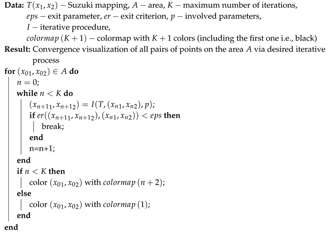
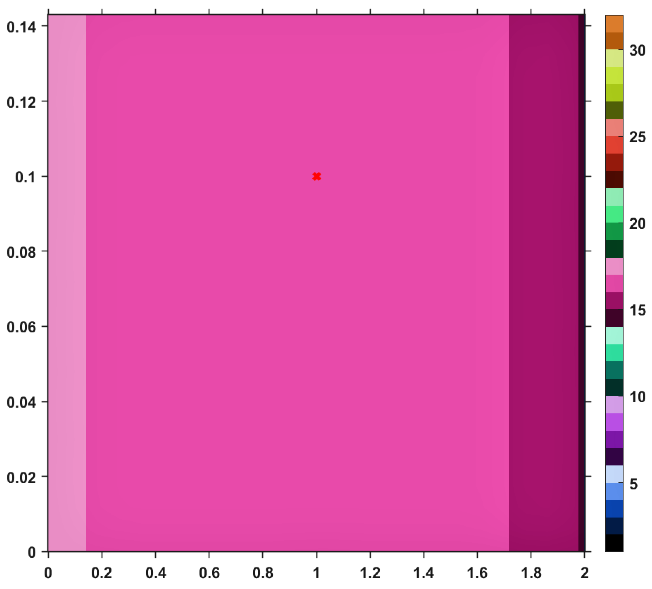
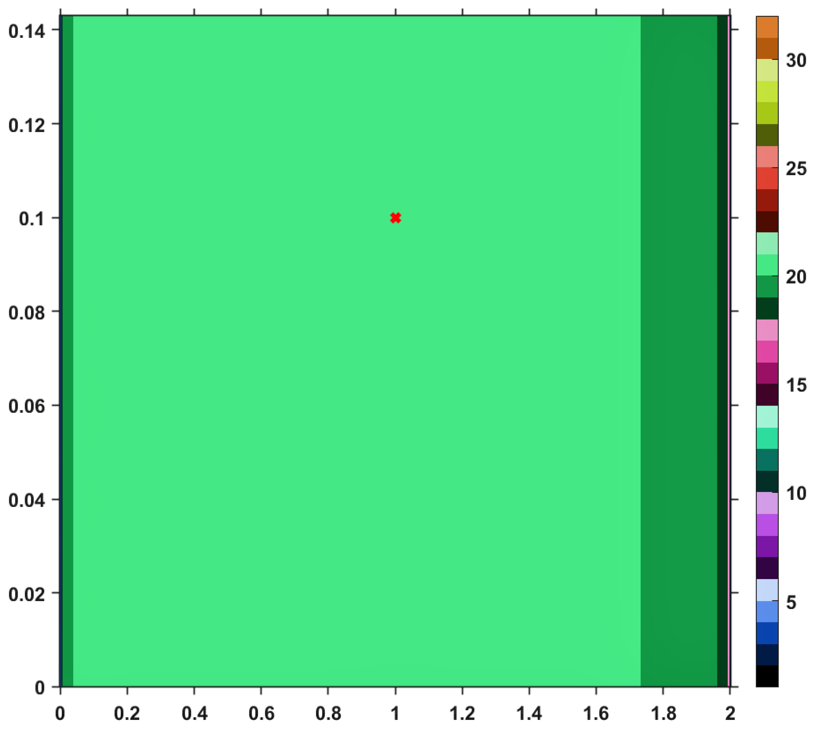
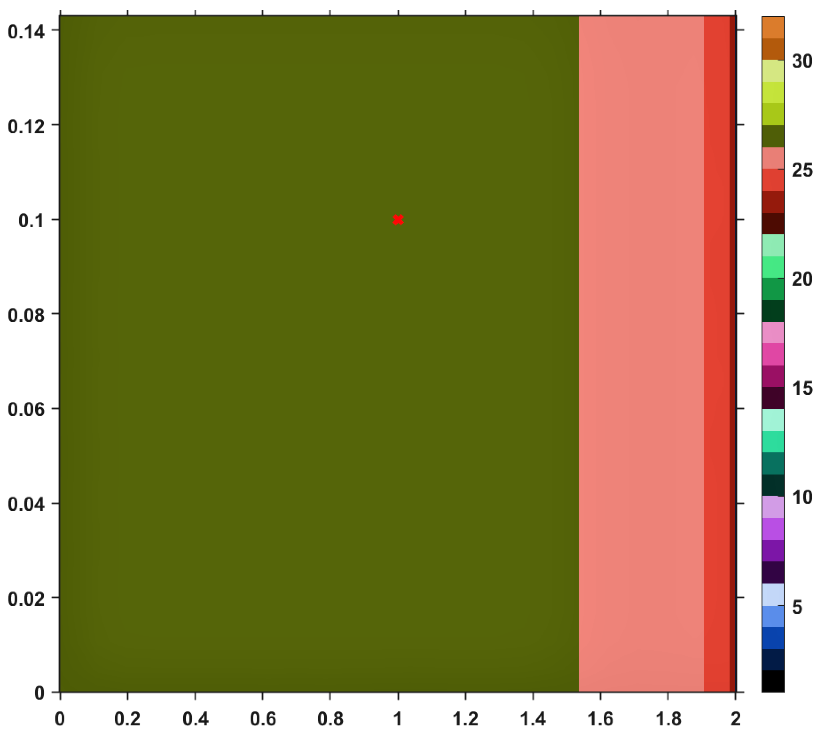
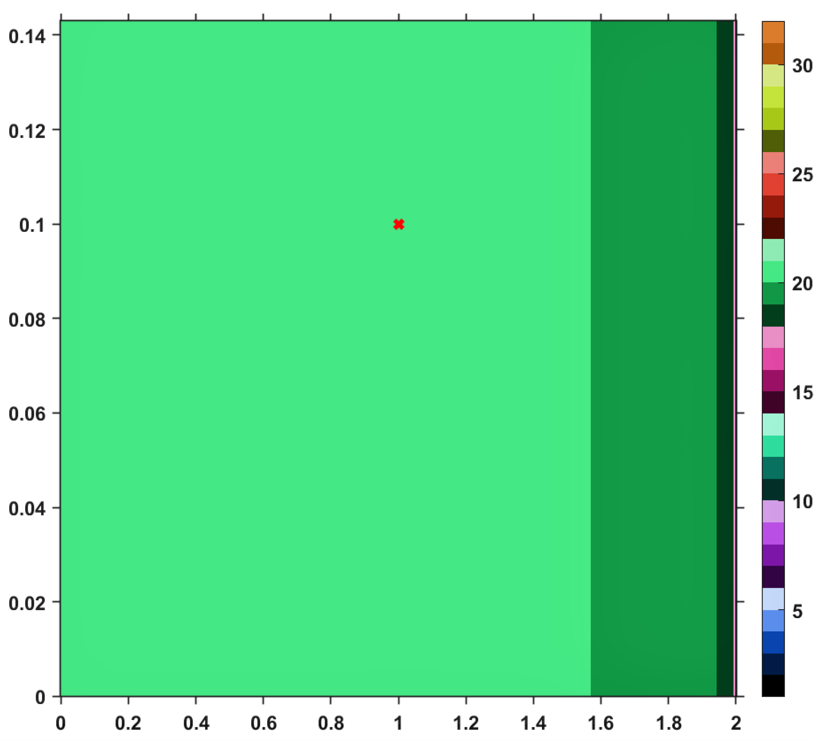
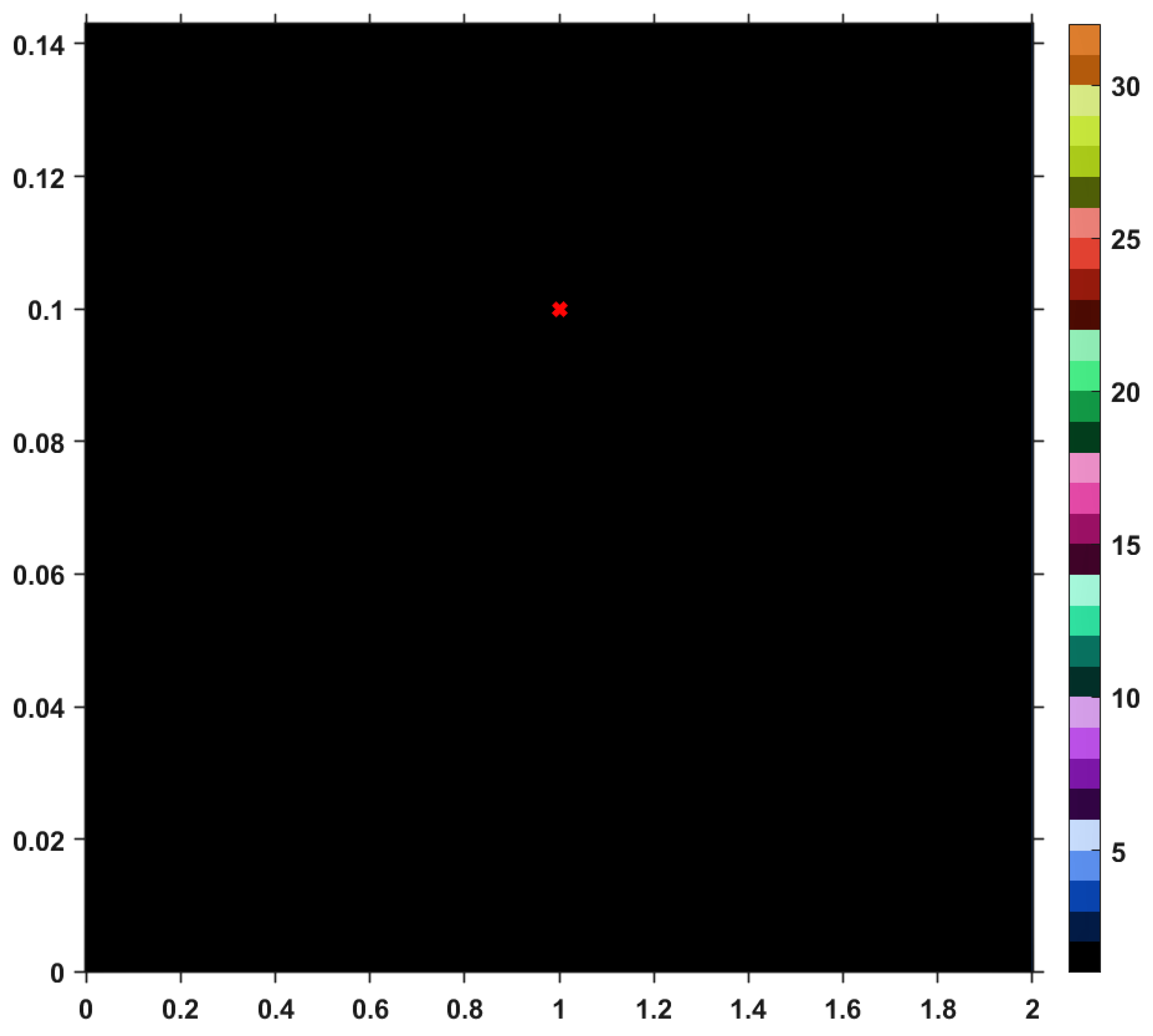
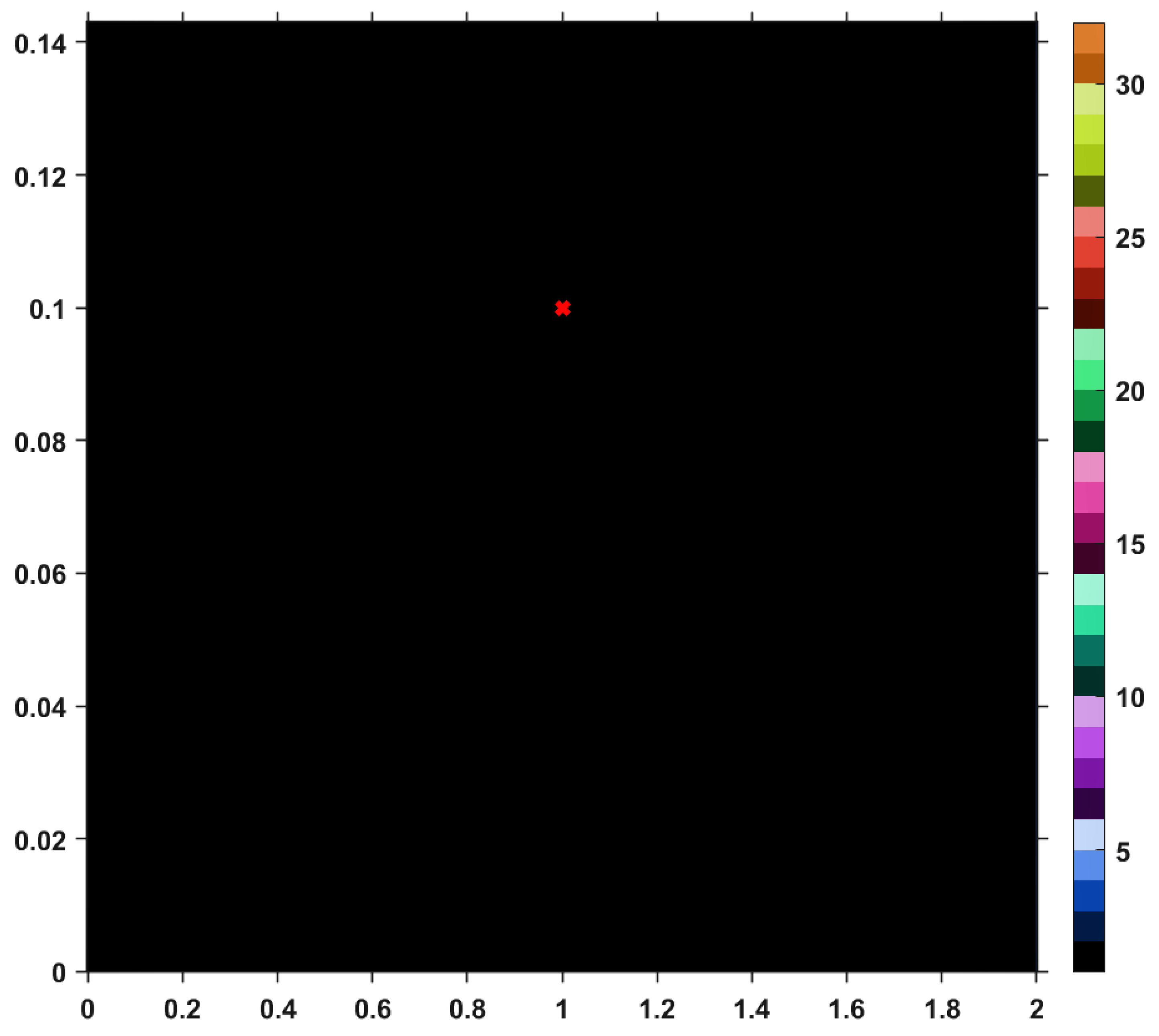
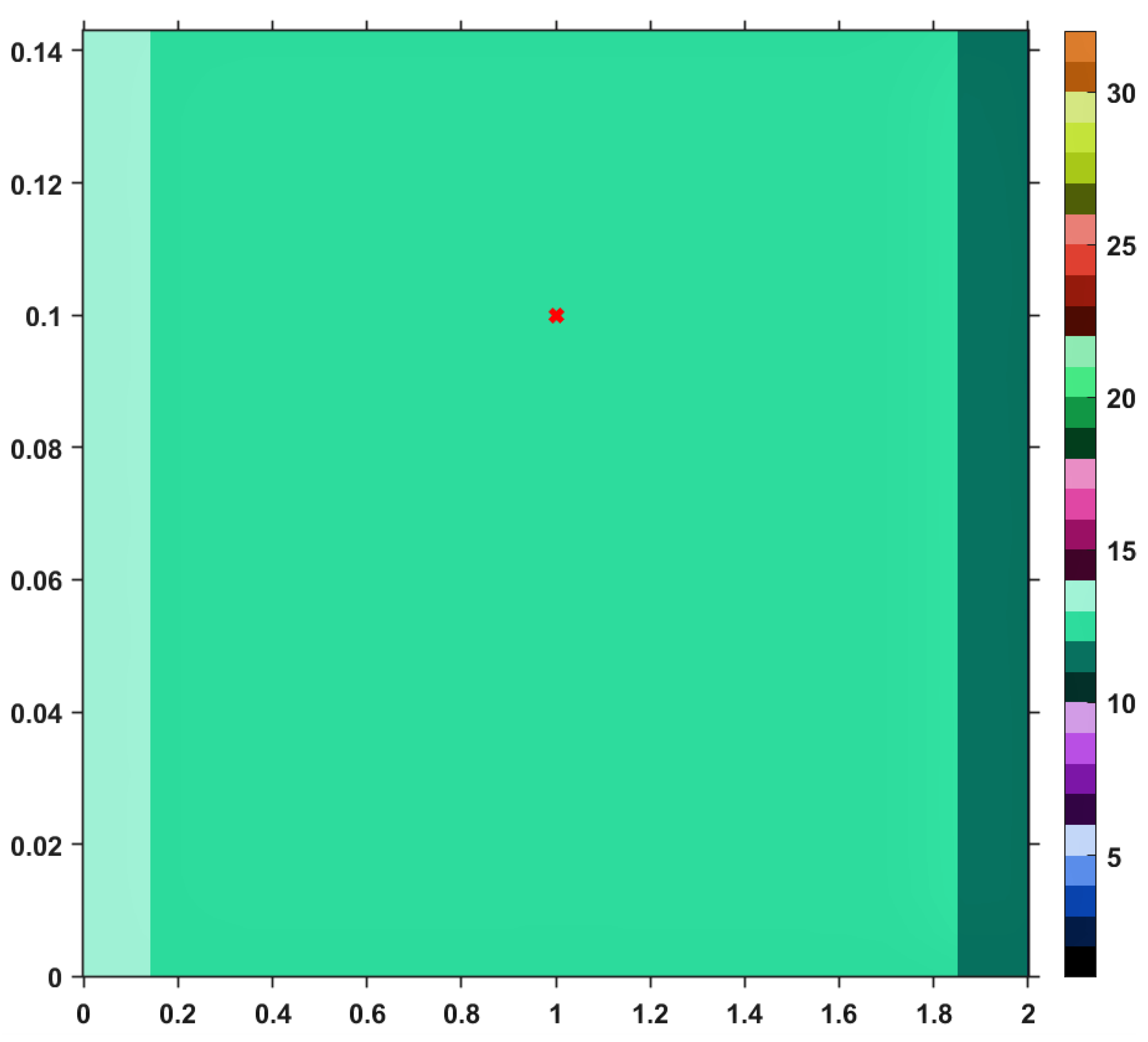
Using this Suzuki mapping and the TTP iteration procedure, along with other iterative schemes mentioned in the first section, let us visualize (and analyze) the convergence behaviors by performing a numerical simulation. The results are pictured in the images included in Figure 1, Figure 2, Figure 3, Figure 4, Figure 5, Figure 6 and Figure 7. The maximum number of iterations to be performed until the algorithm stops is set to $K=30$ and the exit parameter to $\epsilon ={10}^{-15}$. The $\left[0,2\right]\times \left[{\displaystyle 0,\frac{1}{7}}\right]$ rectangle is represented by an open window having the values of $x_1$ on the horizontal axis and those of $x_2$ on the vertical one. As a general feature of the obtained images, the first color (black) of the right-sided colorbar, corresponds to those pairs of points having long orbits, non-convergent for the maximum number of iterations imposed. Apart from black, each color in the range corresponds to a value between 1 and 30, in ascending order, signifying the number of iterations needed to reach the fixed point of T with the error $\epsilon$. On what concerns the values of the involved parameters, we chose (purely arbitrary) the sequences ${\displaystyle {\alpha }_n=\frac{1}{\sqrt{9n+1}}}$, ${\displaystyle {\beta }_n=\frac{{(2n+1)}^{\frac{1}{3}}}{10n+11}}$ and ${\displaystyle {\gamma }_n=\sqrt{\frac{n}{3n+4}}}$. The Algorithm 1 is used to generate these images and goes through the following steps: first, take a pair of starting points from the area $\left[0,2\right]\times \left[{\displaystyle 0,\frac{1}{7}}\right]$, then choose an iteration procedure and perform it until the maximum number of iteration K is reached or the exit criterion is satisfied (for this case, as we have worked with the Taxicab norm, the exit criterion is ${∥(x_{n_1},x_{n_2})-(x_{{n+1}_1},x_{{n+1}_2})∥}_1=|x_{n_1}-x_{{n+1}_1}|+|x_{n_2}-x_{{n+1}_2}\left|\right)$. When the loop terminates, the program will assign to every starting point from the specified area a pixel and a corresponding color, based on the number of iterations performed.

Algorithm 1: Convergence visualization

Let us take a closer look to the first image; namely, Figure 1, the one corresponding to the TTP iterative process. One can see that, as the set of fixed points is approached, the color becomes darker, meaning that the number of iterations performed decreases. Moreover, the last line of the image takes a dark blue color. This is actually to be expected since that particular line is corresponding to the set of fixed points of T and just one iteration is needed until the exit criterion is satisfied. Similar analyses regarding convergence speed can be realized for the images provided by others iterative processes, i.e., Picard, Mann, Agarwal and Abbas-Nazir. It is interesting to point out that the corresponding images for iterations like Ishikawa and Noor are entirely black, meaning that the procedures are very slowly convergent (they need more than 30 iterative steps) or they do not converge at all. The explanation for such a behavior is that T defined above is a Suzuki-generalized nonexpansive mapping, but it is not nonexpansive. Nevertheless, it is clear that, among all iterative processes, TTP remains one of the fastest; it is only surpassed by he Abbas-Nazir procedure. This last statement is also emphasized on the

Table 1. Number of iterative steps required for approximating a fixed point, with error $\epsilon ={10}^{-15}$, starting from the initial point $(x_1^{*},x_2^{*})=(1,0.1)$.

	TTP	Picard	Mann	Ishikawa	Agarwal	Noor	Abbas-Nazir
(1, 0.1)	15	19	25	-	19	-	11

, by taking a random point from the domain of T ($(x_1,x_2)=(1,0.1)$, also marked on each image with a red ’x’) and listing the number of iterations needed to approximate the fixed point $(x_1^{*},x_2^{*})=(1,0.1)$ for each iteration procedure.

In the following, we provide a second example of a Suzuki mapping which is not nonexpansive, on a function space. This is meant to strengthen the assertion that mappings satisfying condition C is indeed a wide class of operators, and examples for it can be provided both on $\mathbb{R}$ (see [15]) and ${\mathbb{R}}^2$, as well as on infinite dimensional spaces.

Example 2.

Consider the Banach space $X=L^{\infty }\left(\mathbb{R}\right)$ of all essentially bounded Lebesgue measurable functions, endowed with the essential supremum norm

$${∥f∥}_{\infty }={\mathrm{ess}\sup }_{\mathbb{R}}\left|f\right|=inf\{M:|f\left(x\right)|\le Ma.e.on\mathbb{R}\}.$$

Let $C=\{f:\mathbb{R}\to [0,7]:f(x)=f(0),\forall x\le 0\}$ and

$$T:C\to C,Tf\left(x\right)=\left\{\begin{array}{cc}f\left(x\right),& x>0\\ {\displaystyle \frac{2}{7}f\left(0\right),}& x\le 0,f\left(0\right)\ne 7\\ 3,& x\le 0,f\left(0\right)=7.\end{array}\right.$$

We shall further prove that T mentioned above is an example of a Suzuki-generalized nonexpansive mapping.

Proof. 

Suppose the inequality ${\displaystyle \frac{1}{2}{∥f-Tf∥}_{\infty }\le {∥g-f∥}_{\infty }}$ is satisfied. This is further equivalent with ${\displaystyle \frac{1}{2}\left|Tf\left(0\right)-f\left(0\right)\right|\le max\left\{\left|f\left(0\right)-g\left(0\right)\right|,{\mathrm{ess}\sup }_{(0,\infty )}\left|f\left(x\right)-g\left(x\right)\right|\right\}}$. Thus, two cases arise:

Case 1: Let us presume that $max\left\{\left|f\left(0\right)-g\left(0\right)\right|,{\mathrm{ess}\sup }_{(0,\infty )}\left|f\left(x\right)-g\left(x\right)\right|\right\}=\left|f\left(0\right)-g\left(0\right)\right|$. For T to satisfy condition $\left(C\right)$, this must imply $max\left\{\left|Tf\left(0\right)-Tg\left(0\right)\right|,{\mathrm{ess}\sup }_{(0,\infty )}\left|Tf\left(x\right)-Tg\left(x\right)\right|\right\}\le \left|f\left(0\right)-g\left(0\right)\right|$. Because of this last inequality, it is expected the problem to be divided again into two sub-cases. We will analyze just the nontrivial one i.e., ${\displaystyle \frac{1}{2}\left|Tf\left(0\right)-f\left(0\right)\right|\le \left|f\left(0\right)-g\left(0\right)\right|}$ implies $\left|Tf\left(0\right)-Tg\left(0\right)\right|\le \left|f\left(0\right)-g\left(0\right)\right|$, as the desired result follows easly from the other one. If $f\left(0\right)\ne 7$ and $g\left(0\right)\ne 7$, or $f\left(0\right)=7$ and $g\left(0\right)=7$, it can be easly noticed that T is nonexpansive, and therefore condition $\left(C\right)$ is automatically fulfilled. For $f\left(0\right)\ne 7$ and $g\left(0\right)=7$, T is nonexpansive just for $f\left(0\right)\in \left[{\displaystyle 0,\frac{28}{5}}\right]$, and again, condition $\left(C\right)$ is satisfied. For $f\left(0\right)\in \left({\displaystyle \frac{28}{5},7}\right)$ and $g\left(0\right)=7$, ${\displaystyle \frac{1}{2}\left|Tf\left(0\right)-f\left(0\right)\right|\le \left|f\left(0\right)-g\left(0\right)\right|}$ becomes ${\displaystyle \frac{5f\left(0\right)}{14}\le 7-f\left(0\right)}$ which is not true as ${\displaystyle \frac{5f\left(0\right)}{14}\in \left({\displaystyle 2,\frac{5}{2}}\right)}$ and $7-f\left(0\right)\in \left({\displaystyle 0,\frac{7}{5}}\right)$. The same result is obtained if we take $f\left(0\right)=7$ and $g\left(0\right)\ne 7$. Considering all the situations analyzed, we conclude that T is a Suzuki-mapping for the current case.

Case 2: Suppose $max\left\{\left|f\left(0\right)-g\left(0\right)\right|,{\mathrm{ess}\sup }_{(0,\infty )}\left|f\left(x\right)-g\left(x\right)\right|\right\}={\mathrm{ess}\sup }_{(0,\infty )}\left|f\left(x\right)-g\left(x\right)\right|$. The inequality ${\displaystyle \frac{1}{2}\left|Tf\left(0\right)-f\left(0\right)\right|\le {\mathrm{ess}\sup }_{(0,\infty )}\left|f\left(x\right)-g\left(x\right)\right|}$ must imply $max\left\{\left|Tf\left(0\right)-Tg\left(0\right)\right|,{\mathrm{ess}\sup }_{(0,\infty )}\left|Tf\left(x\right)-Tg\left(x\right)\right|\right\}\le {\mathrm{ess}\sup }_{(0,\infty )}\left|f\left(x\right)-g\left(x\right)\right|$. If we consider that $\left|Tf\left(0\right)-Tg\left(0\right)\right|\le {\mathrm{ess}\sup }_{(0,\infty )}\left|f\left(x\right)-g\left(x\right)\right|$, it follows ${∥Tf-Tg∥}_{\infty }={\mathrm{ess}\sup }_{(0,\infty )}\left|f\left(x\right)-g\left(x\right)\right|$; but as $\left|f\left(0\right)-g\left(0\right)\right|\le {\mathrm{ess}\sup }_{(0,\infty )}\left|f\left(x\right)-g\left(x\right)\right|$, it follows that ${∥f-g∥}_{\infty }={\mathrm{ess}\sup }_{(0,\infty )}\left|f\left(x\right)-g\left(x\right)\right|$ too, so T is nonexpansive. If we suppose $\left|Tf\left(0\right)-Tg\left(0\right)\right|>{\mathrm{ess}\sup }_{(0,\infty )}\left|f\left(x\right)-g\left(x\right)\right|$, kipping in mind that ${\mathrm{ess}\sup }_{(0,\infty )}\left|f\left(x\right)-g\left(x\right)\right|\ge \left|f\left(0\right)-g\left(0\right)\right|$ on one side, ${\displaystyle {\mathrm{ess}\sup }_{(0,\infty )}\left|f\left(x\right)-g\left(x\right)\right|\ge \frac{1}{2}\left|Tf\left(0\right)-f\left(0\right)\right|}$ on the other side and considering all combinations that T could involve, we find that the assumption is absurd and $\left|Tf\left(0\right)-Tg\left(0\right)\right|$ could not be grater than ${\mathrm{ess}\sup }_{(0,\infty )}\left|f\left(x\right)-g\left(x\right)\right|$. So, overall, T is a Suzuki mapping in Case 2 also. □

6. Conclusions

This paper analyzes a three-steps Thakur iterative procedure in connection with mappings satisfying Suzuki’s generalized nonexpansiveness condition, known as property $\left(C\right)$. A necessary and sufficient condition regarding the existence of fixed points for Suzuki mappings is stated and proved via the TTP iterative process. Furthermore, convergence results are obtained when additional hypotheses related to Opial’s property, compactness or condition $\left(I\right)$ are assumed. Fresh examples of Suzuki mappings which are not nonexpansive are further provided; the settings for these examples are ${\mathbb{R}}^2$, with the Taxicab norm, and $L^{\infty }\left(\mathbb{R}\right)$ endowed with the essential supremum norm. But, the most interesting feature about the example in ${\mathbb{R}}^2$ is a numerical simulation, resulting in a visual comparative analysis of the convergence behaviors of several iteration procedures. This numerical modeling uses similar techniques as the root-finding procedures for complex polynomials, which ultimately led to polynomiographic visualization.

Overall, the novelty of this paper is twofold. First, a new perspective on the TTP iteration procedure is provided; this iterative scheme was originally conceived as a tool in connection with nonexpansive mappings; now, it is proved to be an instrument as good as before for reaching the fixed points of Suzuki mappings too. Moreover, having in mind the computational dimension of an iteration procedure, a data dependency analysis is convenient, since errors can occur when using computer programs. Usually, this constrains us to actually use a perturbed mapping $\tilde{T}$, instead of the theoretical one. We managed to prove that a small perturbation of the initial data does not significantly affect the computational process of the fixed point of a contractive operator.

Secondly, more complex examples of Suzuki mappings are provided. Picking ${\mathbb{R}}^2$ as the setting, an interesting visual procedure is suggested as a possible new approach related to convergence analysis. In addition, another example proves that one could easily exceed the framework of finite dimensional normed spaces.

References

1. Krasnoselskii, M.A. Two remarks on the method of succesive approximations. Uspekhi Math. Nauk. 1955, 10, 123–127. (In Russian) [Google Scholar]
2. Mann, W.R. Mean value methods in iteration. Proc. Am. Math. Soc. 1953, 4, 506–510. [Google Scholar] [CrossRef]
3. Ishikawa, S. Fixed points by a new iteration method. Proc. Am. Math. Soc. 1974, 44, 147–150. [Google Scholar] [CrossRef]
4. Agarwal, R.P.; O’Regan, D.; Sahu, D.R. Iterative construction of fixed points of nearly asymptotically nonexpansive mappings. J. Nonlinear Convex Anal. 2007, 8, 61–67. [Google Scholar]
5. Noor, M.A. New approximation schemes for general variational inequalities. J. Math. Anal. Appl. 2000, 251, 217–229. [Google Scholar] [CrossRef]
6. Abbas, M.; Nazir, T. A new faster iteration process applied to constrained minimization and feasibility problems. Mat. Vesn. 2014, 66, 223–234. [Google Scholar]
7. Thakur, B.S.; Thakur, D.; Postolache, M. A new iterative scheme for approximating fixed points of nonexpansive mappings. Filomat 2016, 30, 2711–2720. [Google Scholar] [CrossRef]
8. Thakur, D.; Thakur, B.S.; Postolache, M. New iteration scheme for numerical reckoning fixed points of nonexpansive mappings. J. Inequal. Appl. 2014, 328. [Google Scholar] [CrossRef]
9. Browder, F.E. Nonexpansive nonlinear operators in Banach space. Proc. Natl. Acad. Sci. USA 1965, 54, 1041–1044. [Google Scholar] [CrossRef]
10. Kirk, W.A. A fixed point theorem for mappings wich do not increase distances. Am. Math. Mon. 1965, 72, 1004–1006. [Google Scholar] [CrossRef]
11. Suantai, S.; Donganont, M.; Cholamjiak, W. Hybrid methods for a countable family of G-nonexpansive mappings in Hilbert spaces endowed with graphs. Mathematics 2019, 7, 936. [Google Scholar] [CrossRef]
12. Suzuki, T. Fixed point theorems and convergence theorems for some generalized nonexpansive mappings. J. Math. Anal. Appl. 2008, 340, 1088–1095. [Google Scholar] [CrossRef]
13. Abkar, A.; Eslamian, M. A fixed point theorem for generalized nonexpansive multivalued mappings. Fixed Point Theory 2011, 12, 241–246. [Google Scholar]
14. Dhompongsa, S.; Inthakon, W.; Kaewkhao, A. Edelstein’s method and fixed point theorems for some generalized nonexpansive mappings. J. Math. Anal. Appl. 2009, 350, 12–17. [Google Scholar] [CrossRef]
15. Thakur, B.S.; Thakur, D.; Postolache, M. A new iterative scheme for numerical reckoning fixed points of Suzuki’s generalized nonexpansive mappings. Appl. Math. Comput. 2016, 275, 147–155. [Google Scholar] [CrossRef]
16. Zuo, Z.; Cui, Y. Iterative approximations for generalized multivalued mappings in Banach spaces. Thai J. Math 2011, 9, 333–342. [Google Scholar]
17. Bejenaru, A.; Postolache, M. On Suzuki mappings in modular spaces. Symmetry 2019, 11, 319. [Google Scholar] [CrossRef]
18. Garcia-Falset, J.; Llorens-Fuster, E.; Suzuki, T. Fixed point theory for a class of generalized nonexpansive mappings. J. Math. Anal. Appl. 2011, 375, 185–195. [Google Scholar] [CrossRef]
19. Bejenaru, A.; Postolache, M. Generalized Suzuki-type mappings in modular vector spaces. Optimization 2019. [Google Scholar] [CrossRef]
20. Goebel, K.; Kirk, W.A. Topic in Metric Fixed Point Theory; Cambridge University Press: Cambridge, UK, 1990. [Google Scholar]
21. Schu, J. Weak and strong convergence of fixed points of asymptotically nonexpansive mappings. Bull. Austral. Math. Soc. 1991, 43, 153–159. [Google Scholar] [CrossRef]
22. Edelstein, M. Fixed point theorems in uniformly convex Banach spaces. Proc. Am. Math. Soc. 1974, 44, 369–374. [Google Scholar] [CrossRef]
23. Opial, Z. Weak convergence of the sequence of succesive approximations for nonexpansive mappings. Bull. Am. Math. Soc. 1967, 73, 595–597. [Google Scholar] [CrossRef]
24. Senter, H.F.; Dotson, W.G. Approximating fixed points of nonexpansive mappings. Proc. Am. Math. Soc. 1974, 44, 375–380. [Google Scholar] [CrossRef]
25. Berinde, V. Iterative Approximation of Fixed Points; Springer: Berlin, Germany, 2007. [Google Scholar]
26. Soltuz, S.M.; Grosan, T. Data dependence for Ishikawa iteration when dealing with contractive like opeartors. Fixed Point Theory Appl. 2008, 242916, 1–7. [Google Scholar]
Figure 1. TTP.
Symmetry 11 01441 g001
Figure 2. Picard.
Symmetry 11 01441 g002
Figure 3. Mann.
Symmetry 11 01441 g003
Figure 4. Agarwal.
Symmetry 11 01441 g004
Figure 5. Ishikawa.
Symmetry 11 01441 g005
Figure 6. Noor.
Symmetry 11 01441 g006
Figure 7. Abbas-Nazir.
Symmetry 11 01441 g007