1. Introduction
Internet and software technologies have developed considerably over the last decade. With the increasing complexity of user requirements, software system architecture has evolved from a monolithic system to today’s cloud-native architecture. With emerging container technologies, container-based cloud application architecture has become the most popular software architecture. Although cloud-native architecture has numerous benefits, such as high availability and high scalability, the management and maintenance of cloud applications present a new challenge, and the dependability of cloud applications has become a major concern for application providers. Anomalies, such as resource competition for concurrent requests and deadlock, must be accompanied by other symptoms before they occur. In fact, these anomalies can often be characterized by outliers in performance metrics. If these anomalies are not found and solved in time, they will eventually lead to service failures and business losses. Therefore, real-time anomaly detection and alarms for cloud applications are necessary.
This paper presents KPI-TSAD, a novel anomaly detection approach for time-series data that contain both spatial features and temporal features. Furthermore, KPI-TSAD includes a novel oversampling method based on VAE that could reasonably expand the minority class sample and fit its probability distribution function without any prior assumption regarding real distribution, allowing KPI-TSAD to attain good generalization capabilities in data-scarce scenarios where fewer training data are available.
1.1. Background
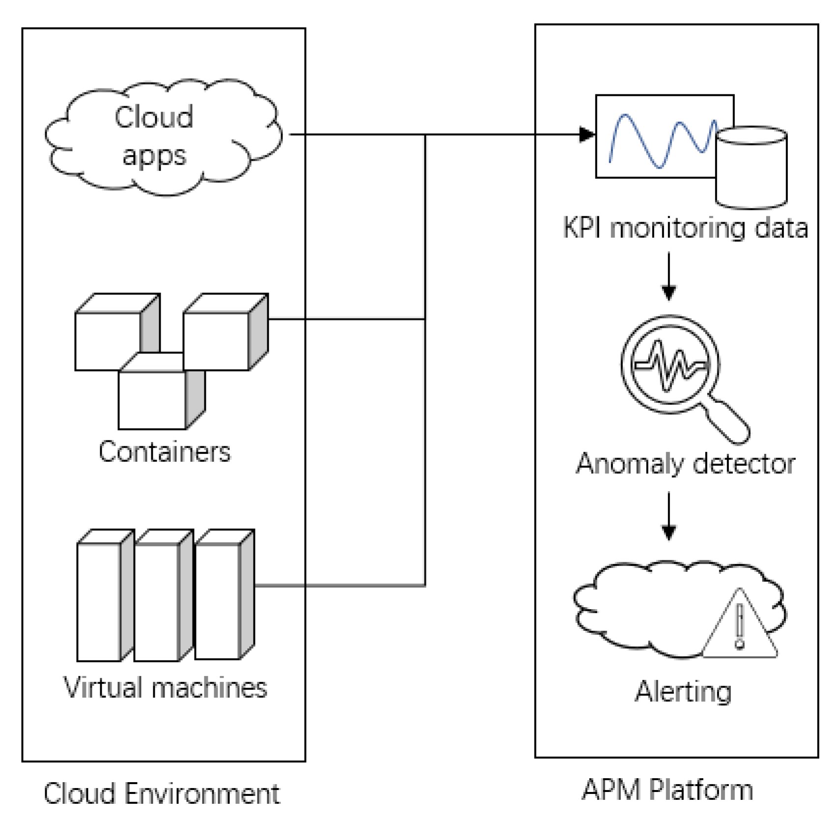
To deliver a great digital customer experience, application performance management (APM) solutions monitor and manage the performance and availability of software applications. As shown in
Figure 1, the anomaly detector plays a critical role in the APM platform; its performance has a direct effect on the accuracy of the alerting system. At present, a false alarm from the APM system is the most critical problem.
The performance issues of cloud applications are usually accompanied by some unusual behavior. Traditional methods for performance anomaly detection based on thresholds and rules work well for key performance indicators (KPIs), which are generally within a narrow range of predictable values.
However, not all of the alerting problems are solvable using the threshold-based anomaly detection approach. For example, disks’ running out of space is a classic noisy alert in a number of environments. To be more specific, it happens when disks reach the typical 95% threshold and then drop back below it by themselves multiple times every day. Otherwise, they remain at 98%, which is acceptable, or they go from 5% to 100% in a matter of minutes. However, these problems are not caused by the threshold being set to the wrong value or by the operator’s need for adaptive self-learning behavior. The problem is sending an alert at the predicted time when a disk runs out of space instead of alerting when it is full. There are three important aspects that assure accurate and non-noised anomaly detection:
A clear and unambiguous definition of the problem that we seek to detect.
The best indicators for monitoring the problems are usually directly related to one or more business goals or desired outcomes; in other words, KPIs that are related to the actual effect.
The model required to link the system behavior to the anomalous behavior.
In this paper, we focus on a discussion of the third aspect—that is, an anomaly detection model— and it is assumed that the first two aspects have been solved before anomaly detection is addressed.
1.2. Problem Description and Definition
In this study, the identification of anomalies within a single time series was the primary focus, and it was worth noting that the time series concerned was considered to be a continuous sequence of numerical data rather than a discrete sequence of symbolic data that require a different set of methods. Imagine a time series starting from time 0 to time T, i.e., . The time-series anomaly detection identified the set of anomalous points within the time series or labeled all the points within the time series with irrespective of whether their corresponding points were anomalous or not. More formally, the problem could be expressed as follows:
Given: a time series X,
Find: anomalous points in X.
Although the above formulation concerns anomaly detection in a time series that has sequential information among the data points, traditional anomaly detection methods are still applicable. This is achieved through the reduction of the time-series anomaly detection problem. A typical method for problem reduction is time-delay embedding, which adopts a sliding window to construct multivariate data instances from the original time series. For instance, suppose that the size of the sliding window is set as E; then, using the method of time-delay embedding would lead to the establishment of a new dataset from the time series
X as follows:
where
.
Consequently, a time series is converted to a set of multivariate data instances that enable the use of traditional anomaly detection methods. Note that the sequential information within the original time series is encoded within the multivariate data. Therefore, anomaly detection should also take sequential information into consideration.
In this study, we attempted to take an anomaly detection problem as a classification problem to solve. Given a dataset of labeled KPI samples with sliding windows:
where
is the input vector whose components can represent the KPIs.
Y is the output that is the corresponding anomaly label for
, where
, 0 refers to normal status, and the other value
represents the abnormal status. The solution aims to find a suitable model to extrapolate the corresponding value
of any new instance
.
1.3. Contribution and Outlines
With the recent development of deep neural networks, we have been motivated to adopt deep-learning approaches to address the issue of anomaly detection by extracting both temporal and spatial features features of the time-series sequence data [
1]. Therefore, in this study, the structure of neural networks in KPI-TSAD consisted of the CNN and LSTM layers, structured linearly. The convolution and pooling layers were used to extract the spatial features of the data sequence, and the LSTM layers were used to extract the temporal features.
Another critical issue in a classification-based anomaly detection solution is the extreme imbalanced classification problem, as abnormal samples are usually considerably fewer than normal samples. Because of their rarity, the important minority samples are often ignored. Oversampling algorithms could be applied to increase the recognition rate of minority samples by increasing the number of minority samples in the training set. However, traditional oversampling methods fail to utilize fully the information contained in the original samples and scarcely improve the effect of classifying minority samples; therefore, we propose an oversampling model, namely VAEGEN, which uses a variational auto-encoder (VAE) [
2] as a generative model to achieve data augmentation. In summary, this study makes the following contributions:
A novel oversampling model VAEGEN based on VAE was applied to address imbalances in classification. It increases the number of minority samples in the training set to increase their recognition rate. Compared with the traditional oversampling method, this method provides for a more obvious and reasonable improvement of the effect of anomaly detection.
A novel anomaly detector based on deep-learning models with CNN and LSTM neural networks was developed. It effectively models the spatial and temporal information contained in time-series data.
Benchmark-based comparison experiments were conducted. The effectiveness and feasibility of the proposed method was proved by different comparative experiments from different perspectives.
Finally, KPI-TSAD was successfully applied to the time-series anomaly detection of the KPI monitoring data from real production environments. The rest of this paper is organized as follows. In
Section 2, we first review and evaluate the related work. Then, we introduce the proposed anomaly detector KPI-TSAD in
Section 3. Then the evaluation methodology for KPI-TSAD is introduced in
Section 4. In
Section 5 and
Section 6, we present experiments on both Yahoo benchmark datasets and AIOps2018 Challenge KPI datasets and discuss the results. In
Section 7, we draw the conclusion and discuss future work.
2. Related Works
In this section, we review and discuss the related works on time-series anomaly detection and oversampling techniques for imbalanced time-series learning. In general, we attempt to classify the time-series anomaly detection studies into four categories: statistical prediction methods, time-series decomposition methods, state-transition models, and deep-learning methods. In addition, we particularly introduce some state-of-the-art methods that are used on Yahoo’s benchmark datasets. Finally, we review two of the most commonly used oversampling methods: SMOTE and ADASYN.
2.1. Statistical Prediction Methods
The statistical prediction methods for anomaly detection mainly concern the predictive models of univariate time series. These models aim at extracting the patterns in a given time series so as to accurately predict the subsequent values. Traditional methods, such as the auto-regressive mode and the moving average model (ARIMA), are statistical analysis methods that are potent in modeling univariate time series for prediction. More advanced methods have rapidly emerged in recent years. In the recent literature, many different time-series anomaly detection detectors have been studied on the basis of traditional statistical models (e.g., [
3,
4,
5,
6]), and most of these detectors were developed to calculate anomaly scores. As these algorithms generally contain simple assumptions for the applicable KPIs, effort needs to be made to select a suitable detector for a given KPI, and then, the detectors’ parameters should be fine-tuned on the basis of the training data. Single integration of these detectors does not work according to Liu et al. [
7] and Laptev et al. [
8]. Therefore, these detectors are not widely used in practice.
2.2. Time-Series Decomposition Methods
Typical time-series decomposition methods include additive decomposition, multiplicative decomposition, X-12-ARIMA decomposition, and STL [
9], which is a primary technique to achieve the decomposition of seasonal information, which supports effective long-term time-series anomaly detection. Time-series decomposition is an excellent tool for preprocessing time series for further applications. It is widely adopted, particularly when analyzing time series with a growing trend or a strong periodicity. Nonetheless, for time series with no explicit periodicity, time-series decomposition may incur additional work and may not assist on the time-series anomaly detection.
2.3. State-Transition Models
State-transition models are methods that examine the dynamic state transitions within a system or a time series. In these models, a time series is assumed to maintain a steady-state transition pattern that can be modeled as a stable property. This stable model is normally realized as a Markov model, a hidden Markov model (HMM) [
10], or a finite-state machine (FSM) [
11]. Over the years, numerous studies have been undertaken to exploit the state-transition models for sequential-data anomaly detection. In 2015, Görnitz et al. [
12] proposed a hidden Markov anomaly detector that has been shown to outperform the one-class support vector machine (SVM) in situations where the data contain latent dependency structures. Additionally, in [
13], a timed automaton was used to profile the normal sequential behavior of a digital video broadcasting system for the purpose of anomaly detection. All of these works demonstrate the effectiveness of state-transition models in analyzing sequential data.
2.4. Deep-Learning Methods
With the development of deep-learning networks, many researchers have sought to use them to extract the hidden features in the data. Anomaly detection solutions could be categorized into two classes [
14]: (1) supervised anomaly detection; and (2) unsupervised anomaly detection. Supervised anomaly detection is fundamentally a classification problem that endeavors to distinguish abnormality from normality. In contrast, unsupervised anomaly detection does not require access to the exact labels of the given dataset. It achieves anomaly detection by identifying the shared patterns among the data instances and by observing the outliers. Hence, unsupervised anomaly detection is usually concerned with outlier detection.
2.4.1. Supervised Approaches
Specific methods for supervised anomaly detection, i.e., classification-based anomaly detection, can be found in other related studies [
15,
16,
17]. Supervised ensemble approaches, Opprentice [
7] and EGADS [
8], were proposed to avoid the complicated algorithm/parameter tuning when traditional statistical anomaly detectors are used. By taking traditional detectors’ anomaly scores as features and user feedbacks as labels, they can provide training for anomaly classifiers.
2.4.2. Unsupervised Approaches
In recent years, it has become a popular trend to carry out anomaly detection by adopting unsupervised machine learning algorithms, such as one-class SVM [
18,
19], and clustering-based methods, such as KDE [
20], VAE [
21], and VRNN [
22]. The principle is to focus on normal patterns rather than anomalies: models can be trained at any time, even without labels, because the KPIs usually consist of normal data. In general, these models first recognize the normal regions that are in the original or potential feature space and then measure the distance between an observation and the normal regions to rate the anomaly scores.
A recent study by Roggen et al. [
23] utilized a neural network architecture combining convolutional and recurrent layers to identify and extract relevant features from multivariate sensor data, which also revealed that CNNs are proven to excel at extracting features from grid-like input structures. Further, RNNs have shown good results in handling temporal features. The method proposed in this paper is a supervised learning method. Compared with traditional machine learning algorithms, the proposed convolutional LSTM architecture obviously achieved better results, although the classifier received training on raw input sequences and had no further feature engineering.
2.5. State-of-The-Art Methods for Comparison
Considering that we were using public benchmark datasets, we decided to conduct comparative experiments with some state-of-the-art methods that previous researchers have applied to the same benchmark datasets. Both Twitter’s anomaly detection package and Yahoo’s extensible generic anomaly detection system (EGADS) were used in a recent study [
24], in which DeepAnT was also proposed as an unsupervised time-series anomaly detection method. Based on the seasonal hybrid ESD (S-H-ESD) algorithm, Twitter Inc. open-sourced its own anomaly detection package in 2015 [
25]. Twitter’s anomaly detection is often used to detect local and global anomalies. Yahoo Labs released EGADS [
8], which is another anomaly detection method that can detect anomalies in large-scale time-series data. EGADS consists of two parts: the anomaly detection module (ADM) and the time-series modeling module (TMM). For a given time series, TMM is used to model the time series and obtain an expected value at timestamp
t. When using ADM, a comparison between the expected value and the actual value is made, and the number of errors
E is calculated. The automatic threshold depends on
E, and the most probable anomalies are obtained. TMM and three anomaly detection models support seven time-series models.
2.6. Oversampling for Imbalanced Time Series
Randomly sampling and replacing the currently available samples is a straightforward method to generate new samples and solve the problem of imbalanced classification. Currently, some popular oversampling solutions focus mainly on getting synthetic samples to obtain the minority-class data, in order to solve the problem of two-class imbalanced classification. The adaptive synthetic (ADASYN) and synthetic minority over-sampling techniques (SMOTE) are widely used for oversampling minority classes [
26]. SMOTE can select all the positive samples and generate synthetic samples in an even manner from the selected seed samples. Relying on an adaptive approach, ADASYN determines the number of synthetic samples to be generated according to the proportion of the surrounding negative samples of each positive sample. With respect to providing a detailed description of these interpolation-based methods and outlining their technical differences, SMOTE would connect the outliers and the inliers, while ADASYN would focus solely on the outliers, and both of them might create a sub-optimal decision function. Furthermore, SMOTE can generate samples through three additional means. By focusing on samples that are close to the optimal decision function, these methods will generate samples in the opposite direction of the nearest neighborhood class. However, traditional oversampling methods fail to utilize fully the information contained in the original samples; they can hardly improve the classification of minority samples. In this study, the proposed VAE oversampling method used the distribution information of the minority samples; adopted a variational auto-encoder to match them to their probability distribution function, without any prior assumption; and expanded the minority sample set to a reasonable extent.
3. Proposed Anomaly Detector
In this section, we introduce the overall workflow and the internal structure of KPI-TSAD. As shown in
Figure 2, first, we processed the imbalanced input time-series data with a sliding window before passing them to the anomaly detector model. Then, we applied the VAEGEN oversampling method to build a balanced dataset, before training the anomaly detection model with the CNN and LSTM networks. Finally, a Softmax function with cross-entropy loss was applied for the classification.
3.1. Data Processing
3.1.1. Preprocess the Input Data
To model temporal relationships in machine learning, a common approach is to use the so-called sliding window of a fixed length l, which creates feature vectors of length l. We took a window of a particular size, slid it through the sequences with a certain padding k (so that its starting point could iterate through the entire file), and output the data sequences of the window size. When applied to a time series or sequence of length N in the form , the sliding window created for each instance , when the padding value was set as 1. Matrix X was composed of the transposed inputs , one vector per row. The abnormal label was denoted as vector Y, once a sequence had an abnormal record; when the sequence was abnormal, the following pseudo-code in Algorithm 1 presents the process details.
| Algorithm 1: Preprocess the time-series input with sliding window. |
Input: raw sequence s, sliding window size l, padding k Output: Initialize X,Y ← values from raw time series s ← labels from raw time series s ← length of raw sequence for i in (0, − l) step with k do Initialize a new sequence list Initialize ← 0 for j in (0, l) do ← append to if then ← 1 end if end for append to X append to Y end for return
|
3.1.2. VAE-Based Oversampling Approach
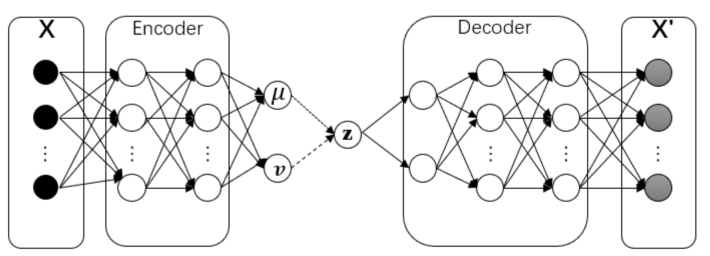
Given there is a sufficient number of anomalous samples in a dataset, the data can be labeled as belonging to either the normal or the anomalous class. In practice, anomaly detection suffers from an extremely unbalanced dataset, where only a few labeled anomalies are available. In this subsection, we introduce the implementation of a new oversampling method VAEGEN based on VAE, which helps to solve the imbalanced classification problem. VAE is also a type of auto-encoder model;
Figure 3 presents its network structure.
In general, the components of each variational auto-encoder include a
, an
, and a
. Input data
X are compressed into a latent space
z by the encoder. The decoder attempts to reconstruct the data, forming a hidden representation. A neural network with
X may constitute the encoder
e. Its output is a hidden representation
z with weights and biases
; that is, the input
X is encoded into a latent representation space
z. Moreover, the space is stochastic and lower-dimensional with a Gaussian probability density. Samples can be collected from this distribution to obtain a representation of
z’s noisy values. Therefore, we denoted the encoder as
. The
is another neural net that decodes the hidden representation
z to a probability distribution of the data with weights and biases
; therefore, we denoted the decoder as
, where
p obeyed an normal distribution with mean
and variance
, that is,
. The variational auto-encoder’s loss function was used to measure the information loss during the reconstruction process. It introduced the effectiveness of the decoder in reconstructing an input image
x and its latent representation
z. First, the loss function was decomposed into terms that had a dependency on a single datapoint
. Then,
was used to refer to the total loss for
N number of data points, while the loss function
for data points
could be denoted as Equation (
3). Gradient descent was adopted to train the variational auto-encoder and improve the loss while considering the parameters of the encoder and the decoder
and
.
The first term is the expected negative log-likelihood of the ith data point or the reconstruction loss. The expectation was related to the encoder’s distribution over the representations. This term encouraged the decoder to learn how to reconstruct the data. If the decoder’s output failed to reconstruct the data well, statistically, it could be said that the decoder showcased the likelihood distribution that did not apply a considerable probability mass to the true data. The second term is the Kullback–Leibler (KL) difference between and , which are the encoder’s distribution. The KL divergence was used to measure the amount of lost information when q was used to represent p, as well as the distance between q and p.
| Algorithm 2: VAE_Model: The VAE modeling algorithm. |
Input: dimension i for input layer, dimension j for intermediate hidden layer, dimension k for hidden layer for latent space
Output: VAE model M, Encoder E, Decoder D
▹ begin to create the encoder network x ← create the input layer with i units ← create the first hidden encoder layer with j units by passing x into it. ← create the second hidden encoder layer with j units by passing into it. ← create the hidden layer with k units by passing into it. represent the mean values for the latent space z when running Gauss sampling. ← create the hidden layer with k units by passing into it. represent the variance values for the latent space z when running Gauss sampling. z ← construct the latent space by sampling from a Gauss distribution with and . E ← build the encoder model with x and ▹ begin to create the decoder network y ← create the input layer with i units ← create the first hidden decoder layer with j units by passing y into it. ← create the second hidden decoder layer with j units by passing the output of into it. ← create the output decoder layer with j units by passing the output of into it. D ← build the decoder model with y and ← decode the latent variables z by passing the latent z from the encoder to the decoder network D. M ← build the VAE model with the encoder input x and the decoder output fit VAE model M with the loss function as denoted in Equation ( 3) returnE,D,M
|
As shown in Algorithm 2, we initially defined a VAE model, where the inputs were the dimension settings for the layers in the VAE auto-encoder networks. When the VAE model M was successfully trained, the decoder D was also trained. VAEGEN used the decoder model D for oversampling, Algorithm 3 is the pseudo-code implementation of VAEGEN. The inputs of the VAEGEN algorithm were the input time-series KPI values X and the corresponding labels Y, while the parameter R denoted the oversampling rate.
| Algorithm 3: VAEGEN: VAE based Oversampling algorithm. |
Input: KPI values X, KPI labels Y, Oversampling rate R, The decoder D from VAE model
Output: KPI values after oversamling, KPI labels after oversampling
← length of X ← multiplied by R , ← split X, Y as training set and validation set , ← filter the abnormal samples from , respectively D ← create a decoder by fitting M with and ← generate samples from a standard normal distribution ← generate oversampling data by passing the into the decoder D ← concatenate the and the original input X ← concatenate the numbers of “1” with original input labels Y return,
|
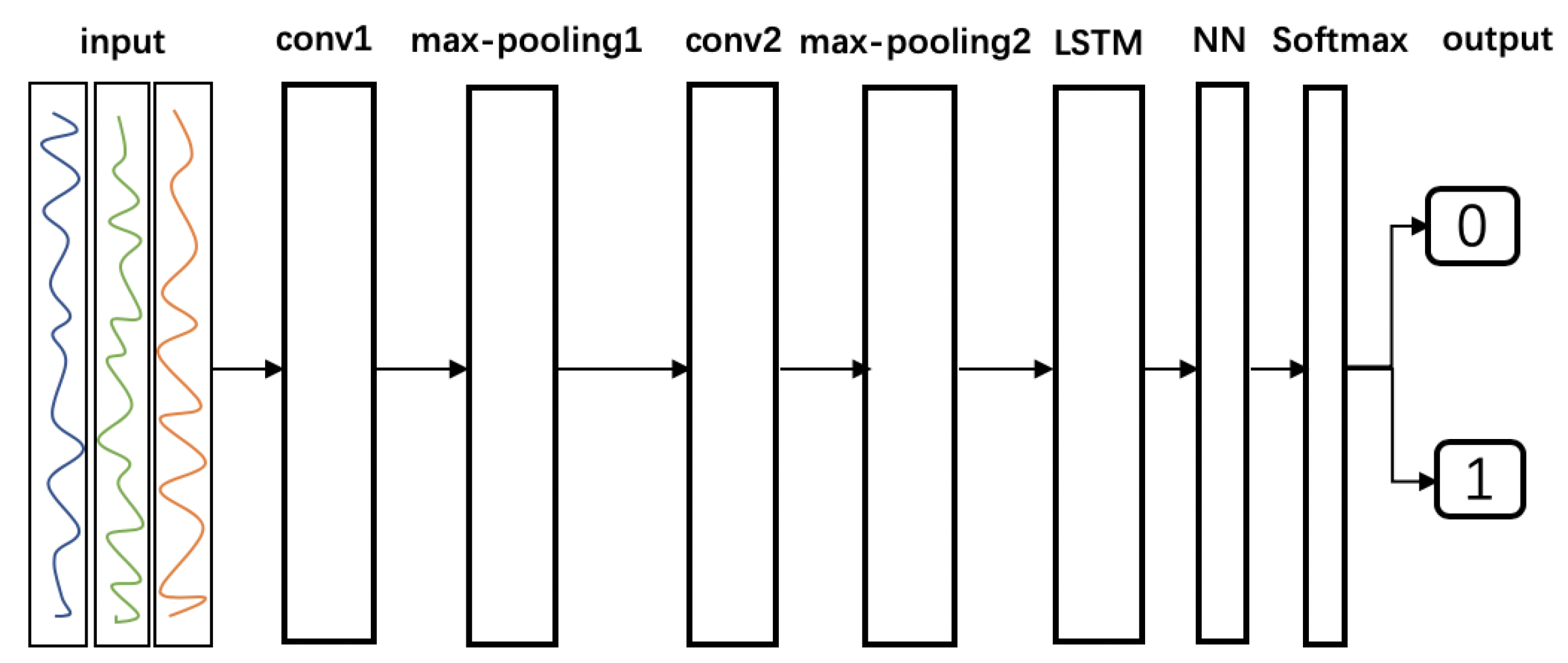
3.2. Neural Network Architecture
The proposed anomaly detection model consists of CNN and LSTM layers connected in a linear structure.
Figure 4 presents the entire network structure. The detector uses the preprocessed data as the input, which is a sequence of data consisting of time-series normal and abnormal data. In the sliding window, CNN layers are used to extract the spatial features. LSTM layers are used to extract the temporal features. Finally, a Softmax classifier and the typical fully connected neural network (NN) layers are linearly connected. Detailed information on each layer is provided in the following.
Convolutional neural networks: Automatic feature-based approaches are the most commonly used methods; they adopt deep-learning models successfully for time-series classification and solving classification problems, particularly convolutional neural networks (CNNs) [
27]. Therefore, a CNN layer is firstly adopted as an automatic feature-based approach for time-series classification. It consists of an input layer, an output layer, and multiple hidden layers. These hidden layers usually consist of convolutional layers, activation function layers, i.e., pooling layers, ReLU, normalization layers, and fully connected layers. The input of a convolutional layer often has three dimensions: weight, height, and the number of channels. The input in the first layer is convolved by
m three-dimensional filters, which are applied at all the input channels.
In our case, the input time series is a sequence of sliding windows mentioned in
Section 1.2:
, The first dimension is the count of the sliding windows
, the second dimension is the sliding window size
E, and the channel size is set to 1.
The output feature map from the first convolutional layer is then given by convolving each filter, which could be denoted as Equation (
4):
where the circledast ⊛ denotes the convolution operation.
is referred to as feature map and
is the filter for the convolutional layer. The dimension of the feature map depends on the step size (stride) for shifting the kernel.
i refers to the feature map index at the second dimension and m refers to the feature map index at the third dimension. Note that the weight matrix only has one channel, because the number of input channels is one in this case. The output is passed through the non-linearity g to ; this is similar to that of the feed-forward neural network.
In each subsequent layer
, the input feature map
, where
z is the size of the output filter map from the previous convolution. Therefore, we obtain the following Equation (
5)
The output is passed to through the non-linear g. Then, the output is fed into a pooling layer, which is generally a max-pooling layer and functions as a subsampling layer. In the proposed model, a deep CNN architecture is formed by ReLU and multiple convolution and pooling layers, which are stacked on top of one another. Furthermore, the output of the last pooling layer is fed as an input into the LSTM networks.
Long short-term memory networks: Before introducing LSTM, we need to introduce RNNs, because LSTM is an improved version of RNN. RNNs are a special architecture of neural networks that can effectively incorporate temporal dependencies within the input data. This can be achieved by unrolling a neural network on the temporal axis, where the network at each time step is provided with feedback connections from the previous time steps. Training a recurrent neural network with gradient descent requires back-propagating gradients through the entire architecture in order to calculate the loss function’s partial derivative while considering each parameter of the model. As the chain rule is applied many times in back-propagation, it becomes challenging to model long-term dependencies within sequences with a large number of time steps. To solve this problem, LSTM networks incorporate gating mechanisms to enable the model to decide whether to accumulate or forget certain information about the transferred cell state. This allows the network to operate at different timescales and, therefore, effectively model short- as well as long-term dependencies. LSTM has been proven to perform well in many recent publications and is rather easy to train for time-series classification [
28]. Therefore, LSTM has become the baseline architecture for tasks where sequential data with temporal information have to be processed.
In our case, multi-layered LSTM RNNs were built. As mentioned in the previous section, the input of the LSTM cell is the output of the last pooling layer of the previous CNNs. Note that dropouts with a certain probability are added to the inputs and outputs of the given cell. Finally, the output of the stacked LSTM cells is then fed into the neural networks with a Softmax classifier.
4. Model Evaluation
4.1. Loss Function
Softmax cross entropy is used to define the loss function in the anomaly detector. In the output layer of the neural network of the proposed anomaly detector, an array
that contains the class scores for each of the training instances is computed.
N is the number of training instances.
C denotes the number of classification labels. For the anomaly detection problem,
, as there are only two labels, “normal” and “abnormal”. The class score
is computed with the Softmax function, as shown in Equation (
6), which is a normalized exponential function taking as the input a vector of
C real numbers; it is normalized into a probability distribution consisting of
C probabilities.
where
is the exponential score of the
ith component of the input vector. After applying Softmax, each component of the input vector occurs in the interval
, and the components add up to 1, so that they can be interpreted as probabilities. The cross-entropy loss is defined as Equation (
7):
where
and
are the ground truth and the predicted score for each class in C. Therefore, the Softmax cross entropy loss can be denoted as Equation (
8):
To avoid the over-fitting issue, regularization techniques are used by penalizing the coefficients. In fact, these techniques penalize the weight matrices of the nodes in deep learning. L1 and L2 are the most common types of regularization. The general cost function is updated by adding another regularization term. The values of the weight matrices decrease after the addition of the regularization term because a neural network with smaller weight matrices often adopts simpler models. Therefore, over-fitting will also be reduced to a considerable extent. In this paper, L2 regularization is adopted; therefore, the final loss function is defined as Equation (
9):
where the term
is simply the squared Euclidean norm of the weight matrix of the hidden layer of the network.
is added to allow us to control the strength of the regularization.
4.2. Performance Evaluation Metrics
A confusion matrix that provides the outcomes of counting detected instances correctly and incorrectly for each type of event could be used to establish the measures of the classification efficiency. As an error metric, a confusion matrix is a specific table layout that can visualize a classifier’s performance in the field of machine learning. When it comes to a binary classification task, the terms “positive” and “negative” are used to reflect the classifier’s prediction, and the terms “true” and “false” are used to reflect whether this prediction is consistent with the external judgment (which is sometimes called “observation”). In view of these definitions, the confusion matrix is formulated and listed in
Table 1.
Accuracy, precision, recall, and F-score are popular performance measures for machine learning models. Equations (
10)–(
13) show their definitions, respectively, on the basis of the confusion matrix shown in
Table 1.
Intuitively, it is not difficult to understand accuracy: the proportion of correctly categorized samples to all the samples should be accurate. In general, higher accuracy is associated with a better classifier. Precision reflects the classifier’s ability to label positive samples and negative samples correctly, and recall reflects the classifier’s ability to identify all the positive samples. The F-score could be denoted by the or measures; it serves as a weighted harmonic mean of precision and recall. An measure reaches its best value at 1 and its worst score at 0. When , and are equivalent, and the recall and the precision are equally important.
5. Experiments
In this section, we mainly introduce the datasets and hyperparameters for the proposed anomaly. The experiments were mainly implemented with Python, the platform of deep learning was mainly based on TensorFlow, and TensorBoard was used as a visualization tool for TensorFlow.
5.1. Benchmark Datasets
The datasets discussed in this section are labeled time-series anomaly detection benchmark datasets provided as a part of the Yahoo Webscope program. These datasets are designed to be benchmark datasets for judging an anomaly detection algorithm; some comparative studies on anomaly detection were successfully conducted on these datasets [
24,
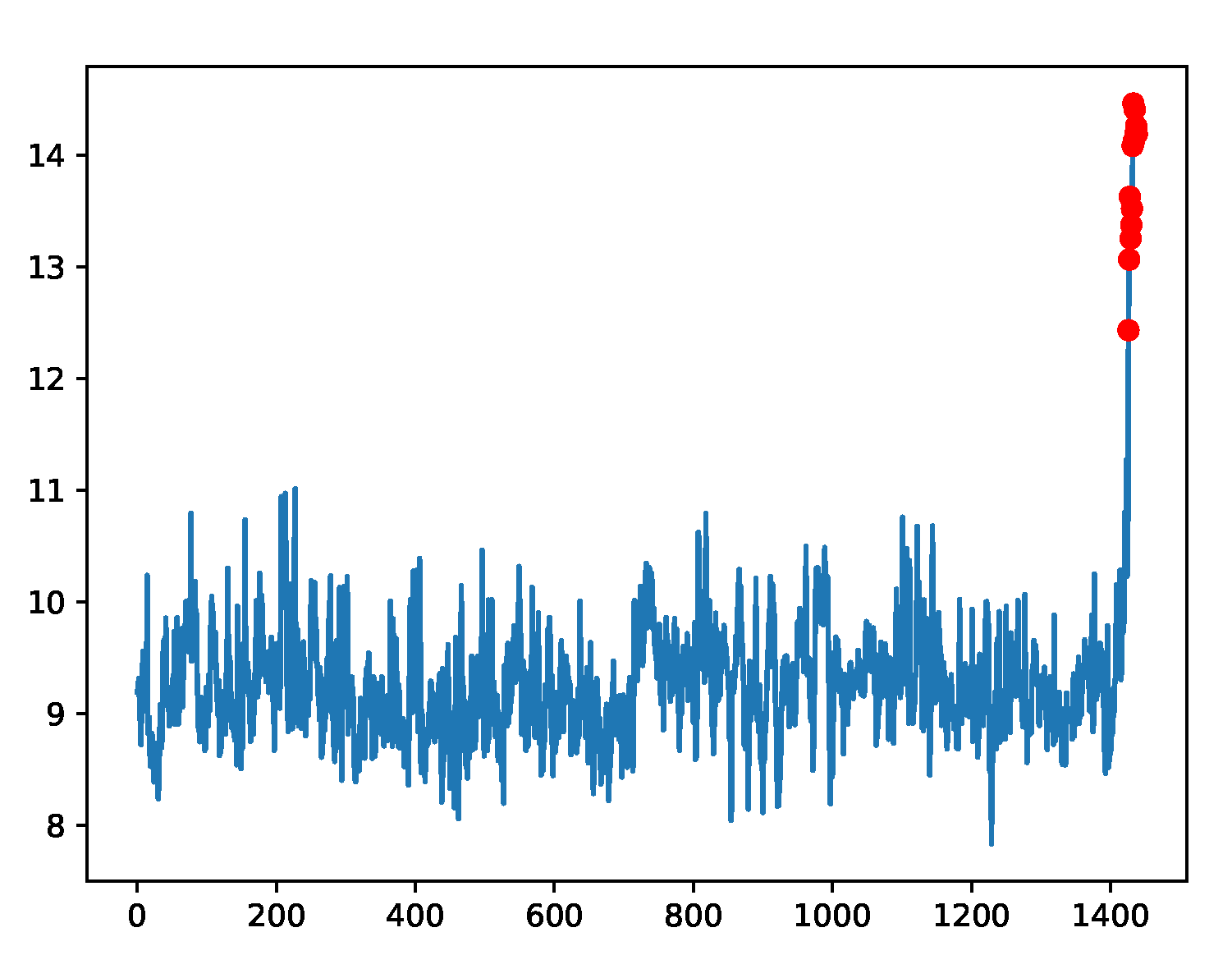
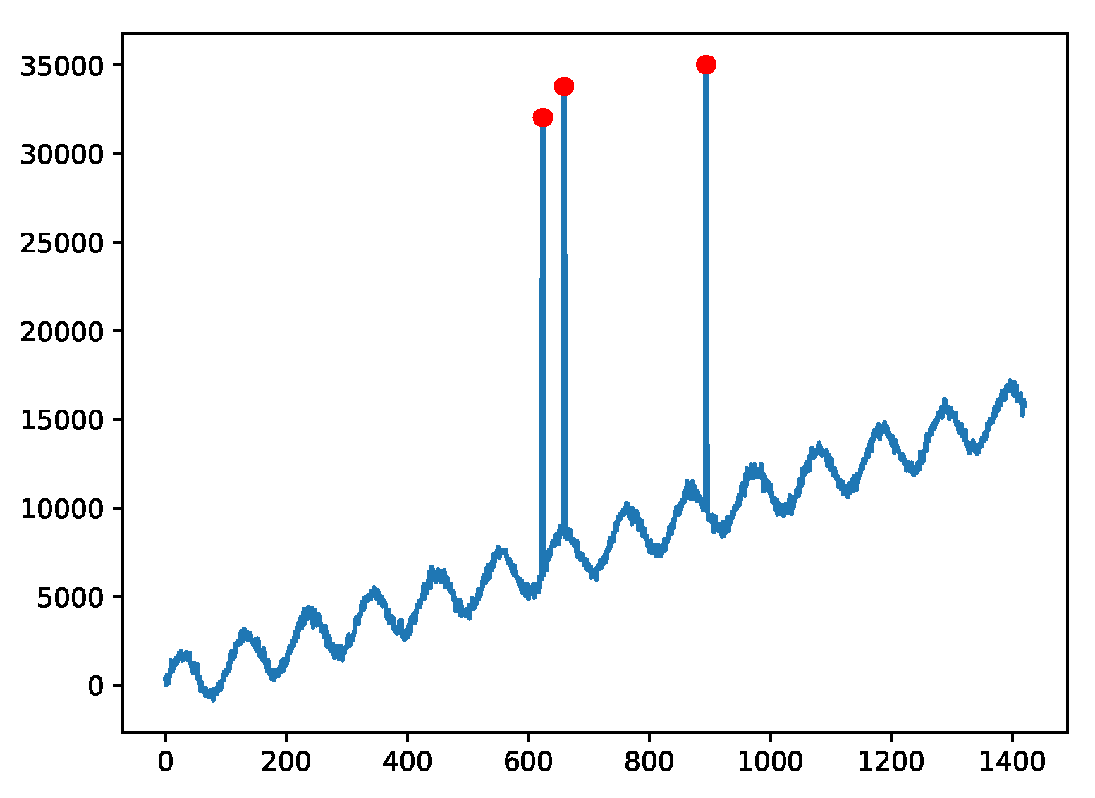
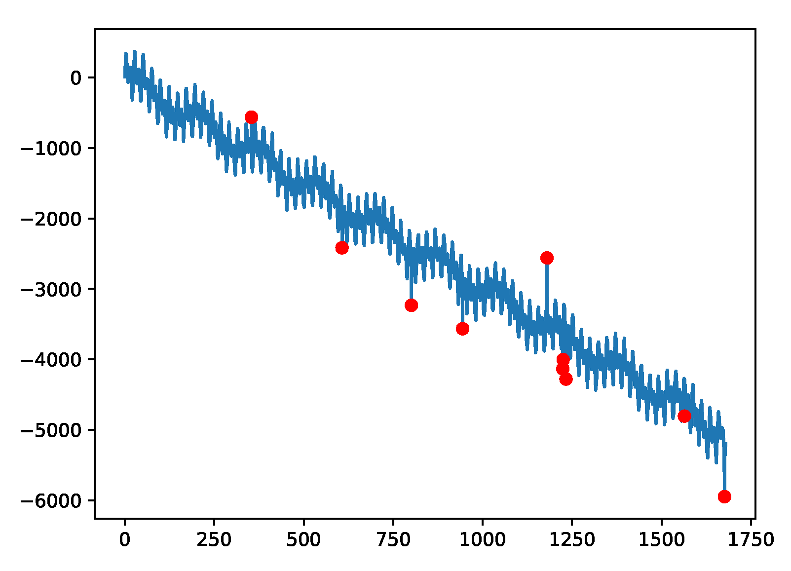
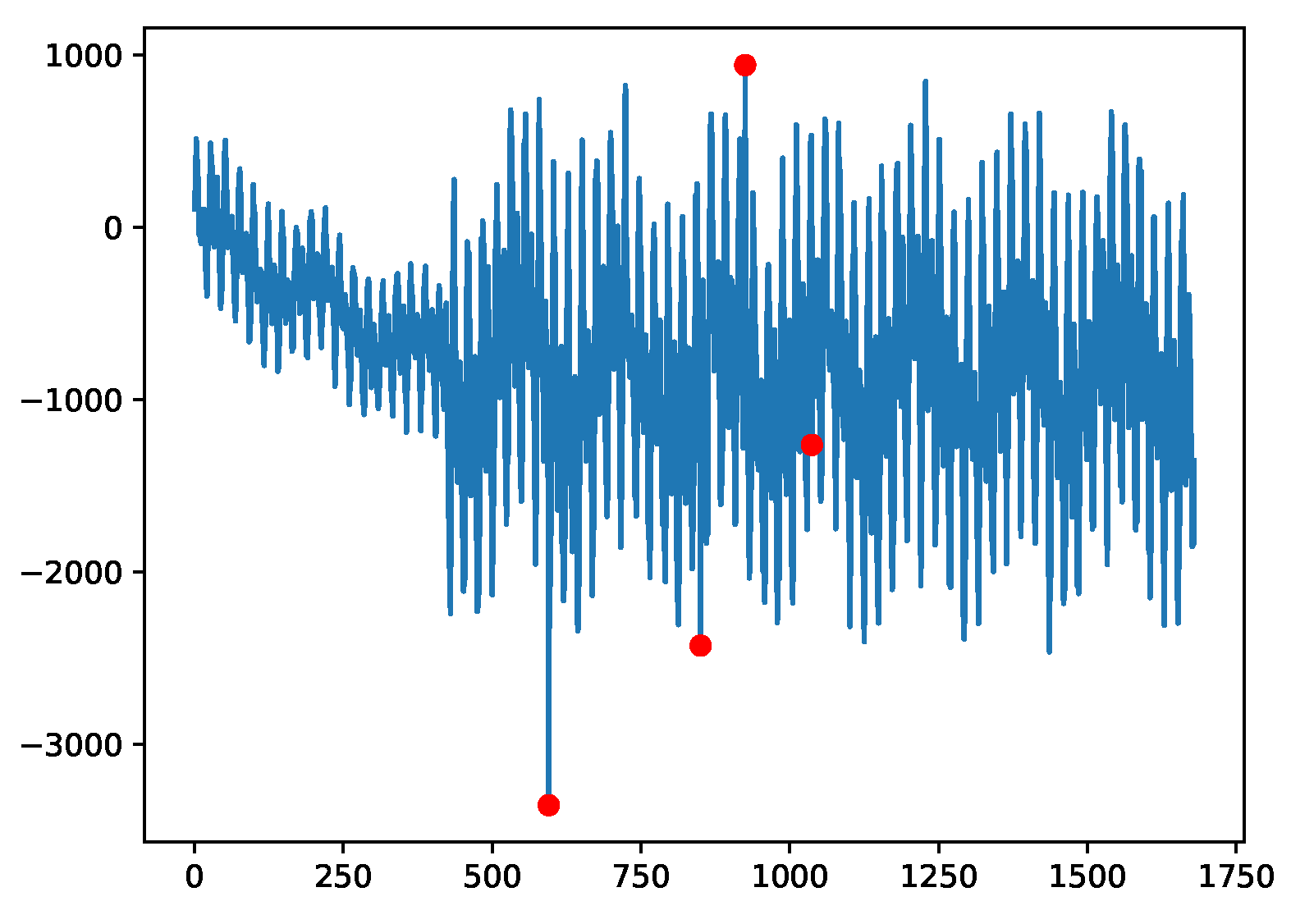
29]. The dataset covers both real and synthetic time series, as well as labeled anomaly points. The dataset can test the accuracy of various types of anomaly detection methods, including outliers and change points. The synthetic dataset includes various time series with different trends, noise, and seasonality. The A1 Benchmark takes the real production traffic to certain Yahoo properties as the basis. The other three benchmarks take the synthetic time series as the basis. The A2 and A3 Benchmarks include outliers, while the A4 Benchmark dataset includes change-point anomalies. The fields in each data file are delimited with (“,”) characters. The time-series samples are shown in
Figure 5,
Figure 6,
Figure 7 and
Figure 8 for the four sub-benchmarks, respectively.
5.2. AIOps KPI Monitoring Datasets
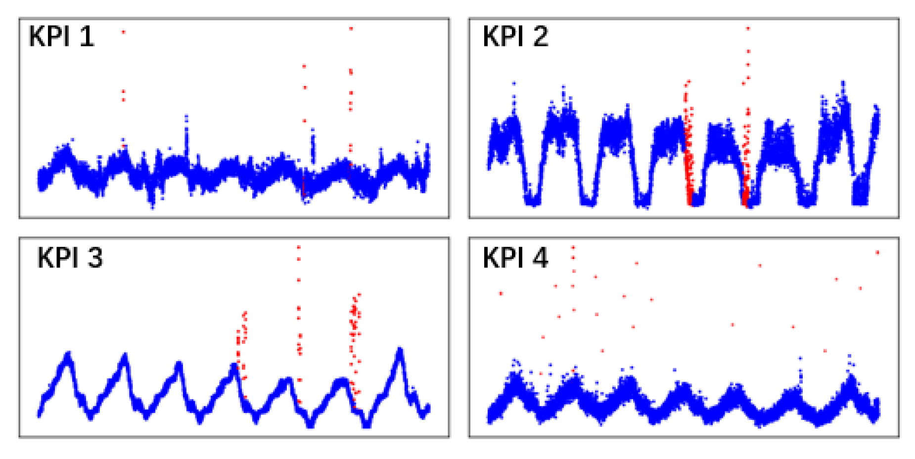
As the anomaly detector presented in this paper seeks to perform anomaly detection in the monitoring of KPIs in a cloud environment, on the one hand, we need to verify the performance of KPI-TSAD through the benchmark datasets. On the other hand, we need to apply the anomaly detector to a KPI monitoring dataset. The datasets discussed in this part were taken from an AIOps Challenge held by Tsinghua University in 2018. According to the organizer’s description, the datasets of this AIOps Challenge are all from the cloud application performance monitoring platform used by many of the large Internet providers in China. We randomly extracted four KPI datasets to verify the proposed anomaly detector. As shown in
Table 2, the ratio of normal samples and abnormal samples in the dataset is obviously very uneven, with abnormal samples representing less than 10% of the total sample.
Figure 9 shows the visualization effects of these four types of KPI data. All types of KPI data show a certain degree of periodicity and trend.
5.3. Hyper-Parameters of the Proposed Anomaly Detector in the experiments
In this subsection, we introduce some common hyperparameters for the proposed detector used in the experiment. As shown in
Table 3, these hyperparameters are consistent in all experiments. In addition, some personalized hyper-parameters vary from dataset to dataset.
Table 4 shows the optimized hyperparameter settings on different datasets.
6. Results and Discussion
We conducted several comparative experiments to demonstrate the effectiveness of the proposed method from different perspectives. On the one hand, we compared the proposed anomaly detection method with the anomaly detection method mentioned in other papers on the same dataset. On the other hand, we compared different oversampling methods that were integrated in KPI-TSAD to illustrate the superiority of VAEGEN oversampling method. Finally, we applied KPI-TSAD to the datasets from real production environments and prove the effectiveness of this method again.
6.1. Comparisons with State-of-The-Art Methods
In this subsection, we evaluate KPI-TSAD on Yahoo’s anomaly detection benchmark datasets.
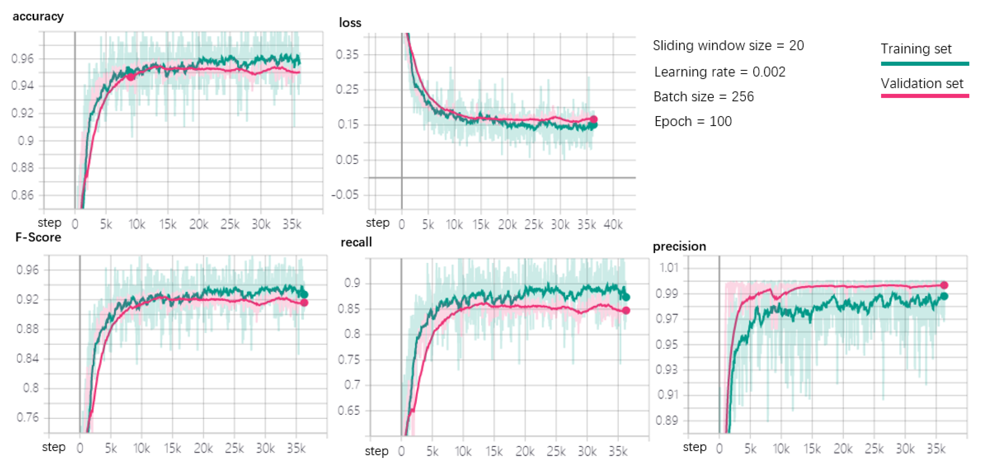
Figure 10 shows that the proposed model performs well on the A1Benchmark dataset wherein the anomalies are taken from a real-world application and manually labeled. The experimental results show the performance of the detector in terms of accuracy, loss, F-score, recall, and precision, respectively. We adopt TensorFlow as our machine learning platform, and TensorBoard is employed to present the experimental results where it can be used as a visualization plug-in of TensorFlow. As shown in the figure, we only add the instructions for various training hyperparameters in the upper right corner of the original dashboard, where the size of sliding window is set to 20, the learning rate is set to 0.002, the batch size is set to 258, and the epoch is 100. As shown in the figure, the total number of steps in the training process for the whole in-depth learning process is 35,000. It can be seen that when the training involves close to 10,000 steps, the values of the relevant evaluation metrics in the model stabilize, with no obvious data fluctuations. At the same time, the loss function reaches the minimum value when the training process takes close to 10,000 steps, and fluctuations in the minimum value also tend to be relatively stable. Finally, the green curve represents the effect of training on the training set, while the pink curve represents its effect on the validation set. From the sub-graphs corresponding to each metric, we can see that the fitting effect on the training set and validation set performs well, as the fitting values between them basically coincide, with no obvious gaps. Finally, it is clear that the model performs very well on the dataset, as both the accuracy and F-score exceed 0.9.
Next, we continue to evaluate the detector on other Yahoo benchmark datasets and conduct a comparison with some of the state-of-the-art methods discussed in
Section 6.1. The Olympic model is used in TMM and EGADS, and the ExtremeLowDensityModel is used in ADM. The default values of all the other parameters are used. Both Twitter’s anomaly detection and EGADS calculate the threshold themselves for each time series. The experiments for Twitter AD and Yahoo EGADS are the same as that in [
24].
Table 5 shows that the proposed method outperforms other existing threshold-based anomaly detection methods. Compared with DeepAnT, which is an unsupervised learning detector, the proposed method also performs better on most datasets.
From the experimental results, we infer that the proposed method is indeed much better than the threshold-based methods and the unsupervised learning detector considered. We can see that the Twitter anomaly detection method based on threhold has poor effect on Yahoo’s dataset, and it could not detect any anomalies on the A2Benchmark dataset, whereas the ExtremeLowDensityModel in Yahoo’s EGADS framework performs poorly, and the overall F-score does not exceed 0.6, DeepAnT is from a recent anomaly detection research. It employs unsupervised learning method for anomaly detection. From the experimental results, we can see that KPI-TSAD performs better than DeepAnt except on the A3Benchmark dataset, and our proposed method reaches the best performance on the A1Benchmark dataset, and the F-Score reaches 0.92.
Finally, we have to emphasize that, from the above comparison, we cannot make conclusions about the value of our method over any other approaches in any scenario. Threshold-based and unsupervised learning-based detectors are relatively simple in terms of application: At the very least, these methods do not require preparing a training set in advance. Only in terms of the performance of anomaly detection is the proposed approach indeed much better than these methods.
6.2. Comparisons with Traditional Oversampling Methods
To highlight the effectiveness of the oversampling model VAE method used in this scheme, we replace the oversampling part of our model with two classical oversampling methods, SMOTE and ADASYN, for a quantitative comparison. All of these experiments were conducted on both the A1Benchmark and the A2Benchmark datasets. It is necessary to emphasize that, during the entire model comparison process, the model parameters of the other parts are the same except for the oversampling method. To improve the validity of the experiment, we performed a comparative experiment on four different datasets. The metrics measured in the experiment are the four classic metrics: accuracy, F-score, recall, and precision. The results can be seen in
Table 6. They imply that the VAE oversampling method used in the proposed detector is considerably better than SMOTE and ADASYN. It can be seen that the scheme of integrating SOMTE and ADASYN is not good on the A1Benchmark dataset; however, the proposed scheme which integrates VAEGEN is very effective, and the F-Score is close to 0.9. On A1Benchmark, the schemes of integrating SMOTE method are also good, its F-Score exceeds 0.9, however, it is still not as good as KPI-TSAD. It is not difficult to see that the performance of KPI-TSAD has outstanding advantages.
6.3. Comparisons with Other Deep Neural Networks
In this section, we seek to verify further whether our current neural network framework is the optimal network structure; therefore, we try to make some adjustments to the network structure and perform experimental verification of anomaly detection. First, we consider the CNN method alone, which includes three convolutional layers and two pooling layers, to extract features from the data automatically, and finally, use Softmax directly. In the second comparison experiment, we use a network layer with two layers of DNN added to the previous CNN method for comparison training. The results of the experimental comparison are shown in
Table 7. The performance metrics used in this experimental comparison are still the four classic evaluation metrics. As shown by the experimental results in
Table 7, the results of KPI-TSAD are superior to those from the other networks.
It shows that more than one deep learning network can be adopted in the training process for an anomaly detector. Different network structures obviously have some differences in the experimental results. From the experimental results, it can be seen that, if only CNN is used as the whole network structure, F-score is close to 0.9, and its effect is close to that of CNN plus DNN. However, when CNN is combined with LSTM, the experimental results are better than the other methods, because this method can extract both spatial and temporal features, which can improve the performance of anomaly detection.
6.4. Performance on Real Production Datasets
Thus far, we have verified the proposed detector on public benchmark datasets. In this subsection, we again apply KPI-TSAD to several real KPI monitoring datasets from an AIOps2018 Challenge held jointly by Tsinghua University and several well-known Internet providers in China. We selected four KPI datasets from these datasets for the anomaly detection experiments, as mentioned in
Section 5.2. The experimental results presented in
Table 8 show that most of the F1 scores of the model are above 0.7, which means that the proposed model can also perform well and that this model can indeed be used in production environments for KPI anomaly detection.
The datasets used in the previous experiments are public datasets for scientific experiments. In this section, we directly apply the proposed anomaly detection method on the KPIs data from real cloud platforms. From the experimental results, we can see that, although the results of the experiment are slightly worse than that of the public datasets, the average F-score is over 0.72. It proves that KPI-TSAD performs well in the production environments and has good generalization capability.
7. Conclusions
In this paper, we propose an anomaly detector KPI-TSAD based on supervised deep learning. We attempt to solve the anomaly detection problem by positioning it as a classification problem. A novel oversampling method VAEGEN is proposed to solve the imbalanced classification problem. Yahoo’s anomaly detection benchmark datasets were used to verify the performance of KPI-TSAD, and the detector performed well on the benchmark datasets. Compared with other popular oversampling approaches, the proposed method VAEGEN also achieved better results. Lastly, we applied KPI-TSAD to four KPI datasets from real production environments; the experimental results show that KPI-TSAD could achieve good results with respect to production.
Although supervised learning-based methods achieve good performance in anomaly detection, we must admit that they have their limitations, as the training set must be prepared before these methods can be used for anomaly detection. Moreover, the process of labeling a high-quality training set is very labor-intensive, which poses a particular obstacle to the application of anomaly detectors. Therefore, in the future, we will further explore an unsupervised anomaly detection method based on some of the ideas presented in this paper.
Finally, the research in this paper mainly focuses on the anomaly detection for single KPI, as the data used for training come from the same kind of KPI. However, the anomaly detector for multiple KPIs is more useful in the production environment. We will also start the research on this part based on the research of this paper.
Author Contributions
Conceptualization, J.Q. and C.Q.; methodology, J.Q.; experiment, J.Q. and C.Q.; manuscript review and modifications suggestion, Q.D.
Funding
This work was supported by the National Natural Science Foundation of China (Grant No. 61672384).
Acknowledgments
We have to acknowledge the OPNFV project from Linux open source foundation, because some of the ideas come from the OPNFV community. We have obtained lots of inspiration and discussion. We give thanks to the public datasets provided by the Yahoo and AIOps Challenges; those datasets provided strong support for our experiments. Finally, the authors are grateful for the comments and reviews from the reviewers and editors.
Conflicts of Interest
The authors declare no conflict of interest.
References
- Assendorp, J.P. Deep Learning for Anomaly Detection in Multivariate Time Series Data. Ph.D. Thesis, Hochschule für Angewandte Wissenschaften Hamburg, Hamburg, Germany, 2017; pp. 9–32. [Google Scholar]
- Kingma, D.P.; Welling, M. Auto-encoding variational bayes. arXiv 2013, arXiv:1312.6114. [Google Scholar]
- Chen, Y.; Mahajan, R.; Sridharan, B.; Zhang, Z.L. A provider-side view of web search response time. ACM SIGCOMM Comput. Commun. Rev. 2013, 43, 243–254. [Google Scholar] [CrossRef]
- Knorn, F.; Leith, D.J. Adaptive kalman filtering for anomaly detection in software appliances. In Proceedings of the IEEE INFOCOM Workshops, Phoenix, AZ, USA, 13–18 April 2008; pp. 1–6. [Google Scholar]
- Lee, S.B.; Pei, D.; Hajiaghayi, M.; Pefkianakis, I.; Lu, S.; Yan, H.; Ge, Z.; Yates, J.; Kosseifi, M. Threshold compression for 3g scalable monitoring. In Proceedings of the IEEE INFOCOM, Orlando, FL, USA, 25–30 March 2012; pp. 1350–1358. [Google Scholar]
- Yan, H.; Flavel, A.; Ge, Z.; Gerber, A.; Massey, D.; Papadopoulos, C.; Shah, H.; Yates, J. Argus. End-to-end service anomaly detection and localization from an ISP’s point of view. In Proceedings of the IEEE INFOCOM, Orlando, FL, USA, 25–30 March 2012; pp. 2756–2760. [Google Scholar]
- Liu, D.; Zhao, Y.; Xu, H.; Sun, Y.; Pei, D.; Luo, J.; Jing, X.; Feng, M. Opprentice: Towards practical and automatic anomaly detection through machine learning. In Proceedings of the 2015 ACM Measurement Conference, Tokyo, Japan, 28–30 October 2015; pp. 211–224. [Google Scholar]
- Laptev, N.; Amizadeh, S.; Flint, I. Generic and scalable framework for automated time-series anomaly detection. In Proceedings of the 21th ACM SIGKDD Knowledge Discovery and Data Mining, Sydney, NSW, Australia, 10–13 August 2015; pp. 1939–1947. [Google Scholar]
- Vallis, O.; Hochenbaum, J.; Kejariwal, A. A novel technique for long-term anomaly detection in the cloud. In Proceedings of the 6th USENIX Workshop on Hot Topics in Cloud Computing, Philadelphia, PA, USA, 17–18 June 2014. [Google Scholar]
- Li, J.; Pedrycz, W.; Jamal, I. Multivariate time series anomaly detection: A framework of Hidden Markov Models. Appl. Soft Comput. 2017, 60, 229–240. [Google Scholar] [CrossRef]
- Lin, Q.; Hammerschmidt, C.; Pellegrino, G.; Verwer, S. Short-term time series forecasting with regression automata. In Proceedings of the KDD ‘16, San Francisco, CA, USA, 13–17 August 2016. [Google Scholar]
- Görnitz, N.; Braun, M.; Kloft, M. Hidden markov anomaly detection. In Proceedings of the International Conference on Machine Learning, Lille, France, 6–11 July 2015; pp. 1833–1842. [Google Scholar]
- Liu, X.; Lin, Q.; Verwer, S.; Jarnikov, D. Anomaly Detection in a Digital Video Broadcasting System Using Timed Automata. arXiv 2017, arXiv:1705.09650. [Google Scholar]
- Kwon, D.; Kim, H.; Kim, J.; Suh, S.C.; Kim, I.; Kim, K.J. A survey of deep learning-based network anomaly detection. Cluster Comput. 2019, 22, 949–961. [Google Scholar] [CrossRef]
- Ibidunmoye, O.; Hernández-Rodriguez, F.; Elmroth, E. Performance anomaly detection and bottleneck identification. ACM Comput. Surv. (CSUR) 2015, 48, 4. [Google Scholar] [CrossRef]
- Agrawal, S.; Jitendra, A. Survey on anomaly detection using data mining techniques. Procedia Comput. Sci. 2015, 60, 708–713. [Google Scholar] [CrossRef]
- Chandola, V.; Banerjee, A.; Kumar, V. Anomaly detection: A survey. ACM Comput. Surv. (CSUR) 2009, 41, 15. [Google Scholar] [CrossRef]
- Amer, M.; Goldstein, M.; Abdennadher, S. Enhancing one-class support vector machines for unsupervised anomaly detection. In Proceedings of the ACM SIGKDD Workshop on Outlier Detection and Description, Chicago, IL, USA, 11 August 2013; pp. 8–15. [Google Scholar]
- Erfani, S.M.; Rajasegarar, S.; Karunasekera, S.; Leckie, C. High-dimensional and large-scale anomaly detection using a linear one-class SVM with deep learning. Pattern Recognit. 2016, 58, 121–134. [Google Scholar] [CrossRef]
- Nicolau, M.; McDermott, J. One-class classification for anomaly detection with kernel density estimation and genetic programming. In Proceedings of the European Conference on Genetic Programming, Porto, Portugal, 30 March–1 April 2016; pp. 3–18. [Google Scholar]
- An, J.; Cho, S. Variational autoencoder based anomaly detection using reconstruction probability. Spec. Lect. IE 2015, 2, 1–18. [Google Scholar]
- Sölch, M.; Bayer, J.; Ludersdorfer, M.; van der Smagt, P. Variational inference for on-line anomaly detection in high-dimensional time series. arXiv 2016, arXiv:1602.07109. [Google Scholar]
- Ordonez, F.; Roggen, D. Deep convolutional and lstm recurrent neural networks for multimodal wearable activity recognition. Sensors 2016, 16, 115. [Google Scholar] [CrossRef] [PubMed]
- Munir, M.; Siddiqui, S.A.; Dengel, A.; Ahmed, S. DeepAnT: A Deep Learning Approach for Unsupervised Anomaly Detection in Time Series. IEEE Access 2019, 7, 1991–2005. [Google Scholar] [CrossRef]
- Kejariwal, A. Introducing Practical and Robust Anomaly Detection in a Time Series. 2015. Available online: https://blog.twitter.com/ (accessed on 21 August 2019).
- Abdi, L.; Hashemi, S. To combat multi-class imbalanced problems by means of over-sampling techniques. IEEE Trans. Knowl. Data Eng. 2015, 28, 238–251. [Google Scholar] [CrossRef]
- Zhao, B.; Lu, H.; Chen, S.; Liu, J.; Wu, D. Convolutional neural networks for time series classification. J. Syst. Eng. Electron. 2017, 28, 162–169. [Google Scholar] [CrossRef]
- Karim, F.; Majumdar, S.; Darabi, H.; Chen, S. LSTM fully convolutional networks for time series classification. IEEE Access 2017, 6, 1662–1669. [Google Scholar] [CrossRef]
- Thill, M.; Konen, W.; Bäck, T. Online anomaly detection on the webscope S5 dataset: A comparative study. In Proceedings of the Evolving and Adaptive Intelligent Systems (EAIS), Ljubljana, Slovenia, 31 May–2 June 2017; pp. 1–8. [Google Scholar]
Figure 1.
Anomaly detector role in APM platform.
Figure 1.
Anomaly detector role in APM platform.
Figure 2.
The entire workflow of the proposed detector (the grey part in the figure represents the distribution of abnormal samples.).
Figure 2.
The entire workflow of the proposed detector (the grey part in the figure represents the distribution of abnormal samples.).
Figure 3.
Structure of variational auto-encoder.
Figure 3.
Structure of variational auto-encoder.
Figure 4.
Structure of the neural networks for KPI-TSAD.
Figure 4.
Structure of the neural networks for KPI-TSAD.
Figure 5.
Example plot for the A1 data, which were taken from real world applications and anomalies were manually labeled as red marks.
Figure 5.
Example plot for the A1 data, which were taken from real world applications and anomalies were manually labeled as red marks.
Figure 6.
Example plot for the A2 data which were generated synthetically with a trend, a seasonal (periodic) component and noise; anomalies were added at random instances.
Figure 6.
Example plot for the A2 data which were generated synthetically with a trend, a seasonal (periodic) component and noise; anomalies were added at random instances.
Figure 7.
Example plot for the A3 data, which were generated synthetically with a trend, three seasonal (periodic) components and noise; anomalies were added at random instances.
Figure 7.
Example plot for the A3 data, which were generated synthetically with a trend, three seasonal (periodic) components and noise; anomalies were added at random instances.
Figure 8.
Example plot for the A4 data; change point anomalies are introduced.
Figure 8.
Example plot for the A4 data; change point anomalies are introduced.
Figure 9.
Four KPIs from real production environments.
Figure 9.
Four KPIs from real production environments.
Figure 10.
Anomaly detection performance for A1Benchmark.
Figure 10.
Anomaly detection performance for A1Benchmark.
Table 1.
Confusion matrix.
Table 1.
Confusion matrix.
| | Positive | Negative |
|---|
| True | (TP)
a real anomaly point,
be predicted correctly | (TN)
a real normal point,
be predicted correctly |
| False | (FP)
a real anomaly point,
NOT be predicted correctly | (FN)
a real normal point,
NOT be predicted correctly |
Table 2.
Description of the four KPIs monitoring datasets.
Table 2.
Description of the four KPIs monitoring datasets.
| | KPI 1 | KPI 2 | KPI 3 | KPI3 |
|---|
| Total points | 128,562 | 128,853 | 129,128 | 129,035 |
Anomaly points
(ratio) | 10,550
(8.21%) | 9581
(7.44%) | 7863
(6.09%) | 7666
(5.94%) |
| Duration | 91 days | 91 days | 91 days | 91 days |
Sample Frequency
(point/day) | 1412.77 | 1415.97 | 1418.99 | 1417.97 |
Table 3.
Hyperparameters of the neural networks.
Table 3.
Hyperparameters of the neural networks.
| Type | Parameters |
|---|
| convolution | Filter = [4,1,1,64] |
| activation | ReLU |
| max-pooling | Kernel Size = [1,2,1,1]
strides = [1,2,1,1]
padding = ‘SAME’ |
| convolution | Filter = [4,1,64,64] |
| activation | ReLU |
| max-pooling | Kernel Size = [1,2,1,1]
strides = [1,2,1,1]
padding = ‘SAME’ |
| convolution | Filter = [4,1,64,64] |
| LSTM | Input size = 64 |
| Dense | Input size = 2 |
| Softmax | loss function = cross entropy |
Table 4.
Key hyperparameters of the proposed anomaly detector.
Table 4.
Key hyperparameters of the proposed anomaly detector.
| Type | Window Size | Learning Rate | Batch Size |
|---|
| A1Benchmark | 20 | 0.0002 | 256 |
| A2Benchmark | 12 | 0.0001 | 256 |
| A3Benchmark | 12 | 0.0001 | 128 |
| A4Benchmark | 16 | 0.0001 | 128 |
| AIOps-Dataset | 12 | 0.0002 | 256 |
Table 5.
Comparison with state-of-art anomaly detection methods.
Table 5.
Comparison with state-of-art anomaly detection methods.
| | A1 | A2 | A3 | A4 |
|---|
| Yahoo EGADS | 0.47 | 0.58 | 0.48 | 0.29 |
Twitter AD
Alpha = 0.05 | 0.48 | 0 | 0.26 | 0.31 |
Twitter AD
Alpha = 0.1 | 0.48 | 0 | 0.27 | 0.33 |
Twitter AD
Alpha = 0.2 | 0.47 | 0 | 0.30 | 0.34 |
| DeepAnT | 0.46 | 0.94 | 0.87 | 0.68 |
| Ours | 0.92 | 0.97 | 0.72 | 0.76 |
Table 6.
Performance comparison with other oversampling methods.
Table 6.
Performance comparison with other oversampling methods.
| Datasets | Measure | VAEGEN | SMOTE | ADASYN |
|---|
| A1Benchmark | Accuracy | 0.95 | 0.62 | 0.61 |
| F-Score | 0.92 | 0.54 | 0.56 |
| Precision | 0.99 | 0.72 | 067 |
| Recall | 0.86 | 0.49 | 0.55 |
| A2Benchmark | Accuracy | 0.96 | 0.95 | 0.77 |
| F-Score | 0.97 | 0.94 | 0.79 |
| Precision | 0.99 | 0.99 | 0.98 |
| Recall | 0.93 | 0.91 | 0.66 |
Table 7.
Performance comparison with other deep learning models.
Table 7.
Performance comparison with other deep learning models.
| | Precision | Recall | F-Score | Accuracy |
|---|
| KPI-TSAD | 0.95 | 0.92 | 0.99 | 0.86 |
| CNN + DNN | 0.90 | 0.93 | 0.89 | 0.82 |
| CNN | 0.89 | 0.91 | 0.84 | 0.80 |
Table 8.
Anomaly detection performance for the four KPIs.
Table 8.
Anomaly detection performance for the four KPIs.
| | Accracy | F-Score | Recall | Precision |
|---|
| KPI 1 | 0.77 | 0.72 | 0.79 | 0.80 |
| KPI 2 | 0.75 | 0.74 | 0.83 | 0.78 |
| KPI 3 | 0.83 | 0.68 | 0.81 | 0.77 |
| KPI 4 | 0.85 | 0.77 | 0.91 | 0.73 |
© 2019 by the authors. Licensee MDPI, Basel, Switzerland. This article is an open access article distributed under the terms and conditions of the Creative Commons Attribution (CC BY) license (http://creativecommons.org/licenses/by/4.0/).


