Nondifferentiable G-Mond–Weir Type Multiobjective Symmetric Fractional Problem and Their Duality Theorems under Generalized Assumptions

Abstract

In this article, a pair of nondifferentiable second-order symmetric fractional primal-dual model (G-Mond–Weir type model) in vector optimization problem is formulated over arbitrary cones. In addition, we construct a nontrivial numerical example, which helps to understand the existence of such type of functions. Finally, we prove weak, strong and converse duality theorems under aforesaid assumptions.

1. Introduction

In multiobjective programming problems, convexity plays an important role in deriving optimality conditions and duality results. To relax convexity assumptions involved in sufficient optimality conditions and duality theorems, various generalized convexity notions have been proposed. Multiobjective type programming problem [1] is common in mathematical modeling of realistic phenomenon with a wide spectrum of utilization. Symmetric duality in nonlinear programming deals with the situation where dual of the dual is primal. Special dual problems of optimization are applied to many types of optimization problems. They are used for the proof of optimality of solutions, for designing and a theoretical justification of optimization algorithms, and for physical or economic interpretation of received solutions. Quite often dual problems introduce new meaning to modeled problems. For many interesting applications and developments of multiobjective optimization, we refer to the work of A. Chinchuluun and P.M. Pardalos [2] and the references cited therein.

In economics, we often come across a case where we have to maximize the efficiency of an economic system resulting optimization problems whose objective function is a ratio. Mangasarian [3] proposed the idea of second-order duality for nonlinear optimization problems. The perusal of second-order duality is important due to the computer simulation benefit over the first-order duality since this one supplies narrow ranges for the cost of the objectives when estimations are applied. Suneja et al. [1] and Kim et al. [4] extended the concept of symmetric duality to arbitrary cones.

Suneja et al. [5] considered a pair of multiobjective second order symmetric dual problems of Mond–Weir type without non-negativity constraints and established duality results under $\eta$-bonvexity and $\eta$-pseudobonvexity assumptions. Later, Khurana [6] defined cone-pseudoinvex and strongly cone-pseudoinvex functions and proved duality theorems for a pair of Mond–Weir type symmetric dual multiobjective programs over arbitrary cones. For more information on fractional programming, readers are advised to see [7,8,9,10,11,12,13].

The purpose of the present work is to study second order multiobjective fractional symmetric duality over arbitrary cones for nondifferentiable G-Mond–Weir type program under $G_f$-bonvexity/$G_f$-pseudobonvexity assumptions. The paper is organized as follows. In Section 2, we present some relevant preliminaries. In Section 3, we consider a pair of G-Mond–Weir type nondifferentiable multiobjective second order fractional symmetric dual problems with cone constraints and establish appropriate duality theorems under aforesaid assumptions followed by conclusions.

2. Preliminaries and Definitions

Throughout this paper, $R^n$ stands for the n-dimensional Euclidean space and $R_{+}^n$ for its non-negative orthant. Consider the following vector minimization problem:

(MP)    Minimize $f(x)={\left\{f_1(x),f_2(x),f_3(x),\dots ,f_k(x)\right\}}^T$

    Subject to $X^0=\{x\in X\subset R^n:g_j(x)\le 0,j=1,2,\dots ,m\}$

where $f=\{f_1,f_2,\dots ,f_k\}:X\to R^k$ and $g=\{g_1,g_2,\dots ,g_m\}:X\to R^m$ are differentiable functions defined on $X.$

Definition 1.

A point $\overline{x}\in X^0$ is said to be an efficient solution of (MP) if there exists no other $x\in X^0$ such that $f_r(x)<f_r(\overline{x}),$ for some $r=1,2,\dots ,k$ and $f_i(x)\le f_i(\overline{x}),$ for all $i=1,2,\dots ,k.$

Definition 2.

The positive polar cone $S^{*}$ of a cone $S\subseteq R^s$ is defined by

$$S^{*}=\{y\in R^s:x^{T}y\ge 0,forallx\in S\}.$$

Let $C_1\subseteq R^n$ and $C_2\subseteq R^m$ be closed convex cones with non-empty interiors and $S_1$ and $S_2$ be non-empty open sets in $R^n$ and $R^m$, respectively, such that $C_1\times C_2\subseteq S_1\times S_2$. Suppose $f=(f_1,f_2,\dots ,f_k):S_1\times S_2\to R^k$ is a vector- valued differentiable function.

Definition 3.

The function f is said to be invex at $u\in S_1$ (with respect to $\eta ,$ where $\eta :S_1\times S_2\to R^n$), if $\forall x\in S_1$ and for fixed $v\in S_2$, we have

$$f_i(x,v)-f_i(u,v)\ge {\eta }^T(x,u){\nabla }_x{f}_i(u,v),foralli=1,2,\dots ,k,$$

If the above inequality sign changes to ≤, then f is called incave at $u\in S_1$ with respect to $\eta .$

Definition 4.

The function f is said to be pseudoinvex at $u\in S_1$ (with respect to $\eta ,$ where $\eta :S_1\times S_2\to R^n$), if $\forall x\in S_1$ and for fixed $v\in S_2$, we have

$$\begin{array}{c}\hfill {\eta }^T(x,u){\nabla }_x{f}_i(u,v)\ge 0\Rightarrow f_i(x,v)-f_i(u,v)\ge 0,foralli=1,2,\dots ,k.\end{array}$$

If the above inequality sign changes to $\le ,$ then f is called pseudoincave at $u\in X$ with respect to $\eta .$

Definition 5.

The function f is said to be $G_f$-invex at $u\in S_1$ (with respect to η), if there exists a differentiable function $G_f=(G_{f_1},G_{f_2},\dots ,G_{f_k}):R\to R^k$ such that each component $G_{f_i}:I_{f_i}(S_1\times S_2)\to R$, where $I_{f_i}(S_1\times S_2),i=1,2,3,\dots ,k$ is the range of $f_i$, is strictly increasing on its domain and $\eta :S_1\times S_2\to R^n$, so that $\forall x\in S_1$, for fixed $v\in S_2,$ we have

$$G_{f_i}(f_i(x,v))-G_{f_i}(f_i(u,v))\ge {\eta }^T(x,u)G_{f_i}^{\prime }(f_i(u,v)){\nabla }_x{f}_i(u,v),foralli=1,2,\dots ,k,$$

If the above inequality sign changes to ≤, then f is called $G_f$-incave at $u\in S_1$ with respect to $\eta .$

Definition 6.

The function f is said to be $G_f$-pseudoinvex at $u\in S_1$ (with respect to η), if there exists a differentiable function $G_f=(G_{f_1},G_{f_2},\dots ,G_{f_k}):R\to R^k$ such that each component $G_{f_i}:I_{f_i}(S_1\times S_2)\to R$, where $I_{f_i}(S_1\times S_2),i=1,2,3,\dots ,k$ is the range of $f_i$, is strictly increasing on its domain and $\eta :S_1\times S_2\to R^n$, so that $\forall x\in S_1$, for fixed $v\in S_2,$ we have

$$\begin{array}{c}\hfill {\eta }^T(x,u)G_{f_i}^{\prime }(f_i(u,v)){\nabla }_x{f}_i(u,v)\ge 0\Rightarrow G_{f_i}(f_i(x,v))-G_{f_i}(f_i(u,v))\ge 0,foralli=1,2,\dots ,k.\end{array}$$

If the above inequality sign changes to $\le ,$ then f is called $G_f$-pseudoincave at $u\in X$ with respect to $\eta .$

Definition 7.

The function f is said to be $G_f$-bonvex at $u\in S_1$ (with respect to η), if there exists a differentiable function $G_f=(G_{f_1},G_{f_2},\dots ,G_{f_k}):R\to R^k$ such that each component $G_{f_i}:I_{f_i}(S_1\times S_2)\to R$, where $I_{f_i}(S_1\times S_2),i=1,2,3,\dots ,k$ is the range of $f_i$, is strictly increasing on its domain and $\eta :S_1\times S_2\to R^n$, so that $\forall x\in S_1$, for fixed $v\in S_2$ and $p_i\in R^n,$ we have

$G_{f_i}(f_i(x,v))-G_{f_i}(f_i(u,v))\ge {\eta }^T(x,u)[G_{f_i}^{\prime }(f_i(u,v)){\nabla }_x{f}_i(u,v)+\{G_{f_i}^{″}(f_i(u,v)){\nabla }_x{f}_i(u,v){({\nabla }_x{f}_i(u,v))}^T$

${\displaystyle +G_{f_i}^{\prime }(f_i(u,v)){\nabla }_x{f}_i(u,v)\}{p}_i]-\frac{1}{2}{p}_i^T[G_{f_i}^{″}(f_i(u,v)){\nabla }_x{f}_i(u,v){({\nabla }_x{f}_i(u,v))}^T}$

$$\begin{array}{c}\hfill +G_{f_i}^{\prime }(f_i(u,v)){\nabla }_x{f}_i(u,v)]p_i,foralli=1,2,\dots ,k.\end{array}$$

If the above inequality sign changes to $\le ,$ then f is called $G_f$-boncave at $u\in S_1$ with respect to $\eta .$

Definition 8.

The function f is said to be $G_f$-pseudobonvex at $u\in S_1$ (with respect to η), if there exists a differentiable function $G_f=(G_{f_1},G_{f_2},\dots ,G_{f_k}):R\to R^k$ such that each component $G_{f_i}:I_{f_i}(S_1\times S_2)\to R$, where $I_{f_i}(S_1\times S_2),i=1,2,3,\dots ,k$ is the range of $f_i$, is strictly increasing on its domain and $\eta :S_1\times S_2\to R^n$, so that $\forall x\in S_1$, for fixed $v\in S_2$ and $p_i\in R^n,$ ${\eta }^T(x,u)[G_{f_i}^{\prime }(f_i(u,v)){\nabla }_x{f}_i(u,v)+\{G_{f_i}^{″}(f_i(u,v)){\nabla }_x{f}_i(u,v){({\nabla }_x{f}_i(u,v))}^T+G_{f_i}^{\prime }(f_i(u,v))$

${\displaystyle {\nabla }_{xx}{f}_i(u,v)\}{p}_i]\ge 0\Rightarrow G_{f_i}(f_i(x,v))-G_{f_i}(f_i(u,v))+\frac{1}{2}{p}_i^T[G_{f_i}^{″}(f_i(u,v)){\nabla }_x{f}_i(u,v){({\nabla }_x{f}_i(u,v))}^T}$

$$\begin{array}{c}\hfill +G_{f_i}^{\prime }(f_i(u,v)){\nabla }_{xx}{f}_i(u,v)]p_i\ge 0,foralli=1,2,\dots ,k.\end{array}$$

If the above inequality sign changes to $\le ,$ then f is called $G_f$-pseudoboncave at $u\in S_1$ with respect to $\eta .$

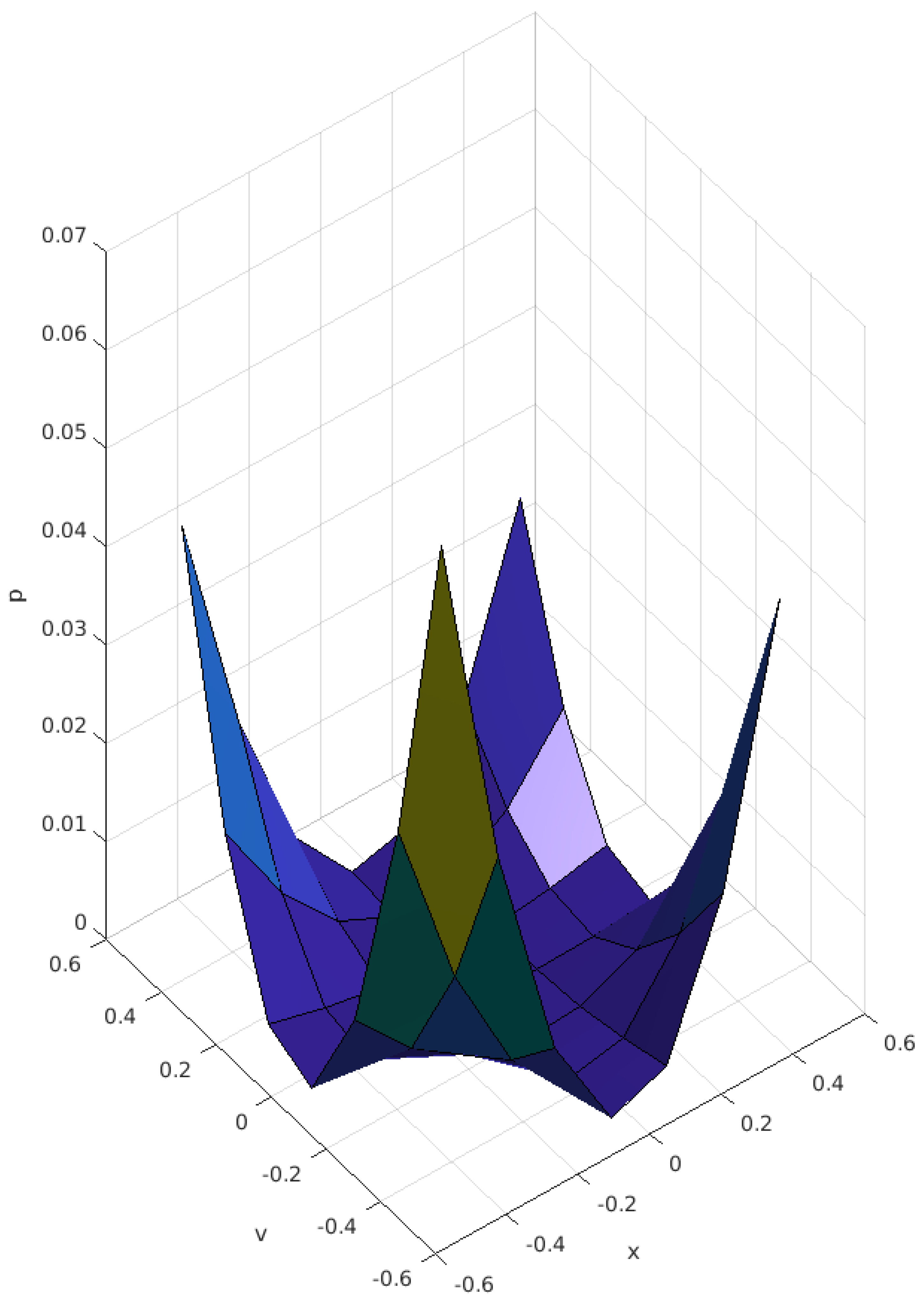
We now give an example of $G_f$-bonvexity with respect to $\eta ,$ but not $\eta$-bonvex.

Example 1.

Let ${\displaystyle k=4,n=1,S_1=S_2=\left[-\frac{\pi }{6},\frac{\pi }{6}\right],C_1=C_2=\left[\frac{-\pi }{6},\frac{\pi }{6}\right]}$.

Let ${\displaystyle f:\left[-\frac{\pi }{6},\frac{\pi }{6}\right]\times \left[-\frac{\pi }{6},\frac{\pi }{6}\right]\to R^4}$ be defined as

$$f(x,y)=\{f_1(x,y),f_2(x,y),f_3(x,y),f_4(x,y)\},$$

where $f_1(x,y)=e^y,f_2(x,y)=x{e}^y,f_3(x,y)=x^{2}si{n}^{2}y,f_4(x,y)=y^2$ and $G_f=\{G_{f_1},G_{f_2},G_{f_3},G_{f_4}\}:R\to R^4$ be defined as:

$$G_{f_1}(t)=t,G_{f_2}(t)=t^4,G_{f_3}(t)=t,G_{f_4}(t)=t^2.$$

Let ${\displaystyle \eta :\left[-\frac{\pi }{6},\frac{\pi }{6}\right]\times \left[-\frac{\pi }{6},\frac{\pi }{6}\right]\to R}$ be given as:

$${\displaystyle \eta (x,u)=xu.}$$

To show that f is $G_f$-bonvex at $u=0$ with respect to $\eta$, we have to claim that

${\pi }_i=G_{f_i}(f_i(x,v))-G_{f_i}(f_i(u,v))-{\eta }^T(x,u)[G_{f_i}^{\prime }(f_i(u,v)){\nabla }_x{f}_i(u,v)+\{G_{f_i}^{″}(f_i(u,v)){\nabla }_x{f}_i(u,v)$

${\displaystyle {({\nabla }_x{f}_i(u,v))}^T\}+G_{f_i}^{\prime }(f_i(u,v)){\nabla }_{xx}{f}_i(u,v)\}{p}_i+\frac{1}{2}{p}_i^T[G_{f_i}^{″}(f_i(u,v)){\nabla }_x{f}_i(u,v)}$

$$\begin{array}{c}\hfill {({\nabla }_x{f}_i(u,v))}^T+G_{f_i}^{\prime }(f_i(u,v)){\nabla }_{xx}{f}_i(u,v)]p_i\ge 0,i=1,2,3,4.\end{array}$$

Putting the values of $f_1,f_2,f_3,f_4,G_{f_1},G_{f_2},G_{f_3},G_{f_4}$ and $u=0$ in the above expressions, we have

$$\begin{array}{c}\hfill {\displaystyle {\pi }_1=0,\forall p,\forall x,v\in \left[-\frac{\pi }{6},\frac{\pi }{6}\right],}\end{array}$$

$$\begin{array}{c}\hfill {\displaystyle {\pi }_2=x^4{e}^{4v},\forall p,\forall x,v\in \left[-\frac{\pi }{6},\frac{\pi }{6}\right],}\end{array}$$

$$\begin{array}{c}\hfill {\displaystyle {\pi }_3=x^{2}si{n}^{2}v,\forall p,\forall x,v\in \left[-\frac{\pi }{6},\frac{\pi }{6}\right],}\end{array}$$

and

$$\begin{array}{c}\hfill {\displaystyle {\pi }_4=0,\forall p,\forall x,v\in \left[-\frac{\pi }{6},\frac{\pi }{6}\right].}\end{array}$$

Hence, ${\pi }_1\ge 0,{\pi }_2\ge 0$ (from Figure 1), ${\pi }_3\ge 0$ (in Figure 2) and ${\displaystyle {\pi }_4\ge 0,\forall x,v\in \left[-\frac{\pi }{6},\frac{\pi }{6}\right]}$ and $\forall p.$

Therefore, f is $G_f$-bonvex at $u=0$ with respect to $\eta$ and $p.$

Next, we claim that function f is not $\eta$-bonvex. For this, it is sufficient to prove that at least one $f_i^{\prime }s$ is not $\eta$-bonvex.

Let

$${\displaystyle \xi =f_3(x)-f_3(u)-{\eta }^T(x,u)[{\nabla }_x{f}_3(u)-{\nabla }_{xx}{f}_3(u)p_3]+\frac{1}{2}{p}_3^T[{\nabla }_{xx}{f}_3(u)]p_3}$$

or

$$\begin{array}{c}\hfill {\displaystyle \xi =x{e}^v-u{e}^v-0,\forall p,\forall x,v\in \left[-\frac{\pi }{6},\frac{\pi }{6}\right],}\end{array}$$

$$\begin{array}{c}\hfill {\displaystyle \xi =x{e}^v\mathrm{at}u=0\in \left[-\frac{\pi }{6},\frac{\pi }{6}\right].}\end{array}$$

It follows that ${\displaystyle \xi \ngeqq 0,u\in \left[-\frac{\pi }{6},\frac{\pi }{6}\right]}$ and $\forall p$ (in Figure 3). Therefore, $f_3$ is not $\eta$-bonvex at $u=0$ with respect to $p_3$. Hence, $f=(f_1,f_2,f_3,f_4)$ is not $\eta$-bonvex at $u=0$ with respect to $p.$

Definition 9.

Let C be a compact convex set in $R^n$. The support function of C is defined by

$$\begin{array}{c}\hfill s\left(x|C\right)=max\{x^{T}y:y\in C\}.\end{array}$$

The subdifferential of $s(x|C)$ is given by

$$\partial s(x|C)=\{z\in C:z^{T}x=s(x|C)\}.$$

For any convex set $S\subset R^n$, the normal cone to S at a point $x\in S$ is defined by

$$N_S(x)=\{y\in R^n:y^T(z-x)\le 0forallz\in S\}.$$

It is readily verified that for a compact convex set S, y is in $N_S(x)$ if and only if

$$s(y|S)=x^{T}y.$$

Suppose that $S_1\subseteq R^n$ and $S_2\subseteq R^m$ are open sets such that $C_1\times C_2\subset S_1\times S_2.$

3. Second-Order Nondifferentiable Multiobjective Symmetric Fractional Programming Problem Over Arbitrary Cones

Now, we consider the following pair of a nondifferentiable multiobjective second-order fractional symmetric dual program over arbitrary cones

(GMFP) Minimize $U(x,y,z,r,p)={(U_1(x,y,z_1,r_1,p_1),U_2(x,y,z_2,r_2,p_2),\dots ,U_k(x,y,z_k,r_k,p_k))}^T$

  subject to

${\displaystyle -\sum _{i=1}^k{\lambda }_i[G_{f_i}^{{}^{\prime }}(f_i(x,y)){▽}_y{f}_i(x,y)-z_i+\{G_{f_i}^{″}(f_i(x,y)){▽}_y{f}_i(x,y){({▽}_y{f}_i(x,y))}^T+G_{f_i}^{{}^{\prime }}(f_i(x,y))}$

${▽}_{yy}{f}_i(x,y)\}{p}_i-U_i(x,y,p_i)\{G_{g_i}^{{}^{\prime }}(g_i(x,y)){▽}_y{g}_i(x,y)+r_i+\{G_{g_i}^{″}(g_i(x,y)){▽}_y{g}_i(x,y)\}$

${({▽}_y{g}_i(x,y))}^T+G_{g_i}^{{}^{\prime }}(g_i(x,y)){▽}_{yy}{g}_i(x,y)\}{p}_i]\in C_2^{*},$

${\displaystyle y^T\left[\sum _{i=1}^k{\lambda }_i\right\{G_{f_i}^{{}^{\prime }}(f_i(x,y)){▽}_y{f}_i(x,y)-z_i+\{G_{f_i}^{″}(f_i(x,y)){▽}_y{f}_i(x,y){({▽}_y{f}_i(x,y))}^T+G_{f_i}^{{}^{\prime }}(f_i(x,y))}$

${▽}_{yy}{f}_i(x,y)\}{p}_i-U_i(x,y,p_i)\{G_{g_i}^{{}^{\prime }}(g_i(x,y)){▽}_y{g}_i(x,y)+r_i+\{G_{g_i}^{″}(g_i(x,y)){▽}_y{g}_i(x,y)\}$

${({▽}_y{g}_i(x,y))}^T+G_{g_i}^{{}^{\prime }}(g_i(x,y)){▽}_{yy}{g}_i(x,y)\}{p}_i\left\}\right]\ge 0,$

$$\begin{array}{c}\hfill x\in C_1,\lambda >0,z_i\in D_i,r_i\in F_i,i=1,2,\dots ,k.\end{array}$$

(GMFD) Maximize $T(u,v,w,t,q)=(T_1(u,v,w_1,t_1,q_1),{(T_2(u,v,w_2,t_2,q_2),\dots ,T_k(u,v,w_k,t_k,q_k))}^T$

     subject to

${\displaystyle \sum _{i=1}^k{\lambda }_i[G_{f_i}^{{}^{\prime }}(f_i(u,v)){▽}_x{f}_i(u,v)+w_i+G_{f_i}^{″}(f_i(u,v)){▽}_x{f}_i(u,v){({▽}_x{f}_i(u,v))}^T+G_{f_i}^{{}^{\prime }}(f_i(u,v))}$

${▽}_{xx}{f}_i(u,v)]q_i-T_i(u,v,q_i)[G_{g_i}^{{}^{\prime }}(g_i(u,v)){▽}_x{g}_i(u,v)-t_i+\{G_{g_i}^{″}(g_i(u,v)){▽}_x{g}_i(u,v)$

${({▽}_x{g}_i(u,v))}^T+G_{g_i}^{{}^{\prime }}(g_i(u,v)){▽}_{xx}{g}_i(u,v)\}{q}_i]\in C_1^{*},$

${\displaystyle u^T\left[\sum _{i=1}^k{\lambda }_i\right\{G_{f_i}^{{}^{\prime }}(f_i(u,v)){▽}_x{f}_i(u,v)-w_i+G_{f_i}^{″}(f_i(u,v)){▽}_x{f}_i(u,v){({▽}_x{f}_i(u,v))}^T+G_{f_i}^{{}^{\prime }}(f_i(u,v))}$

${▽}_{xx}{f}_i(u,v)]q_i-T_i(u,v,q_i)[G_{g_i}^{{}^{\prime }}(g_i(u,v)){▽}_x{g}_i(u,v)-t_i+\{G_{g_i}^{″}(g_i(u,v))$

${▽}_x{g}_i(u,v){({▽}_x{g}_i(u,v))}^T+G_{g_i}^{{}^{\prime }}(g_i(u,v)){▽}_{xx}{g}_i(u,v)\}{q}_i\left\}\right]\le 0,$

$$\begin{array}{c}\hfill v\in C_1,\lambda >0,w_i\in Q_i,t_i\in E_i,i=1,2,\dots ,k.\end{array}$$

where

$${\displaystyle U_i(x,y,z_i,r_i,p_i)=\frac{G_{f_i}(f_i(x,y))+s(x|Q_i)-y^T{z}_i-\frac{1}{2}{p}_i^T[G_{f_i}^{″}(f_i(x,y)){▽}_y{f}_i(x,y){({▽}_y{f}_i(x,y))}^T}{G_{g_i}(g_i(x,y))-s(x|E_i)+y^T{r}_i-\frac{1}{2}{p}_i^T[G_{g_i}^{″}(g_i(x,y)){▽}_y{g}_i(x,y){({▽}_y{g}_i(x,y))}^T}}$$

$${\displaystyle \frac{+G_{f_i}^{{}^{\prime }}(f_i(x,y)){▽}_{yy}{f}_i(x,y)]p_i}{+G_{g_i}^{{}^{\prime }}(g_i(x,y)){▽}_{yy}{g}_i(x,y)]p_i}}$$

and

$${\displaystyle T_i(u,v,w_i,t_i,q_i)=\frac{G_{f_i}(f_i(u,v))-s(v|D_i)+u^T{w}_i-\frac{1}{2}{q}_i^T[G_{f_i}^{″}(f_i(u,v)){▽}_x{f}_i(u,v){({▽}_x{f}_i(u,v))}^T}{G_{g_i}(g_i(u,v))+s(v|F_i)-u^T{t}_i-\frac{1}{2}{q}_i^T[G_{g_i}^{″}(g_i(u,v)){▽}_x{g}_i(u,v){({▽}_x{g}_i(u,v))}^T}}$$

$${\displaystyle \frac{+G_{f_i}^{{}^{\prime }}(f_i(u,v)){▽}_{xx}{f}_i(u,v)]q_i}{+G_{g_i}^{{}^{\prime }}(g_i(u,v)){▽}_{xx}{g}_i(u,v)]q_i};}$$

and

$S_1\subseteq R^n$ and $S_2\subseteq R^m$; $C_1$ and $C_2$ are arbitrary cones in $R^n$ and $R^m$, respectively, such that $C_1\times C_2\subseteq S_1\times S_2$; $f_i:S_1\times S_2\to R$ and $g_i:S_1\times S_2\to R$ are differentiable functions; $G_{f_i}:I_{f_i}\to R$ and $G_{g_i}:I_{g_i}\to R$ are differentiable strictly increasing functions on their domains; $Q_i$, $E_i$ are compact convex sets in $R^n$; and $D_i,F_i$ are compact convex sets in $R^m$,$i=1,2,3,\dots ,k$. $C_1^{*}$ and $C_2^{*}$ are positive polar cones of $C_1$ and $C_2$, respectively. It is assumed that in the feasible regions, the numerators are nonnegative and denominators are positive. $p_i$ and $q_i$ are vectors in $R^m$ and $R^n,$ respectively, $\lambda \in R^k$.

Equivalently, the above problem is reduced in the given form:

(EGMFP) Min $R(x,y,z,r,p)=(R_1(x,y,z_1,r_1,p_1),R_2(x,y,z_2,r_2,p_2),\dots ,R_k(x,y,z_k,r_k,p_k))$

subject to

$G_{f_i}(f_i(x,y))+s(x|Q_i)-y^T{z}_i-\frac{1}{2}{p}_i^T[G_{f_i}^{″}(f_i(x,y)){▽}_y{f}_i(x,y){({▽}_y{f}_i(x,y))}^T+G_{f_i}^{{}^{\prime }}(f_i(x,y))$

${\displaystyle {▽}_{yy}{f}_i(x,y)]p_i-R_i(x,y,z_i,r_i,p_i)[G_{g_i}(g_i(u,v))-s(x|E_i)+y^T{r}_i-\frac{1}{2}{q}_i^T[G_{g_i}^{″}(g_i(u,v))}$

$$\begin{array}{c}\hfill {▽}_x{g}_i(u,v){({▽}_x{g}_i(u,v))}^T+G_{g_i}^{{}^{\prime }}(g_i(u,v)){▽}_{xx}{g}_i(u,v)]q_i]=0,i=1,2,\dots ,k,\end{array}$$

(1)

$${\displaystyle -\sum _{i=1}^k{\lambda }_i[G_{f_i}^{{}^{\prime }}(f_i(x,y)){▽}_y{f}_i(x,y)-z_i+[G_{f_i}^{″}(f_i(x,y)){▽}_y{f}_i(x,y){({▽}_y{f}_i(x,y))}^T+}$$

$$G_{f_i}^{{}^{\prime }}(f_i(x,y)){▽}_{yy}{f}_i(x,y)]p_i-R_i(x,y,z_i,r_i,p_i)\{G_{g_i}^{{}^{\prime }}(g_i(x,y))+r_i{▽}_y{g}_i(x,y)+(G_{g_i}^{″}(g_i(x,y))$$

$$\begin{array}{c}\hfill {▽}_y{g}_i(x,y){({▽}_y{g}_i(x,y))}^T+G_{g_i}^{{}^{\prime }}(g_i(x,y)){▽}_{yy}{g}_i(x,y))p_i\}]\in C_2^{*},\end{array}$$

(2)

$${\displaystyle y^T\sum _{i=1}^k{\lambda }_i[G_{f_i}^{{}^{\prime }}(f_i(x,y)){▽}_y{f}_i(x,y)-z_i+[G_{f_i}^{″}(f_i(x,y)){▽}_y{f}_i(x,y){({▽}_y{f}_i(x,y))}^T+}$$

$$G_{f_i}^{{}^{\prime }}(f_i(x,y)){▽}_{yy}{f}_i(x,y)]p_i-R_i(x,y,z_i,r_i,p_i)\{G_{g_i}^{{}^{\prime }}(g_i(x,y)){▽}_y{g}_i(x,y)+r_i+(G_{g_i}^{″}(g_i(x,y))$$

$$\begin{array}{c}\hfill {▽}_y{g}_i(x,y){({▽}_y{g}_i(x,y))}^T+G_{g_i}^{{}^{\prime }}(g_i(x,y)){▽}_{yy}{g}_i(x,y))p_i\}]\ge 0,\end{array}$$

(3)

$$\begin{array}{c}\hfill x\in C_1,\lambda >0,z_i\in D_i,r_i\in F_i,i=1,2,\dots ,k.\end{array}$$

(4)

(EGMFD) Maximize $S(u,v,w,t,q)=[S_1(u,v,w_1,t_1,q_1),S_2(u,v,w_2,t_2,q_2),\dots ,S_k(u,v,w_k,t_k,q_k)]$

subject to

$G_{{f_i}^{{}^{\prime }}}(f_i(u,v))-s(v|D_i)+u^T{w}_i-\frac{1}{2}{q}_i^T\{G_{f_i}^{″}(f_i(u,v)){▽}_x{f}_i(u,v){({▽}_x{f}_i(u,v))}^T+G_{f_i}^{{}^{\prime }}(f_i(u,v))$

${▽}_{xx}{f}_i(u,v)\}{q}_i-S_i(u,v,w_i,t_i,q_i)[G_{g_i}^{{}^{\prime }}(g_i(u,v))+s(v|F_i)-u^T{t}_i-\frac{1}{2}{q}_i^T\{G_{g_i}^{"}(g_i(u,v)){▽}_x{g}_i(u,v)$

$$\begin{array}{c}\hfill {({▽}_x{g}_i(u,v))}^T+G_{{g_i}^{{}^{\prime }}}(g_i(u,v)){▽}_{xx}{g}_i(u,v)q_i\}]=0,i=1,2,\dots ,k.\end{array}$$

(5)

${\displaystyle \sum _{i=1}^k{\lambda }_i[G_{f_i}^{{}^{\prime }}(f_i(u,v)){▽}_x{f}_i(u,v)+w_i+\{G_{f_i}^{″}(f_i(u,v)){▽}_x{f}_i(u,v){({▽}_x{f}_i(u,v))}^T+}$

$G_{f_i}^{{}^{\prime }}(f_i(u,v)){▽}_{xx}{f}_i(u,v)\}{q}_i-T_i(u,v,w_i,t_i,q_i)\{G_{g_i}^{{}^{\prime }}(g_i(u,v)){▽}_x{g}_i(u,v)-t_i+G_{g_i}^{″}(g_i(u,v))$

$$\begin{array}{c}\hfill {▽}_x{g}_i(u,v){({▽}_x{g}_i(u,v))}^T+G_{g_i}^{{}^{\prime }}(g_i(u,v)){▽}_{xx}{g}_i(u,v)\}{q}_i]\in C_1^{*},\end{array}$$

(6)

${\displaystyle u^T\sum _{i=1}^k{\lambda }_i[G_{f_i}^{{}^{\prime }}(f_i(u,v)){▽}_x{f}_i(u,v)+w_i+\{G_{f_i}^{″}(f_i(u,v)){▽}_x{f}_i(u,v){({▽}_x{f}_i(u,v))}^T+}$

$G_{f_i}^{{}^{\prime }}(f_i(u,v)){▽}_{xx}{f}_i(u,v)\}{q}_i-T_i(u,v,w_i,t_i,q_i)\{G_{g_i}^{{}^{\prime }}(g_i(u,v)){▽}_x{g}_i(u,v)-t_i+G_{g_i}^{″}(g_i(u,v))$

$$\begin{array}{c}\hfill {▽}_x{g}_i(u,v){({▽}_x{g}_i(u,v))}^T+G_{g_i}^{{}^{\prime }}(g_i(u,v)){▽}_{xx}{g}_i(u,v)\}{q}_i]\le 0,\end{array}$$

(7)

$$\begin{array}{c}\hfill v\in C_1,\lambda >0,w_i\in Bi,t_i\in E_i,i=1,2,\dots ,k.\end{array}$$

(8)

Let $Z^0$ and $W^0$ be the sets of feasible solutions of (EGMFP) and (EGMFD), respectively. Next, we prove duality theorems for (EGMFP) and (EGMFD), which equally apply to (GMFP) and (GMFD), respectively. Let $z=(z_1,z_2,\dots ,z_k),r=(r_1,r_2,\dots ,r_k),w=(w_1,w_2,\dots ,w_k),t=(t_1,t_2,\dots ,t_k)$ and $\lambda =({\lambda }_1,{\lambda }_2,\dots ,{\lambda }_k)$.

Theorem 1.

(Weak Duality). Let $(x,y,R,z,r,\lambda ,p)\in Z^0$ and $(u,v,S,w,t,\lambda ,q)\in W^0$. Assume that for $i=1,2,3,\dots ,k$:

(i) 

$f_i(.,v)$ is $G_{f_i}$- bonvex and ${(.)}^T{w}_i$ is invex at u for fixed v with respective to ${\eta }_1$.

(ii) 

$g_i(.,v)$ is a $G_{g_i}$- boncave and ${(.)}^T{t}_i$ is invex at u for fixed v with respective to ${\eta }_1$.

(iii) 

$f_i(x,.)$ is a $G_{f_i}$- boncave and ${(.)}^T{z}_i$ is invex at y for fixed x with respective to ${\eta }_2$.

(iv) 

$g_i(x,.)$ is a $G_{g_i}$- bonvex and ${(.)}^T{r}_i$ is invex at y for fixed x with respective to ${\eta }_2$.

(v) 

${\eta }_1(x,u)+u\in C_1$ and ${\eta }_2(v,y)+y\in C_2$.

(vi) 

$G_{g_i}((x,v))+v^T{r}_i-x^T{t}_i>0.$

Then, the following can not hold simultaneously:

$R_i\le S_i$, for all $i=1,2,3,\dots ,k$ and $R_j<S_j$, for some $j=1,2,3,\dots ,m$.

Proof. 

From Assumption (v) and Equation (6), we get

${\displaystyle {({\eta }_1(x,u)+u)}^T\sum _{i=1}^k{\lambda }_i[G_{f_i}^{{}^{\prime }}(f_i(u,v)){▽}_x{f}_i(u,v)+w_i+[G_{f_i}^{″}(f_i(u,v)){▽}_x{f}_i(u,v){({▽}_x{f}_i(u,v))}^T}$

$+G_{f_i}^{{}^{\prime }}(f_i(u,v)){▽}_{xx}{f}_i(u,v)]q_i-T_i(u,v,q_i)\{G_{g_i}^{{}^{\prime }}(g_i(u,v)){▽}_x{g}_i(u,v)-t_i$

$$\begin{array}{c}\hfill +(G_{g_i}^{″}(g_i(u,v)){▽}_x{g}_i(u,v){({▽}_x{g}_i(u,v))}^T+G_{g_i}^{{}^{\prime }}(g_i(u,v)){▽}_{xx}{g}_i(u,v))q_i\}]\ge 0.\end{array}$$

(9)

Using Equations (7) and (9), we obtain,

${\displaystyle {\eta }_1^T(x,u)[\sum _{i=1}^k{\lambda }_i(G_{f_i}^{{}^{\prime }}(f_i(u,v)){▽}_x{f}_i(u,v)+w_i+[G_{f_i}^{″}(f_i(u,v)){▽}_x{f}_i(u,v){({▽}_x{f}_i(u,v))}^T}$

$+G_{f_i}^{{}^{\prime }}(f_i(u,v)){▽}_{xx}{f}_i(u,v)]q_i-T_i(u,v,q_i)\{G_{g_i}^{{}^{\prime }}(g_i(u,v)){▽}_x{g}_i(u,v)-t_i$

$$\begin{array}{c}\hfill +(G_{g_i}^{″}(g_i(u,v)){▽}_x{g}_i(u,v){({▽}_x{g}_i(u,v))}^T+G_{g_i}^{{}^{\prime }}(g_i(u,v)){▽}_{xx}{g}_i(u,v))q_i\})]\ge 0.\end{array}$$

(10)

From Assumption (i), we have

$G_{f_i}(f_i(x,v))-G_{f_i}(f_i(u,v))\ge n_1^T(x,u)G_{f_i}^{{}^{\prime }}(f_i(u,v)){▽}_x{f}_i(u,v)+[G_{f_i}^{″}(f_i(u,v)){▽}_x{f}_i(u,v)$

${({▽}_x{f}_i(u,v))}^T+G_{f_i}^{{}^{\prime }}(f_i(u,v)){▽}_{xx}{f}_i(u,v)]p_i-\frac{1}{2}{p_i}^T[G_{f_i}^{″}(f_i(u,v)){▽}_x{f}_i(u,v)$

$$\begin{array}{c}\hfill {({▽}_x{f}_i(u,v))}^T+G_{f_i}^{{}^{\prime }}(f_i(u,v)){▽}_{xx}{f}_i(u,v)p_i],i=1,2,\dots ,k.\end{array}$$

(11)

and

$$\begin{array}{c}\hfill x^T{w}_i-u^T{w}_i\ge {\eta }_1^T(x,u)w_i,i=1,2,\dots ,k.\end{array}$$

(12)

Since $\lambda >0$ and combining above inequalities, it follows that

${\displaystyle \sum _{i=1}^k[G_{f_i}(f_i(x,v))+x^T{w}_i-G_{f_i}(f_i(u,v))-u^T{w}_i]\ge n_1^T(x,u)\sum _{i=1}^k{\lambda }_i[G_{f_i}^{{}^{\prime }}(f_i(u,v)){▽}_x{f}_i(u,v)+w_i}$

${\displaystyle +[G_{f_i}^{″}(f_i(u,v)){▽}_x{f}_i(u,v){({▽}_x{f}_i(u,v))}^T+G_{f_i}^{{}^{\prime }}(f_i(u,v)){▽}_{xx}{f}_i(u,v)]p_i}$

$$\begin{array}{c}\hfill -\frac{1}{2}{p_i}^T\{G_{f_i}^{″}(f_i(u,v)){▽}_x{f}_i(u,v){({▽}_x{f}_i(u,v))}^T+G_{f_i}^{{}^{\prime }}(f_i(u,v)){▽}_{xx}{f}_i(u,v)\}{p}_i].\end{array}$$

(13)

Similarly, from Assumption (ii), we get

$-G_{g_i}(g_i(x,v))+G_{g_i}(g_i(u,v))\ge -{\eta }_1^T(x,u)[G_{g_i}^{{}^{\prime }}(g_i(u,v)){▽}_x{g}_i(u,v)+[G_{g_i}^{″}(g_i(u,v))$

${▽}_x{g}_i(u,v){({▽}_x{g}_i(u,v))}^T+G_{g_i}^{{}^{\prime }}(g_i(u,v)){▽}_{xx}{g}_i(u,v)]p_i+\frac{1}{2}{p_i}^T\{G_{g_i}^{″}(g_i(u,v)){▽}_x{g}_i(u,v)$

$$\begin{array}{c}\hfill {({▽}_x{g}_i(u,v))}^T+G_{g_i}^{{}^{\prime }}(g_i(u,v)){▽}_x{g}_i(u,v)\}{p}_i],i=1,2,\dots ,k,\end{array}$$

(14)

and

$$\begin{array}{c}\hfill x^T{t}_i-u^T{t}_i\ge {\eta }_1^T(x,u)t_i,i=1,2,\dots ,k.\end{array}$$

(15)

Multiplying by ${\lambda }_i{T}_i$ in above inequalities and taking summation over $i=1,2,3,\dots ,k$, it follows that

${\displaystyle \sum _{i=1}^{ˆk}{\lambda }_i{T}_i[-G_{g_i}(g_i(x,v))+x^T{t}_i+G_{g_i}(g_i(u,v))-u^T{t}_i]\ge -{\eta }_1^T(x,u)\sum _{i=1}^{ˆk}{\lambda }_i{T}_i[[G_{g_i}^{{}^{\prime }}(g_i(u,v))-t_i+}$

${▽}_x{g}_i(u,v)[G_{g_i}^{″}(g_i(u,v)){▽}_x{g}_i(u,v){({▽}_x{g}_i(u,v))}^T+G_{g_i}^{{}^{\prime }}(g_i(u,v)){▽}_{xx}{g}_i(u,v)]p_i$

$$\begin{array}{c}\hfill -\frac{1}{2}{\overline{p_i}}^T\{G_{g_i}^{″}(g_i(u,v)){▽}_x{g}_i(u,v){({▽}_x{g}_i(u,v))}^T+G_{g_i}^{{}^{\prime }}(g_i(u,v)){▽}_x{g}_i(u,v)p_i\}].\end{array}$$

(16)

Adding the inequalities in Equations (13) and (16), we get

${\displaystyle \sum _{i=1}^{ˆk}{\lambda }_i[G_{f_i}(f_i(x,v))-G_{f_i}(f_i(u,v))-T_i(G_{g_i}(g_i(x,v))-G_{g_i}(g_i(u,v)))]}$

${\displaystyle \ge -\sum _{i=1}^k\frac{{\lambda }_i{q}_i^T}{2}[G_{f_i}^{{}^{\prime }}(f_i(u,v)){▿}_{xx}{f}_i(u,v)+G_{f_i}^{″}(f_i(u,v)){▿}_x{f}_i(u,v){({▿}_x{f}_i(u,v))}^T}$

$$\begin{array}{c}\hfill -T_i\{G_{g_i}^{{}^{\prime }}(g_i(u,v)){▿}_{xx}{g}_i(u,v)+G_{g_i}^{″}(g_i(u,v)){▿}_x{g}_i(u,v){({▿}_x{g}_i(u,v))}^T\}{g}_i].\end{array}$$

(17)

Since $v^T{r}_i\le s(v|F_i),$ from Equations (17) and (5), we get

$$\begin{array}{c}\hfill {\displaystyle \sum _{i=1}^k{\lambda }_i[G_{f_i}(f_i(x,v))+x^T{w}_i-s(v|D_i)+T_i(x^T{t}_i-v^T{r}_i-G_{g_i}(g_i(x,v)))]\ge 0.}\end{array}$$

(18)

Similarly, using Hypotheses (iii)–(v) and the primal constraints in Equations (1)–(4), we have

$$\begin{array}{c}\hfill {\displaystyle \sum _{i=1}^k{\lambda }_i[-G_{f_i}(f_i(x,v))+v^T{z}_i-s(x|Q_i)+R_i(-x^T{t}_i+v^T{r}_i+G_{g_i}(g_i(x,v)))]\ge 0.}\end{array}$$

(19)

On adding the inequalities in Equations (18) and (19), we get

${\displaystyle \sum _{i=1}^k{\lambda }_i[v^T{z}_i-s(v|D_i)+x^T{w}_i-G_{f_i}(f_i(x,v))-s(x|Q_i)}$

$$\begin{array}{c}\hfill +(R_i-S_i)(-x^T{t}_i+v^T{r}_i+G_{g_i}(g_i(x,v)))]\ge 0.\end{array}$$

(20)

Since ${\lambda }_i>0,v^T{z}_i-s(v|Di)+x^T{w}_i-s(x|Ci)\le 0,i=1,2,3,\dots ,k,$ it yields

$$\begin{array}{c}\hfill {\displaystyle \sum _{i=1}^k{\lambda }_i(R_i-T_i)(G_{g_i}(g_i(x,v))+v^T{r}_i-x^T{t}_i)\ge 0.}\end{array}$$

From Assumption (vi), we have, $G_{g_i}((x,v))+v^T{r}_i-x^T{t}_i>,i=1,2,3,\dots ,k$. Since $\lambda >0$, it follows that $R\nleqq S$, hence the result. □

Remark 1.

Since every convex function is pseudoconvex, the above weak duality theorem for the symmetric dual pair (EGMFP) and (EGMFD) can also be obtained under pseudobonvexity assumptions.

Theorem 2.

(Weak Duality). Let $(x,y,R,z,r,\lambda ,p)\in Z^0$ and $(u,v,S,w,t,\lambda ,q)\in W^0$. Assume that for $i=1,2,3,\dots ,k$:

(i) 

$f_i(.,v)$ is $G_{f_i}$- pseudobonvex and ${(.)}^T{w}_i$ is pseudoinvex at u for fixed v with respective to ${\eta }_1$.

(ii) 

$g_i(.,v)$ is a $G_{g_i}$- pseudoboncave and ${(.)}^T{t}_i$ is pseudoinvex at u for fixed v with respective to ${\eta }_1$.

(iii) 

$f_i(x,.)$ is a $G_{f_i}$- pseudoboncave and ${(.)}^T{z}_i$ is pseudoinvex at y for fixed x with respective to ${\eta }_2$.

(iv) 

$g_i(x,.)$ is a $G_{g_i}$- pseudobonvex and ${(.)}^T{r}_i$ is pseudoinvex at y for fixed x with respective to ${\eta }_2$.

(v) 

${\eta }_1(x,u)+u\in C_1$ and ${\eta }_2(v,y)+y\in C_2$.

(vi) 

$G_{g_i}((x,v))+v^T{r}_i-x^T{t}_i>0.$

Then, the following cannot hold simultaneously:

$R_i\le S_i$, for all $i=1,2,3,\dots ,k$ and $R_j<S_j$, for some $j=1,2,3,\dots ,m$.

Proof. 

The proof follows on the lines of Theorem 1. □

Theorem 3.

(Strong Duality). Let $(\overline{x},\overline{y},\overline{R},\overline{z},\overline{r},\overline{\lambda },\overline{p})$ be an efficient solution to (EGMFP), fix $\lambda =\overline{\lambda }$ in (EGMFD). Further, assume that

(i) 

$\{G_{f_i}^{{}^{\prime }}(f_i(\overline{x},\overline{y})){▽}_{yy}{f}_i(\overline{x},\overline{y})+G_{f_i}^{″}(f_i(\overline{x},\overline{y})){▽}_y{f}_i(\overline{x},y){({▽}_y{f}_i(\overline{x},\overline{y}))}^T-\overline{R_i}\{G_{g_i}^{{}^{\prime }}(g_i(\overline{x},\overline{y})){▽}_{yy}{g}_i(\overline{x},\overline{y})$

$+G_{g_i}^{″}(g_i(\overline{x},\overline{y})){▽}_y{g}_i(\overline{x},\overline{y}){({▽}_y{g}_i(\overline{x},\overline{y}))}^T\}]$ is positive definite

and

$p_i^T[G_{f_i}^{{}^{\prime }}(f_i(\overline{x},\overline{y})){▽}_{yy}{f}_i(\overline{x},\overline{y})+[G_{f_i}^{″}(f_i(\overline{x},\overline{y})){▽}_y{f}_i(\overline{x},y){({▽}_y{f}_i(\overline{x},\overline{y}))}^T-\overline{R_i}[G_{g_i}^{{}^{\prime }}(g_i(\overline{x},\overline{y}))$

${▽}_{yy}{g}_i(\overline{x},\overline{y})+G_{g_i}^{″}(g_i(\overline{x},\overline{y})){▽}_y{g}_i(\overline{x},\overline{y}){({▽}_y{g}_i(\overline{x},\overline{y}))}^T\ge 0,$ for all $i=1,2,3,\dots ,k$.

(ii) 

The matrix $\{G_{f_i}^{{}^{\prime }}(f_i(\overline{x},\overline{y})){▽}_{yy}{f}_i(\overline{x},\overline{y})+G_{f_i}^{″}(f_i(\overline{x},\overline{y})){▽}_y{f}_i(\overline{x},y){({▽}_y{f}_i(\overline{x},\overline{y}))}^T-\overline{R_i}[G_{g_i}^{{}^{\prime }}(g_i(\overline{x},\overline{y}))$

${▽}_{yy}{g}_i(\overline{x},\overline{y})+G_{g_i}^{″}(g_i(\overline{x},\overline{y})){▽}_y{g}_i(\overline{x},\overline{y}){({▽}_y{g}_i(\overline{x},\overline{y}))}^T\}$ is positive definite for $i=1,2,3,\dots ,k$.

(iii) 

For $\beta >0$ and $\overline{p_i}\in {\mathbb{R}}^m,\overline{p_i}\ne 0,$$i=1,2,\dots ,k$ implies that

${\displaystyle \sum _{i=1}^k{\beta }_i\overline{p_i}[G_{f_i}^{{}^{\prime }}(f_i(\overline{x},\overline{y})){▽}_{yy}{f}_i(\overline{x},\overline{y})+[G_{f_i}^{″}(f_i(\overline{x},\overline{y})){▽}_y{f}_i(\overline{x},y){({▽}_y{f}_i(\overline{x},\overline{y}))}^T-\overline{R_i}[G_{g_i}^{{}^{\prime }}(g_i(\overline{x},\overline{y}))}$

${▽}_{yy}{g}_i(\overline{x},\overline{y})+G_{g_i}^{″}(g_i(\overline{x},\overline{y})){▽}_y{g}_i(\overline{x},y){({▽}_y{g}_i(\overline{x},\overline{y}))}^T\ne 0.$

(iv) 

$[G_{f_i}^{{}^{\prime }}(f_i(\overline{x},\overline{y})){▽}_{yy}{f}_i(\overline{x},\overline{y})+\{G_{f_i}^{″}(f_i(\overline{x},\overline{y})){▽}_y{f}_i(\overline{x},\overline{y}){({▽}_y{f}_i(\overline{x},\overline{y}))}^T-\overline{R_i}(G_{g_i}^{{}^{\prime }}(g_i(\overline{x},\overline{y})){▽}_{yy}{g}_i(\overline{x},\overline{y})$

$+G_{g_i}^{″}(g_i(\overline{x},\overline{y})){▽}_y{g}_i(\overline{x},y){({▽}_y{g}_i(\overline{x},y))}^T)\}{]}_{i=1}^k$ is linearly independent.

(v) 

$\overline{R_i}>0,i=1,2,3,\dots ,k.$

Then, there exist ${\overline{w}}_i\in Q$ and ${\overline{t}}_i\in E_i,i=1,2,3,\dots ,k$ such that $(\overline{x},\overline{y},\overline{R},\overline{w},\overline{\lambda },\overline{t},\overline{q}=0)$ is feasible for (EGMFD). Furthermore, if the assumptions of Theorem 1 or Theorem 2 are satisfied, then $(\overline{x},\overline{y},\overline{R},\overline{w},\overline{\lambda },\overline{t},\overline{q}=0)$ is an efficient solution to (EGMFD).

Proof. 

Since $(\overline{x},\overline{y},\overline{R},\overline{w},\overline{\lambda },\overline{t},\overline{q}=0)$ is an efficient solution of (EMFP), by Fritz John necessary conditions [14], there exists $\alpha \in {\mathbb{R}}^k,\beta \in {\mathbb{R}}_{+},\gamma \in {\mathbb{C}}_{⊭},\delta \in \mathbb{R}$ and $\xi \in R^k$ such that

${(x-\overline{x})}^T\sum _{i=1}^k{\beta }_i[G_{f_i}^{\prime }(f_i(\overline{x},\overline{y})){\nabla }_x{f}_i(\overline{x},\overline{y})+{\overline{w}}_i-\frac{1}{2}{\overline{p}}_i^T{\nabla }_x[\{G_{f_i}^{″}(f_i(\overline{x},\overline{y})){\nabla }_y{f}_i(\overline{x},\overline{y}){({\nabla }_y{f}_i(\overline{x},\overline{y}))}^T$

$+G_{f_i}^{\prime }(f_i(\overline{x},\overline{y})){\nabla }_{yy}{f}_i(\overline{x},\overline{y})\}]{\overline{p}}_i-{\overline{R}}_i(G_{g_i}^{\prime }(g_i(\overline{x},\overline{y})){\nabla }_x{g}_i(\overline{x},\overline{y})+{\overline{t}}_i-\frac{1}{2}{\overline{p}}_i^T{\nabla }_x[\{G_{g_i}^{″}(g_i(\overline{x},\overline{y})){\nabla }_y{g}_i(\overline{x},\overline{y})$

${({\nabla }_y{g}_i(\overline{x},\overline{y}))}^T+G_{g_i}^{\prime }(g_i(\overline{x},\overline{y})){\nabla }_{yy}{g}_i(\overline{x},\overline{y})\}]{\overline{p}}_i)]+{(\gamma -\delta \overline{y})}^T\sum _{i=1}^k{\overline{\lambda }}_i[G_{f_i}^{″}(f_i(\overline{x},\overline{y})){\nabla }_x{f}_i(\overline{x},\overline{y}){\nabla }_y{f}_i(\overline{x},\overline{y})$

$+G_{f_i}^{\prime }(f_i(\overline{x},\overline{y})){\nabla }_{xy}{f}_i(\overline{x},\overline{y})+{\nabla }_x[\{G_{f_i}^{″}(f_i(\overline{x},\overline{y})){\nabla }_y{f}_i(\overline{x},\overline{y}){({\nabla }_y{f}_i(\overline{x},\overline{y}))}^T+G_{f_i}^{\prime }(f_i(\overline{x},\overline{y}))$

${\nabla }_{yy}{f}_i(\overline{x},\overline{y})\}{\overline{p}}_i]-{\overline{R}}_i(G_{g_i}^{″}(g_i(\overline{x},\overline{y})){\nabla }_x{g}_i(\overline{x},\overline{y}){\nabla }_y{g}_i(\overline{x},\overline{y})+G_{g_i}^{\prime }(g_i(\overline{x},\overline{y})){\nabla }_{xy}{g}_i(\overline{x},\overline{y})$

$$\begin{array}{c}\hfill +{\nabla }_x[\{G_{g_i}^{″}(g_i(\overline{x},\overline{y})){\nabla }_y{g}_i(\overline{x},\overline{y}){({\nabla }_y{g}_i(\overline{x},\overline{y}))}^T+G_{g_i}^{\prime }(g_i(\overline{x},\overline{y})){\nabla }_{yy}{g}_i(\overline{x},\overline{y})\}{\overline{p}}_i])]\ge 0,\forall x\in C_1,\end{array}$$

(21)

${\displaystyle \sum _{i=1}^k[({\beta }_i-\delta {\overline{\lambda }}_i)\{(G_{f_i}^{{}^{\prime }}(f_i(\overline{x},\overline{y})){▽}_y{f}_i(\overline{x},\overline{y})-{\overline{z}}_i+(G_{f_i}^{{}^{\prime }}(f_i(\overline{x},\overline{y})){▽}_{yy}{f}_i(\overline{x},\overline{y})+(G_{f_i}^{″}(f_i(\overline{x},\overline{y}))}$

${▽}_y{f}_i(\overline{x},\overline{y}){({▽}_y{f}_i(\overline{x},\overline{y}))}^T){\overline{p}}_i)-{\overline{R}}_i((G_{g_i}^{{}^{\prime }}(g_i(\overline{x},\overline{y})){▽}_y{g}_i(\overline{x},\overline{y})+{\overline{r}}_i+(G_{g_i}^{{}^{\prime }}(g_i(\overline{x},\overline{y})){▽}_{yy}{g}_i(\overline{x},\overline{y})$

$+(G_{g_i}^{″}(g_i(\overline{x},\overline{y})){▽}_y{g}_i(\overline{x},\overline{y}){({▽}_y{g}_i(\overline{x},\overline{y}))}^T){\overline{p}}_i)\})+((\gamma -\delta \overline{y}){\overline{\lambda }}_i-{\beta }_i{\overline{p}}_i)\{(G_{f_i}^{{}^{\prime }}(f_i(\overline{x},\overline{y}))$

${▽}_{yy}{f}_i(\overline{x},\overline{y})+(G_{f_i}^{″}(f_i(\overline{x},\overline{y})){▽}_y{f}_i(\overline{x},y){({▽}_y{f}_i(\overline{x},\overline{y}))}^T)-{\overline{R}}_i(G_{g_i}^{{}^{\prime }}(g_i(\overline{x},\overline{y})){▽}_{yy}{g}_i(\overline{x},\overline{y})$

$+(G_{g_i}^{″}(g_i(\overline{x},\overline{y})){▽}_y{g}_i(\overline{x},y){({▽}_y{g}_i(\overline{x},\overline{y}))}^T)\}+\left((\gamma -\delta \overline{y}){\overline{\lambda }}_i-\frac{{\beta }_i{\overline{p}}_i}{2}\right)\{{\nabla }_y((G_{f_i}^{{}^{\prime }}(f_i(\overline{x},\overline{y})){▽}_{yy}{f}_i(\overline{x},\overline{y})$

$+(G_{f_i}^{″}(f_i(\overline{x},\overline{y})){▽}_y{f}_i(\overline{x},\overline{y}){({▽}_y{f}_i(\overline{x},\overline{y}))}^T){\overline{p}}_i)-{\overline{R}}_i({\nabla }_y((G_{g_i}^{{}^{\prime }}(g_i(\overline{x},\overline{y}))$

$$\begin{array}{c}\hfill {▽}_{yy}{g}_i(\overline{x},\overline{y})+(G_{g_i}^{″}(g_i(\overline{x},\overline{y})){▽}_y{g}_i(\overline{x},y){({▽}_y{g}_i(\overline{x},y)(\overline{x},\overline{y}))}^T){\overline{p}}_i)\}]=0,\end{array}$$

(22)

$(\gamma -\delta \overline{y})\{(G_{f_i}^{{}^{\prime }}(f_i(\overline{x},\overline{y})){▽}_y{f}_i(\overline{x},\overline{y})-{\overline{z}}_i+(G_{f_i}^{{}^{\prime }}(f_i(\overline{x},\overline{y})){▽}_{yy}{f}_i(\overline{x},\overline{y})+(G_{f_i}^{″}(f_i(\overline{x},\overline{y}))$

${▽}_y{f}_i(\overline{x},\overline{y}){({▽}_y{f}_i(\overline{x},\overline{y}))}^T){\overline{p}}_i)-{\overline{R}}_i((G_{g_i}^{{}^{\prime }}(g_i(\overline{x},\overline{y})){▽}_y{g}_i(\overline{x},\overline{y})+{\overline{r}}_i+(G_{g_i}^{{}^{\prime }}(g_i(\overline{x},\overline{y})){▽}_{yy}{g}_i(\overline{x},\overline{y})$

$$\begin{array}{c}\hfill g_i(\overline{x},\overline{y})+(G_{g_i}^{″}(g_i(\overline{x},\overline{y})){▽}_y{g}_i(\overline{x},\overline{y}){({▽}_y{g}_i(\overline{x},\overline{y}))}^T){\overline{p}}_i))=0,i=1,2,3,\dots ,k,\end{array}$$

(23)

${(\overline{{\lambda }_i}(\gamma -\delta \overline{y})-{\beta }_i\overline{p_i})}^T[G_{f_i}^{{}^{\prime }}(f_i(\overline{x},\overline{y})){▽}_{yy}{f}_i(\overline{x},\overline{y})+G_{f_i}^{″}(f_i(\overline{x},\overline{y})({▽}_y{f}_i(\overline{x},\overline{y}))$

${({▽}_y{f}_i(\overline{x},\overline{y}))}^T-\overline{R_i}[G_{g_i}^{{}^{\prime }}(g_i(\overline{x},\overline{y})){▽}_{yy}{g}_i(\overline{x},\overline{y})+G_{g_i}^{″}(g_i(\overline{x},\overline{y}))({▽}_y{g}_i(\overline{x},\overline{y}))$

$$\begin{array}{c}\hfill {({▽}_y{g}_i(\overline{x},\overline{y}))}^T]]=0,i=1,2,3,\dots ,k.\end{array}$$

(24)

${\alpha }_i-{\beta }_i[G_{g_i}(g_i(\overline{x},\overline{y}))-s(\overline{x}|E_i)+{\overline{y}}^T{\overline{r}}_i-\frac{1}{2}{\overline{p_i}}^T[G_{g_i}^{{}^{\prime }}(g_i(\overline{x},\overline{y})){▽}_{yy}{g}_i(\overline{x},\overline{y})+G_{g_i}^{″}(g_i(\overline{x},\overline{y}))$

$({▽}_y{g}_i(\overline{x},\overline{y})){({▽}_y{g}_i(\overline{x},\overline{y}))}^T)p_i]-(\gamma -\delta \overline{y})[\overline{{\lambda }_i}(G_{g_i}^{{}^{\prime }}(g_i(\overline{x},\overline{y})){▽}_y{g}_i(\overline{x},\overline{y})+{\overline{r}}_i+$

$$\begin{array}{c}\hfill (G_{g_i}^{{}^{\prime }}(g_i(\overline{x},\overline{y})){▽}_{yy}{g}_i(\overline{x},\overline{y})+G_{g_i}^{″}(g_i(\overline{x},\overline{y}))({▽}_y{g}_i(\overline{x},\overline{y})){({▽}_y{g}_i(\overline{x},\overline{y}))}^T))\overline{p_i}]=0,i=1,2,\dots ,k.\end{array}$$

(25)

$$\begin{array}{c}\hfill {\beta }_i\overline{y}+(\gamma -\delta \overline{y}){\overline{\lambda }}_i\in N_{D_i}({\overline{z}}_i),i=1,2,\dots ,K,\end{array}$$

(26)

$$\begin{array}{c}\hfill {\beta }_i\overline{R_i}\overline{y}+(\gamma -\delta \overline{y}){\overline{R}}_i{\overline{\lambda }}_i\in N_{F_i}({\overline{r}}_i),i=1,2,3,\dots ,k,\end{array}$$

(27)

${\displaystyle {\overline{y}}^T\sum _{i=1}^k\overline{{\lambda }_i}[G_{f_i}^{{}^{\prime }}(f_i(\overline{x},\overline{y})){▽}_y{f}_i(\overline{x},\overline{y})-{\overline{z}}_i+(G_{f_i}^{{}^{\prime }}(f_i(\overline{x},\overline{y})){▽}_{yy}{f}_i(\overline{x},\overline{y})+G_{f_i}^{″}(f_i(\overline{x},\overline{y}))}$

$({▽}_y{f}_i(\overline{x},\overline{y})){({▽}_y{f}_i(\overline{x},\overline{y}))}^T)\overline{p_i}-\overline{R_i}[G_{f_i}^{{}^{\prime }}(f_i(\overline{x},\overline{y})){▽}_y{f}_i(\overline{x},\overline{y})+{\overline{r}}_i+\{G_{g_i}^{{}^{\prime }}(g_i(\overline{x},\overline{y}))$

$$\begin{array}{c}\hfill {▽}_{yy}{g}_i(\overline{x},\overline{y})+G_{g_i}^{″}(g_i(\overline{x},\overline{y}))({▽}_y{g}_i(\overline{x},\overline{y})){({▽}_y{g}_i(\overline{x},\overline{y}))}^T)\overline{p_i}]]=0.\end{array}$$

(28)

${\displaystyle \delta {\overline{y}}^T\sum _{i=1}^k\overline{{\lambda }_i}[G_{f_i}^{{}^{\prime }}(f_i(\overline{x},\overline{y})){▽}_y{f}_i(\overline{x},\overline{y})-{\overline{z}}_i+(G_{f_i}^{{}^{\prime }}(f_i(\overline{x},\overline{y})){▽}_{yy}{f}_i(\overline{x},\overline{y})+G_{f_i}^{″}(f_i(\overline{x},\overline{y}))}$

$({▽}_y{f}_i(\overline{x},\overline{y})){({▽}_y{f}_i(\overline{x},\overline{y}))}^T)\overline{p_i}-\overline{R_i}[G_{f_i}^{{}^{\prime }}(f_i(\overline{x},\overline{y})){▽}_y{f}_i(\overline{x},\overline{y})+{\overline{r}}_i+\{G_{g_i}^{{}^{\prime }}(g_i(\overline{x},\overline{y}))$

$$\begin{array}{c}\hfill {▽}_{yy}{g}_i(\overline{x},\overline{y})+G_{g_i}^{″}(g_i(\overline{x},\overline{y}))..({▽}_y{g}_i(\overline{x},\overline{y})){({▽}_y{g}_i(\overline{x},\overline{y}))}^T)\overline{p_i}]]=0.\end{array}$$

(29)

$$\begin{array}{c}\hfill {\overline{\lambda }}^T\xi =0,\end{array}$$

(30)

$$\begin{array}{c}\hfill {\overline{w}}_i\in Q_i,{\overline{t}}_i\in E_i,{\overline{x}}^T{\overline{t}}_i=S(\overline{x}|E_i),{\overline{x}}^T{\overline{w}}_i=S(\overline{x}|Q_i),i=1,2,3,\dots ,k,\end{array}$$

(31)

$$\begin{array}{c}\hfill (\alpha ,\delta ,\xi )\ge 0,(\alpha ,\beta ,\gamma ,\delta ,\xi )\ne 0.\end{array}$$

(32)

From Assumption (i) and Equation (24), we have

$$\begin{array}{c}\hfill \gamma {\overline{\lambda }}_i-{\beta }_i\overline{p_i}-\overline{{\lambda }_i}\delta \overline{y}=0.\end{array}$$

(33)

We claim that ${\beta }_i\ne 0,\forall i.$ The proof is by contradiction. Let ${\beta }_i=0$ for some $i.$ Since $\overline{\lambda }>0$, the relation in Equation (33) yields

$$\begin{array}{c}\hfill \gamma =\delta \overline{y}.\end{array}$$

(34)

From the relation in Equations (22), (33) and (34), we obtain

${\displaystyle \sum _{i=1}^k({\beta }_i-\delta \overline{{\lambda }_i})[G_{f_i}^{{}^{\prime }}(f_i(\overline{x},\overline{y})){▽}_y{f}_i(\overline{x},\overline{y})-{\overline{z}}_i+(G_{f_i}^{{}^{\prime }}(f_i(\overline{x},\overline{y})){▽}_{yy}{f}_i(\overline{x},\overline{y})+}$

$G_{f_i}^{″}(f_i(\overline{x},\overline{y}))({▽}_y{f}_i(\overline{x},\overline{y})){({▽}_y{f}_i(\overline{x},\overline{y}))}^T)\overline{p_i}-\overline{R_i}[G_{g_i}^{{}^{\prime }}(g_i(\overline{x},\overline{y})){▽}_y{g}_i(\overline{x},\overline{y})+{\overline{r}}_i$

$$\begin{array}{c}\hfill +\{G_{g_i}^{″}(g_i(\overline{x},\overline{y}))({▽}_y{g}_i(\overline{x},\overline{y})){({▽}_y{g}_i(\overline{x},\overline{y}))}^T)+G_{g_i}^{{}^{\prime }}({▽}_{yy}{g}_i(\overline{x},\overline{y}))\}\overline{p_i})]=0.\end{array}$$

(35)

On using Asumption (iv), this gives

$$\begin{array}{c}\hfill {\beta }_i-\delta \overline{{\lambda }_i}=0,i=1,2,\dots ,k.\end{array}$$

(36)

Since ${\beta }_i=0,$ we obtain $\delta \overline{{\lambda }_i}=0$ but $\overline{{\lambda }_i}>0,i=1,2,\dots ,k$ and thus the relation in Equation (36) implies $\delta =0$. Thus, from the relation in Equations (25), (34) and (36), we get ${\alpha }_i=0,i=1,2,\dots ,k.$ In addition, from the relation in Equation (34), we get $\gamma =0,$ which is a contradiction, since $(\alpha ,\beta ,\gamma ,\delta )\ne 0.$ Hence, we get ${\beta }_i\ne 0,i=1,2,\dots ,k.$

Since $\overline{\lambda }>0$, using Equations (22) and (33), we get

${\displaystyle \sum _{i=1}^k{\beta }_i{\overline{p}}_i[G_{f_i}^{{}^{\prime }}(f_i(\overline{x},\overline{y})){▽}_y{f}_i(\overline{x},\overline{y})+{\overline{w}}_i+(G_{f_i}^{{}^{\prime }}(f_i(\overline{x},\overline{y})){▽}_{yy}{f}_i(\overline{x},\overline{y})+}$

$G_{f_i}^{″}(f_i(\overline{x},\overline{y}))({▽}_y{f}_i(\overline{x},\overline{y})){({▽}_y{f}_i(\overline{x},\overline{y}))}^T)\overline{p_i}-\overline{R_i}[G_{g_i}^{{}^{\prime }}(g_i(\overline{x},\overline{y})){▽}_y{g}_i(\overline{x},\overline{y})-{\overline{t}}_i$

$$\begin{array}{c}\hfill +\{G_{g_i}^{″}(g_i(\overline{x},\overline{y}))({▽}_y{g}_i(\overline{x},\overline{y})){({▽}_y{g}_i(\overline{x},\overline{y}))}^T)+G_{g_i}^{{}^{\prime }}({▽}_{yy}{g}_i(\overline{x},\overline{y}))\}\overline{p_i})]=0.\end{array}$$

(37)

Hence, from Assumption (iii), we get $\overline{p_i}=0,i=1,2,\dots ,k.$ From the relation in Equation (33), $\overline{p_i}=0,i=1,2,\dots ,k$ and $\overline{\lambda }>0,$ we have $\gamma =\delta \overline{y}$, from Equations (21) and (22), we have

$$\begin{array}{c}\hfill {\displaystyle \sum _{i=1}^k\overline{{\lambda }_i}[G_{f_i}^{{}^{\prime }}(f_i(\overline{x},\overline{y})){▽}_x{f}_i(\overline{x},\overline{y})+{\overline{w}}_i-\overline{R_i}[G_{g_i}^{{}^{\prime }}(g_i(\overline{x},\overline{y})){▽}_x{g}_i(\overline{x},\overline{y})-{\overline{t}}_i]]=0.}\end{array}$$

(38)

$$\begin{array}{c}\hfill {\displaystyle \sum _{i=1}^k({\beta }_i-\delta \overline{{\lambda }_i})[G_{f_i}^{{}^{\prime }}(f_i(\overline{x},\overline{y})){▽}_y{f}_i(\overline{x},\overline{y})+{\overline{w}}_i-\overline{R_i}{G}_{g_i}^{{}^{\prime }}{▽}_y{g}_i(\overline{x},\overline{y})-{\overline{t}}_i]=0.}\end{array}$$

(39)

By Assumptions (i) and (iii), we have

$$\begin{array}{c}\hfill {\beta }_i=\delta \overline{{\lambda }_i},i=1,2,\dots ,k.\end{array}$$

(40)

Since ${\beta }_i>0$ and $\overline{{\lambda }_i}>0,i=1,2,\dots ,k$, the relation in Equation (40) implies that $\delta >0$, and the relation in Equation (38) reduces to

$$\begin{array}{c}\hfill {\displaystyle {(x-\overline{x})}^T\sum _{i=1}^k{\overline{\lambda }}_i[G_{f_i}^{{}^{\prime }}(f_i(\overline{x},\overline{y})){\nabla }_x{f}_i(\overline{x},\overline{y})+{\overline{w}}_i-{\overline{R}}_i(G_{g_i}^{{}^{\prime }}(g_i(\overline{x},\overline{y})){\nabla }_x{g}_i(\overline{x},\overline{y})-{\overline{t}}_i)]\ge 0,\forall x\in C_1.}\end{array}$$

(41)

Let $x\in C_1$. Then, $x+\overline{x}\in C_1$ as $C_1$ is a closed convex cone. On substituting $x+\overline{x}$ into the place of x in Equation (41), we get

$$\begin{array}{c}\hfill {\displaystyle x^T\sum _{i=1}^k{\overline{\lambda }}_i[(G_{f_i}^{{}^{\prime }}(f_i(\overline{x},\overline{y})){\nabla }_x{f}_i(\overline{x},\overline{y})+{\overline{w}}_i)-{\overline{R}}_i(G_{g_i}^{{}^{\prime }}(g_i(\overline{x},\overline{y})){\nabla }_x{g}_i(\overline{x},\overline{y})-{\overline{t}}_i)]\ge 0.}\end{array}$$

Hence,

$$\begin{array}{c}\hfill {\displaystyle \sum _{i=1}^k{\overline{\lambda }}_i[(G_{f_i}^{{}^{\prime }}(f_i(\overline{x},\overline{y})){\nabla }_x{f}_i(\overline{x},\overline{y})+{\overline{w}}_i)-{\overline{R}}_i(G_{g_i}^{{}^{\prime }}(g_i(\overline{x},\overline{y})){\nabla }_x{g}_i(\overline{x},\overline{y})-{\overline{t}}_i)]\in C_1^{*}.}\end{array}$$

(42)

In addition, by letting $x=0$ and $x=2\overline{x}$ simultaneously in Equation (41), we have

$$\begin{array}{c}\hfill {\displaystyle {\overline{x}}^T\sum _{i=1}^k{\overline{\lambda }}_i[(G_{f_i}^{{}^{\prime }}(f_i(\overline{x},\overline{y})){\nabla }_x{f}_i(\overline{x},\overline{y})+{\overline{w}}_i)-{\overline{R}}_i(G_{g_i}^{{}^{\prime }}(g_i(\overline{x},\overline{y})){\nabla }_x{g}_i(\overline{x},\overline{y})-{\overline{t}}_i)]=0.}\end{array}$$

(43)

Since $\gamma =\delta \overline{y}$ and $\delta >0$, we have

$$\begin{array}{c}\hfill \overline{y}=\frac{\gamma }{\delta }\in C_2.\end{array}$$

(44)

From Equations (26) and (34) and using $\beta >0$, we get $\overline{y}\in N_{D_i}({\overline{z}}_i)$, $i=1,2,3,\dots ,k$ This implies

$$\begin{array}{c}\hfill {\overline{y}}^T{\overline{z}}_i=S(\overline{y}|D_i),i=1,2,3,\dots ,k.\end{array}$$

(45)

Similarly, by Equation (27) and Assumption (iii), $\overline{y}\in N_{F_i}({\overline{r}}_i),i=1,2,3,\dots ,k$, we obtain

$$\begin{array}{c}\hfill {\overline{y}}^T{\overline{r}}_i=S(\overline{y}|F_i),i=1,2,3,\dots ,k.\end{array}$$

(46)

Combining Equations (31), (45), (46) and (31), it follows that

$$\begin{array}{c}\hfill (G_{f_i}(f_i(\overline{x},\overline{y}))-S(\overline{y}|D_i)+{\overline{x}}^T{\overline{w}}_i)-{\overline{R}}_i(G_{g_i}(g_i(\overline{x},\overline{y}))+S(\overline{y}|F_i)-{\overline{x}}^T{\overline{t}}_i)=0,i=1,2,3,\dots ,k.\end{array}$$

(47)

This together with Equations (42), (43) and (47) shows that $(\overline{x},\overline{y},\overline{R},\overline{\lambda },\overline{w},\overline{t})\in W^0$. Now, let $(\overline{x},\overline{y},\overline{R},\overline{\lambda },\overline{w},\overline{t})$ be not an efficient solution of (EGMFD). Then, there exists other $(u,v,R,\lambda ,w,t)\in W^0$ such that ${\overline{R}}_i\le S_i$, $\forall i=1,2,\dots ,k$ and $\overline{R_j}<S_j$, for some $j=1,2,\dots ,m$. This contradicts the result of the Theorems 1 and 2. Hence, the proof is complete.  □

Remark 2.

In the case of symmetric programming problem, the proof of converse duality theorem remains same as Theorem 3.

Theorem 4.

(Converse duality theorem). Let $(\overline{u},\overline{v},\overline{S},\overline{t},\overline{w},\overline{\lambda },\overline{q})$ be an efficient solution to (EGMFD), fix $\lambda =\overline{\lambda }$ in (EGMFP). Further, assume that

(i) 

$\{G_{f_i}^{{}^{\prime }}(f_i(\overline{u},\overline{v})){▽}_{xx}{f}_i(\overline{u},\overline{v})+G_{f_i}^{″}(f_i(\overline{u},\overline{v})){▽}_x{f}_i(\overline{u},\overline{v}){({▽}_x{f}_i(\overline{u},\overline{v}))}^T-\overline{S_i}\{G_{g_i}^{{}^{\prime }}(g_i(\overline{u},\overline{v})){▽}_{xx}{g}_i(\overline{u},\overline{v})$

$+G_{g_i}^{″}(g_i(\overline{u},\overline{v})){▽}_x{g}_i(\overline{u},\overline{v}){({▽}_x{g}_i(\overline{u},\overline{v}))}^T\}]$ is positive definite and

$q_i^T[G_{f_i}^{{}^{\prime }}(f_i(\overline{u},\overline{v})){▽}_{xx}{f}_i(\overline{u},\overline{v})+[G_{f_i}^{″}(f_i(\overline{u},\overline{v})){▽}_x{f}_i(\overline{u},\overline{v}){({▽}_x{f}_i(\overline{u},\overline{v}))}^T-\overline{S_i}[G_{g_i}^{{}^{\prime }}(g_i(\overline{u},\overline{v}))$

${▽}_{xx}{g}_i(\overline{u},\overline{v})+G_{g_i}^{″}(g_i(\overline{u},\overline{v})){▽}_x{g}_i(\overline{u},\overline{v}){({▽}_x{g}_i(\overline{u},\overline{v}))}^T\ge 0,$ for all $i=1,2,3,\dots ,k$.

(ii) 

The matrix $\{G_{f_i}^{{}^{\prime }}(f_i(\overline{u},\overline{v})){▽}_{xx}{f}_i(\overline{u},\overline{v})+[G_{f_i}^{″}(f_i(\overline{u},\overline{v})){▽}_x{f}_i(\overline{u},\overline{v}){({▽}_x{f}_i(\overline{u},\overline{v}))}^T-\overline{S_i}[G_{g_i}^{{}^{\prime }}(g_i(\overline{u},\overline{v}))$

${▽}_{xx}{g}_i(\overline{u},\overline{v})+G_{g_i}^{″}(g_i(\overline{u},\overline{v})){▽}_x{g}_i(\overline{u},\overline{v}){({▽}_x{g}_i(\overline{u},\overline{v}))}^T\}$ is positive definite for $i=1,2,3,\dots ,k$.

(iii) 

For $\beta >0$ and $\overline{q_i}\in {\mathbb{R}}^n,\overline{q_i}\ne 0,$$i=1,2,\dots ,k$ implies that

${\displaystyle \sum _{i=1}^k{\beta }_i\overline{q_i}[G_{f_i}^{{}^{\prime }}(f_i(\overline{u},\overline{v})){▽}_{xx}{f}_i(\overline{u},\overline{v})+[G_{f_i}^{″}(f_i(\overline{u},\overline{v})){▽}_x{f}_i(\overline{u},\overline{v}){({▽}_x{f}_i(\overline{u},\overline{v}))}^T-\overline{S_i}[G_{g_i}^{{}^{\prime }}(g_i(\overline{u},\overline{v}))}$

${▽}_{xx}{g}_i(\overline{u},\overline{v})+G_{g_i}^{″}(g_i(\overline{u},\overline{v})){▽}_x{g}_i(\overline{u},\overline{v}){({▽}_x{g}_i(\overline{u},\overline{v}))}^T\ne 0,$

(iv) 

$[G_{f_i}^{{}^{\prime }}(f_i(\overline{u},\overline{v})){▽}_{xx}{f}_i(\overline{u},\overline{v})+\{G_{f_i}^{″}(f_i(\overline{u},\overline{v})){▽}_x{f}_i(\overline{u},\overline{v}){({▽}_x{f}_i(\overline{u},\overline{v}))}^T-\overline{S_i}(G_{g_i}^{{}^{\prime }}(g_i(\overline{u},\overline{v}))$

${▽}_{xx}{g}_i(\overline{u},\overline{v})+G_{g_i}^{″}(g_i(\overline{u},\overline{v})){▽}_x{g}_i(\overline{u},\overline{v})({▽}_x{(g_i(\overline{u},\overline{v}))}^T)\}{]}_{i=1}^k$ is linearly independent.

(v) 

$\overline{S_i}>0,i=1,2,3,\dots ,k.$ Then, there exist ${\overline{z}}_i\in D_i$ and ${\overline{r}}_i\in E_i,i=1,2,3,\dots ,k$ such that $(\overline{u},\overline{v},\overline{S},\overline{z},\overline{\lambda },\overline{r},\overline{p}=0)$ is feasible for (EGMFP). Furthermore, if the assumptions of Theorem 1 or Theorem 2 are satisfied, then $(\overline{u},\overline{v},\overline{S},\overline{z},\overline{\lambda },\overline{r},\overline{p}=0)$ is an efficient solution to (EGMFP).

Proof. 

The results can be obtained on the lines of Theorem 3. □

4. Conclusions

In this paper, we use the concept of $G_f$- bonvex/$G_f$-pseudobonvex functions to establish duality results for G- Mond–Weir type dual model related to multiobjective nondifferentiable second-order symmetric fractional programming problem over arbitrary cones. Numerical examples are also illustrated to justify the existence of such type of functions. The present work can be further extended to nondifferentiable higher-order symmetric fractional programming over cones. This will orient the future task for the researcher working in this area.