Analysis of a Trapped Bose–Einstein Condensate in Terms of Position, Momentum, and Angular-Momentum Variance


1
Department of Mathematics, University of Haifa, Haifa 3498838, Israel
2
Haifa Research Center for Theoretical Physics and Astrophysics, University of Haifa, Haifa 3498838, Israel
Symmetry 2019, 11(11), 1344; https://doi.org/10.3390/sym11111344
Submission received: 30 September 2019
/
Revised: 24 October 2019
/
Accepted: 27 October 2019
/
Published: 1 November 2019
(This article belongs to the Special Issue Symmetry and Mesoscopic Physics)
Abstract
:We analyze, analytically and numerically, the position, momentum, and in particular the angular-momentum variance of a Bose–Einstein condensate (BEC) trapped in a two-dimensional anisotropic trap for static and dynamic scenarios. Explicitly, we study the ground state of the anisotropic harmonic-interaction model in two spatial dimensions analytically and the out-of-equilibrium dynamics of repulsive bosons in tilted two-dimensional annuli numerically accurately by using the multiconfigurational time-dependent Hartree for bosons method. The differences between the variances at the mean-field level, which are attributed to the shape of the BEC, and the variances at the many-body level, which incorporate depletion, are used to characterize position, momentum, and angular-momentum correlations in the BEC for finite systems and at the limit of an infinite number of particles where the bosons are condensed. Finally, we also explore inter-connections between the variances.
Keywords:
Bose–Einstein condensates; density; position variance; momentum variance; angular-momentum variance; harmonic-interaction model; MCTDHBPACS:
03.75.Hh; 03.75.Kk; 67.85.Bc; 67.85.De; 03.65.-w1. Introduction
Bose–Einstein condensates (BECs) made of ultra-cold atoms offer a wide platform to study many-body physics [1,2,3,4,5]. Here, there is a growing interest in the so-called particle limit [6,7,8,9,10,11,12,13,14,15,16], in which the interaction parameter (i.e., the product of the interaction strength times the number of particles) is kept fixed while the number of particles is increased to infinity. At the particle limit, the energy per particle, density per particle, and reduced density matrices [17] per particle computed at the many-body level of theory boil down to those obtained in mean-field theory [7,8,9,10,14,16], despite the fact that the respective many-boson wavefunctions are (much) different [13,15]. It turns out that variances of many-particle operators are a useful tool to characterize correlations (namely, differences between respective many-body and mean-field quantities) that exist even when the interacting bosons are 100% condensed [11,12].
The variance of a many-particle operator of a trapped BEC generally depends on the trap shape, strength and sign of the interaction and, in out-of-equilibrium problems, on time. Consequently, the difference between variances computed at the many-body and mean-field levels of theory also depends on these variables and, of course, on the observable under examination. The first examples [11,12] concentrated on one-dimensional problems and the position and momentum variances, and investigated conditions and mechanisms for the differences between the respective many-body and mean-field variances at the particle limit. In two spatial dimensions, further types of trap topologies come into play, and respective many-body and mean-field variances can exhibit additional phenomena, such as opposite anisotropy [18] and distinct (effective) dimensionality [19]. The many-body variance of a trap BEC has been applied to extract excitations [20], analyze the range of inter-particle interaction [21], examine the effects of asymmetry of a double-well potential [22], and to assess numerical convergence [23,24].
So far, only the position and momentum variances were studied for BECs in rather general traps. In [25,26], the angular-momentum variance is studied for BECs in two-dimensional isotropic traps, and scenarios were the mean-field angular-momentum variance has less [25] or more [26] symmetry (in terms of its conservation) than the many-body angular-momentum variance are identified. Going beyond these works, in the present work we study, analytically and numerically, the angular-momentum variance of a trapped BEC in a two-dimensional anisotropic trap for static and dynamic scenarios, and analyze the difference between the many-body and mean-field variances for finite systems and at the limit of an infinite number of particles. Furthermore, we also study the respective position and momentum variances, and thereby offer a comprehensive characterization of the BEC in terms of its variances. This would allow us to put forward inter-connections between the variances.
Let us elaborate on the strategy of exposition chosen in the paper. We first study the ground state of a many-particle model which is exactly solvable, i.e., integrable, both at the many-body and mean-field levels of theory. A couple of symmetries are also used in the analysis. These would allow us to obtain exact and transparent results for any number of particles and particularly to analyze the variances at the particle limit. The merit of analytical closed-form results and, in the context of interacting bosons, their explicit evaluation at the limit of an infinite number of particles is obvious. Then, as is the usual case in many realistic systems, we continue to explore a set-up which is not integrable, and more so, examine its out-of-equilibrium dynamics which is rather complicated already at the mean-field level of theory, let alone at the many-body level of theory. The later necessitates the state-of-the art numerical tools for the accurate integration of the Schrödinger equation and a careful interpolation of properties to the particle limit. All in all, we show below that the combination of analytics and numerics, i.e., of completely opposite methodologies, provides substantial and complementary novel knowledge on the position, momentum, and angular-momentum variances of anisotropic trapped BECs in two spatial dimensions.
The structure of the paper is as follows. In Section 2 we study the position, momentum, and angular-momentum variances of the ground state within an exactly solvable model, the anisotropic harmonic-interaction model. In Section 3 we study numerically the time-dependent variances of an out-of-equilibrium BEC sloshing in a tilted annulus. Summary and outlook are given in Section 4. Finally, Appendix A discusses translations of variances and inter-connections of the latter.
2. The Anisotropic Harmonic-Interaction Model
Solvable models of particles interacting by harmonic forces, or, briefly, the harmonic-interaction model (and its variants), have drawn including in the BEC literature much attention [27,28,29,30,31,32,33,34,35,36,37,38,39,40,41]. Here we consider the anisotropic two-dimensional harmonic-interaction model
where is the interaction strength; positive values imply attraction and negative repulsion. Without loss of generality we take , namely, that the trap is tighter along the y-axis than along the x-axis (the trap anisotropy satisfies ). Here and hereafter .
Transforming from Cartesian to Jacobi coordinates,
the many-body solution for the ground state is given by
where
are the interaction-dressed frequencies of the relative-motion degrees-of-freedom, and
are parameters arising in the transformation from Jacoby coordinates back to Cartesian coordinates. Equation (4) prescribes the range of interactions for which the system is trapped, , i.e., from moderate repulsion to any attraction. Clearly, the many-body solution (3) in two spatial dimensions factorizes to a product of respective one-dimensional many-body solutions.
All properties of the ground state can in principle be obtained from , such as the energy, densities, and reduced density matrices, see [29]. Here, as mentioned above, we concentrate on variances and their inter-connections. The many-particle position , variance per particle is given by
Due to the symmetry of center-of-mass separation in the Hamiltonian (1), the many-particle position variance per particle is independent both of the interaction strength and the number of bosons in the system. Similarly, the many-particle momentum , variance per particle is given by
reflecting the minimal uncertainty product of the interacting system in the anisotropic harmonic trap.
The many-particle angular-momentum variance per particle is, at least for bosons, a less familiar and more intricate quantity. After some lengthy but otherwise straightforward algebra it is given by
where we have made use of the bosonic permutational symmetry, the structure of ,
and the inverse coordinate transformations
to evaluate the various integral terms contributing to (8).
The angular-momentum variance per particle of the ground state (3) depends on the dressed frequencies, and , and the number of particles N. Namely, unlike the respective position and momentum variances it depends explicitly on the interaction strength and the number of particles. is, of course, non-zero only for anisotropic traps [for isotropic traps, from we get and expression (8) then vanishes]. For non-interacting bosons, Equation (8) boils down to , the value for a single particle in the anisotropic trap , which only depends on the trap anisotropy. Opposite to the non-vanishing of the angular-momentum variance, we note that the expectation value of the angular-momentum operator, , vanishes for any anisotropy , interaction strength , and number of particles N. This is straightforward to see since is even under reflection of all coordinates and separately of , whereas is odd under reflection.
The anisotropic harmonic-interaction model (1) can be solved analytically at the mean-field level of theory as well, like in [29], also see [41]. Starting from the ansatz where each and every boson resides in one and the same orbital, the mean-field solution is given by
where is the interaction parameter and the condition for a trapped solution. Like the many-body solution (3), the mean-field solution (11) in two spatial dimensions factorizes to a product of respective one-dimensional mean-field solutions.
The many-particle position variance computed at the mean-field level is given by
and seen to be dressed by the interaction. Similarly, the many-particle momentum variance computed at the mean-field level is dressed by the interaction and given by
Interestingly, because the mean-field solution (11) is made of Gaussian functions, it satisfies the minimal uncertainty product as well.
The many-particle angular-momentum variance computed at the mean-field level is given by
where we have made use of the structure and symmetries of ,
to arrive at the final expression.
The relation between the mean-field and many-body variances deserves a discussion. Their difference is used to define position, momentum, and angular-momentum correlations in the system. For the position and momentum variances, the following ratios hold,
obviously for any number of particles N. These ratios simply imply that, since repulsion () broadens the position density, the many-body position variance is smaller than the corresponding mean-field one for repulsive interaction, and vise verse for attraction (). Inversely, since repulsion narrows the momentum density, the many-body momentum variance is larger than the corresponding mean-field one for repulsive interaction, and vise versa for attraction. Furthermore, both the position and momentum variances per particle exhibit the same anisotropies as the respective densities for any interaction parameter , namely, if then is satisfied and, analogously, if then is satisfied. We shall return to these relations and the anisotropy of the variance in the numerical example below.
We now extend the above discussion to the particle limit, in which the energy per particle, densities per particle, and reduced densities per particle at the mean-field and many-body levels of theory coincide, see in the context of the harmonic-interaction model [16]. Particularly, the system of bosons becomes condensed. The results (16) for the position and momentum variances hold at the particle limit as well, owing to the center-of-mass separability for any number of particles, namely, , , , and . For the angular-momentum variance the limit has to be taken explicitly for each of the terms in (8). First are the frequencies (4), for which we have at the limit of an infinite number of bosons when is held fixed
Then, the angular-momentum variance takes on the appealing form
Comparing (18) to the mean-field expression (14), it is instrumental to prescribe their ratio at the limit of an infinite number of particles (where, as mentioned above, the density per particle and other properties coincide),
which is always smaller than 1 for interacting bosons in the anisotropic trap. Furthermore, we see that for attractive interaction the many-body variance can become much larger than the mean-field quantity in the anisotropic trap, signifying the growing necessity of the many-body treatment, even when the system is condensed. This concludes our investigation of a solvable anisotropic many-boson model in which the variances of the momentum, position, and angular-momentum many-particle operators can be computed and investigated analytically and their values at the many-body and mean-field levels of theory compared and contrasted.
3. Bosons in an Annulus Subject to a Tilt
In most scenarios of interest, the position, momentum, and angular-momentum variance cannot be computed analytically. This in many cases is the situation when symmetries are lifted. Moreover, even when the variances can be computed for the ground state, like in the previous Section 2, their values for an out-of-equilibrium scenario are rarely within analytical reach. This would be the situation of the present investigation.
Bosons in rings, annuli, and shells have attracted considerable attention [42,43,44,45,46,47,48,49,50,51,52,53,54,55,56,57,58,59,60,61,62,63,64,65,66]. Here we consider weakly interacting bosons initially prepared in the ground state of a two-dimensional annulus. The annulus is then suddenly slightly tilted, leading to an out-of-equilibrium dynamics in an anisotropic setup. We build on and extend the study of bosons’ dynamics in an annulus within an isotropic setup [19] (for which, e.g., the angular-momentum variance is 0). We analyze the BEC dynamics in terms of its time-dependent variances and other quantities of relevance, see Figure 1, Figure 2, Figure 3, Figure 4, Figure 5, Figure 6 and Figure 7 below.
We consider the out-of-equilibrium dynamics governed by the time-dependent many-particle Schrödinger equation in two spatial dimensions, . The bosons are initially prepared in the ground state of the annulus, see Figure 1 in [19]. The trap potential is given by , with a barrier of heights and 10 throughout this work. The interaction between the bosons is repulsive and taken to be , where the interaction strengths are and throughout this work. The form and extant of the interaction potential do not have a qualitative influence on the physics to be described below. At time a linear term is added such that . The physical meaning of the added potential is that a constant force pointing to the left is suddenly acting on the interacting bosons. Geometrically, the annulus can be considered to be slightly tilted to the left. Symmetry-wise, the isotropy of the potential is lifted and anisotropy sets in. All in all, the interacting bosons are not in their ground state any more and out-of-equilibrium dynamics emerges.
To compute the time-dependent many-boson wavefunction we use the multiconfigurational time-dependent Hartree for bosons (MCTDHB) method [67,68,69]. MCTDHB represents the wavefunction as a variationally optimal ansatz which is a linear-combination of all time-dependent permanents generated by distributing the N bosons over M time-adaptive orbitals. The quality of the wavefunction increases with M and convergence of quantities of interest is attained. The theory, applications, benchmarks, and extensions of MCTDHB are extensively discussed in the literature, see, e.g., Refs. [70,71,72,73,74,75,76,77,78,79,80,81,82,83,84,85,86,87,88,89,90,91,92,93,94,95]. Here we employ the numerical implementation in [96,97] both for preparing the ground state [98] (using imaginary-time propagation) and real-time dynamics. Finally, we mention that MCTDHB is the bosonic version of the nearly three-decades-established distinguishable-particle multiconfigurational time-dependent Hartree method frequently used (alongside its extensions) in molecular physics [99,100,101,102,103,104,105].
From the time-dependent wavefunction , here normalized to 1, we compute properties of interest. The reduced one-particle density matrix is defined as , where are the natural orbitals and the natural occupations. The number of particles residing outside the condensed mode , i.e., the total number of depleted particles, is given by . Analogously, the reduced two-particle density matrix is given by , from which the variance of a many-particle operator is computed,
To compute the various terms for the position, momentum, and angular-momentum variance numerically we work in coordinate representation and operate on orbitals first with coordinate derivatives and then with coordinate multiplications. Thus, for the position operator and and likewise for , for the momentum operator and and likewise for , and for the angular-momentum operator and . For the numerical solution we use a grid of points in a box of size with periodic boundary conditions. Convergence of the results with respect to the number of grid points has been checked using a grid of points.
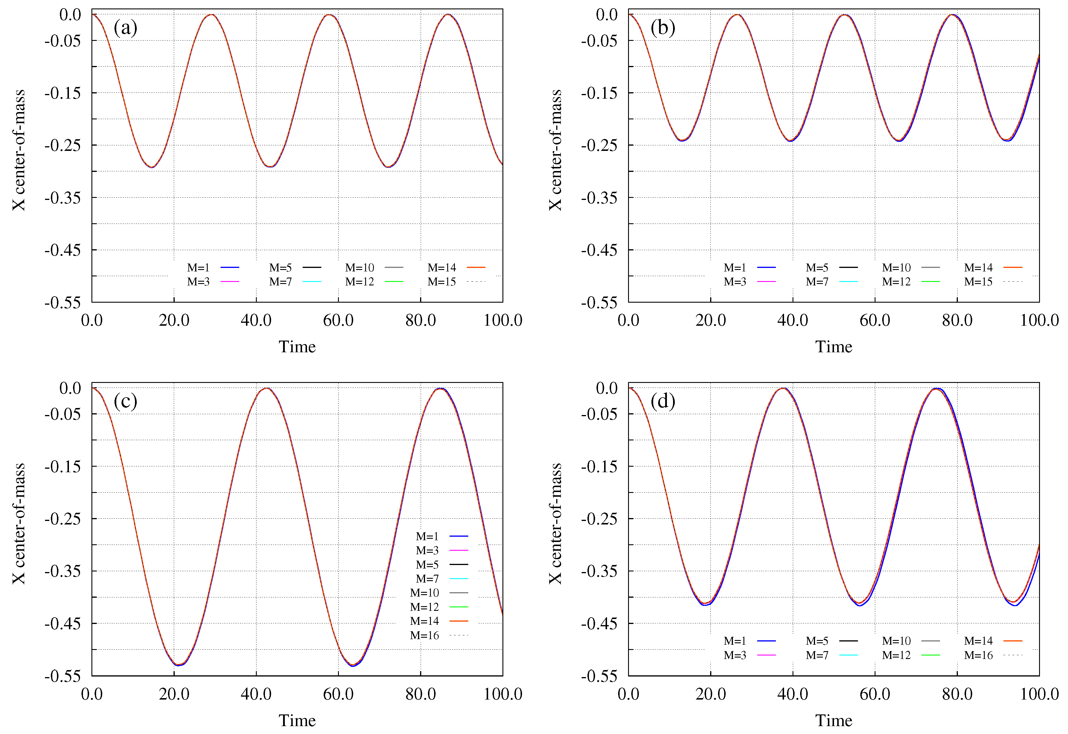
We begin with the dynamics of bosons in the annulus. Following the sudden tilt of the potential, the bosons start to flow to the left. To quantify their sloshing dynamics, Figure 1 shows the time-dependent center-of-mass, , for the two barrier heights, and , and the two interaction strengths, and [we mention that due to the reflection symmetry]. The dynamics of appears to be almost periodic and rather simple. We examine the amplitude and frequency of oscillations. It is useful to compare the amplitude of the center-of-mass motion with the radius of the (un-tilted) annulus. The radius of the density at its maximal value, R, is determined numerically using a computation with a resolution of grid points as for , and for [19]. From Figure 1 we see that the amplitude is about 13– of the radius, implying a mild sloshing of the density along the tilted annulus. The amplitude increases with the radius of the annulus and decreases with the interaction strength, where the latter implies that it is more difficult to compress the BEC for a stronger interaction. The decrease of the frequency of oscillations with R () and increase with are compatible with angular excitations, also see [19]. Last but not least, convergence with M is clearly seen. In fact, here already orbitals accurately describe the center-of-mass dynamics for short and intermediate times, and orbitals for all times.
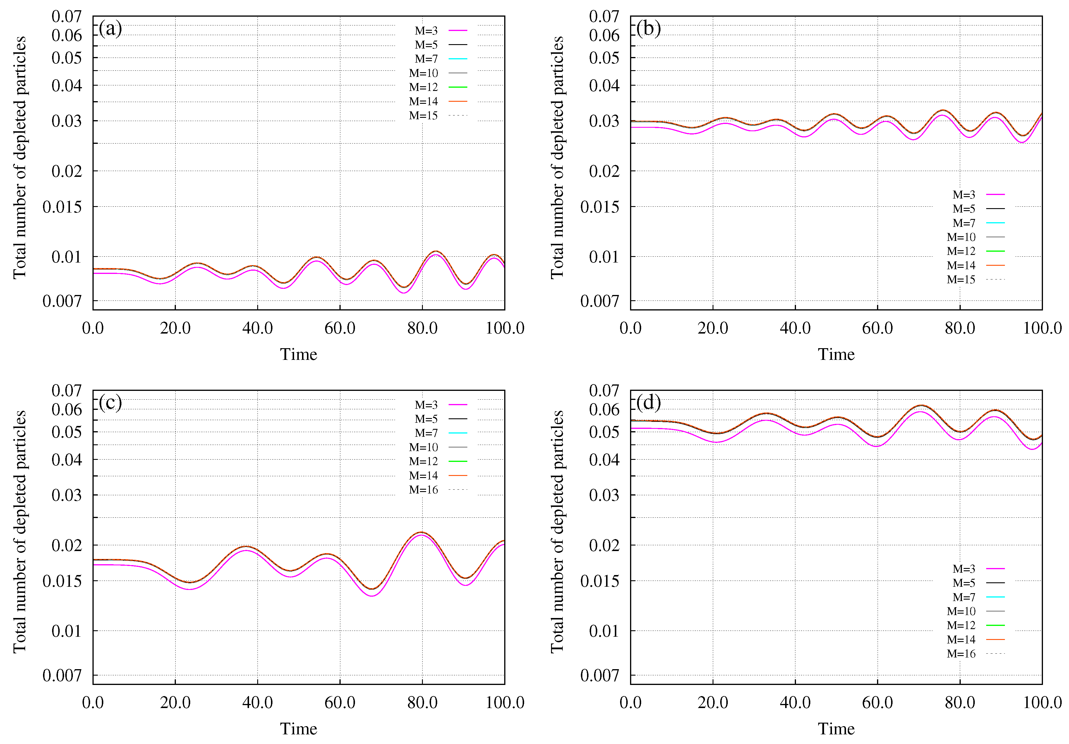
Figure 2 depicts the total number of depleted particles, , out of bosons in the tilted annulus. During the dynamics, the depletion is rather small, ranging from less than of a particle out of particles () for to less than of a particle out of particles () for . Generally, the depletion increases with the annulus radius and interacting strength, implying angular excitations, see [19]. Finally, convergence with M is clearly seen. Now, orbitals nicely follow and orbitals accurately describe the depletion dynamics, see Figure 2. The small amount of time-dependent depletion is in line with the accurate description of the center-of-mass dynamics by time adaptive orbitals, see Figure 1. Let us continue to the variances.
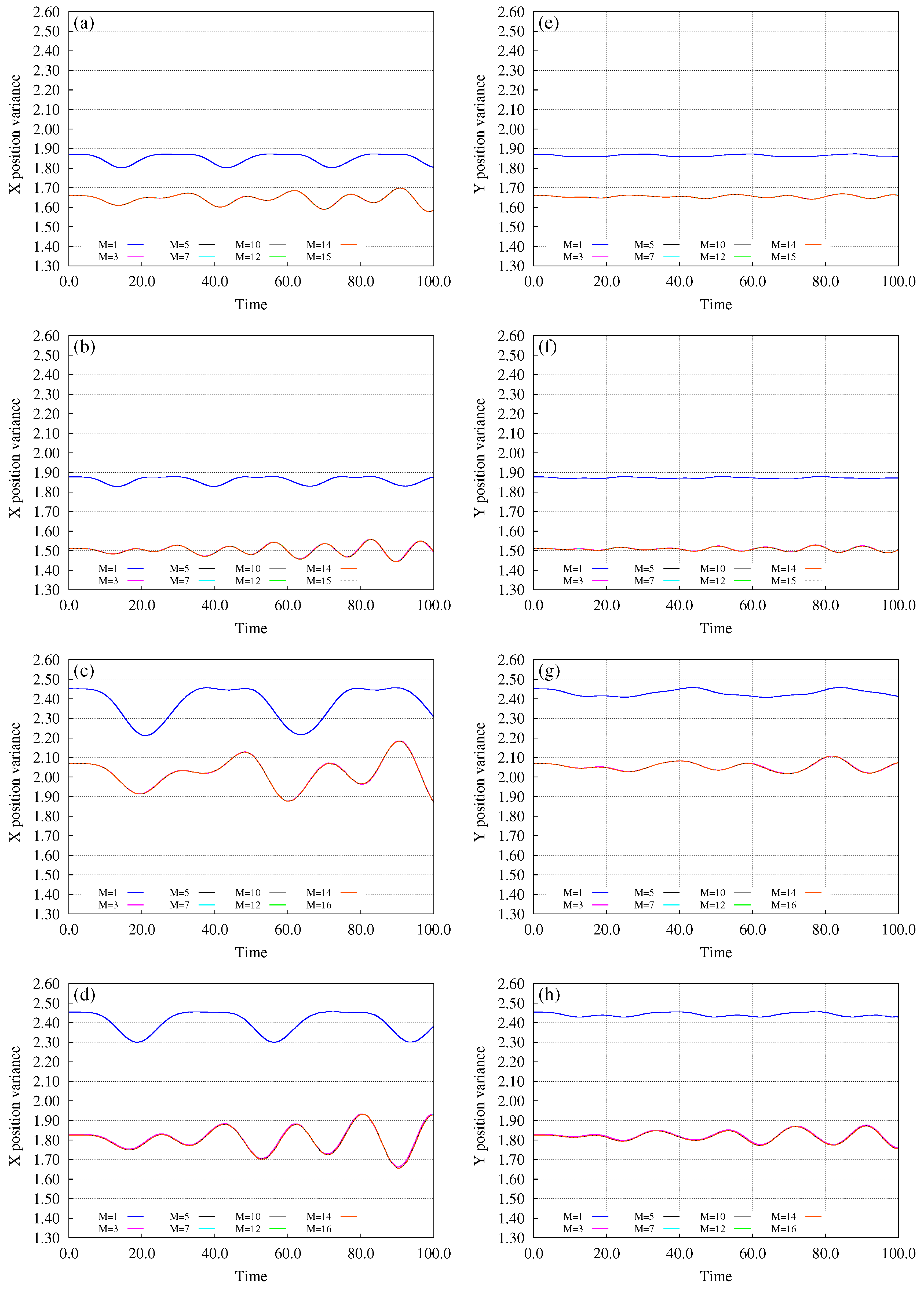
Figure 3 plots the time-dependent many-particle position variance per particle, and , for the two barrier heights and two interaction strengths. There are several features that immediately are seen. First, since rotational symmetry is lifted, the dynamics of respective quantities along the x-axis and y-axis are different [note that at the variances because the initial condition is the ground state of the un-tilted, isotropic annulus]. The mean-field () and many-body () values are clearly separated from each other, and the former lie about 10– above the latter depending on the repulsion strength and barrier height, also see [11,19]. This is despite the small amount of depletion, see Figure 2. Furthermore, the many-body and mean-field variances do not cross each other, see Figure 3, indicating that the dynamics is mild and sufficiently close to the ground state and low-lying manifold of excited states (compare to [18] with interaction-quench dynamics in a single trap).
The mean-field position variance accounts for the geometry of the annulus and shape of the density and weakly depends on the interaction strength. The many-body position variance incorporates the (small amount of) depletion and hence strongly depends on the interaction strength. Both the mean-field and many-body variances oscillate with a relatively small amplitude, albeit with a different frequencies’ content, see in this respect [20]. This amplitude slightly decreases with the repulsion strength, which correlates with the dependence of the center-of-mass dynamics on the interaction strength, see Figure 1. Moreover, the amplitude of oscillations of the y-axis variances is smaller than that of the x-axis variances, since the sloshing dynamics is primarily along the x direction. Last but not least is the so-called opposite anisotropy of the (position) variance [18]. During the dynamics, there can occur instances where at the many-body level () whereas at the mean-field level () [or, in principle, vice versa, i.e., at the many-body level whereas at the mean-field level]. Examples for the former can be readily found for , , see Figure 3c,g around , and for , , see Figure 3d,h around , signifying among others that correlations ‘win’ over shape. Finally, we see that already orbitals accurately describe the dynamics of the position variance.
We move to the momentum variance and also make contact with the results of the position variance. Figure 4 displays the many-particle momentum variance per particle, and , for , and , . Just like the results of the position variance, since rotational symmetry is lifted the dynamics of respective quantities along the x-axis and y-axis are different [the initial conditions imply at ]. The mean-field () and many-body () values are, again, separated from each other, but now the former lie below the later, and there is only about 1– of a difference depending on the repulsion strength and barrier height, also see [12,19]. Thus, the momentum variance rather weakly depends on the (small amount of) depletion. This is because the matrix elements in (20) are typically smaller with the momentum operator than with the position operator. Yet, despite their small difference, the many-body and mean-field momentum variances do not cross each other, see Figure 4 (contrast with the interaction-quench dynamics in a single trap in [18]).
It is instructive to analyze the momentum-variance dynamics at short times. Whereas primarily increases, mainly decreases. This matches the geometry of the sloshing dynamics in the tilted annulus, in which bosons from the ‘north’ and ‘south’ poles (on the y-axis) start to move to the left and accumulate in the ‘west’ pole (on the x-axis), and that the cross section of the rim of an annulus is enlarged when moving away from the center of the annulus. In other words, the dynamics of the momentum variances at short times when moving to the left reflects the relative localization of the bosons in the x direction and the effective broadening of the wavepacket along the y direction. Both the mean-field and many-body variances oscillate with a very small amplitude, note the scale on the y-axis in Figure 4. The high-frequency oscillations mark high-energy radial excitations across the (tight) annulus rim [19]. Like for the position variance, the amplitude of oscillations of the y-axis momentum variances is smaller than that of the x-axis momentum variances. Finally, we see that already orbitals accurately describe the dynamics of the momentum variance; the difference to the results is lower than .
We now move to the angular-momentum variance and an interesting inter-connection with the momentum variance. Figure 5 presents the many-particle angular-momentum variance per particle, , for the two barrier heights, and , and the two interaction strengths, and . There are several features seen in the dynamics. Since rotational symmetry is lifted, expect for the initial conditions at (the values of the minima for , see below, are close to but not 0). The dynamics of appears to be almost periodic and rather regular, more than that for the respective position and momentum variances, compare to Figure 3 and Figure 4. On the other end, focusing on the dynamics of the center-of-mass in Figure 1, one can clearly observe correlation between the two quantities; Whenever has a minimum, i.e., the bosons are maximally localized to the left, has a maximum, and whenever has a maximum (which value is about 0), i.e., the bosons are momentarily, approximately equally distributed along the annulus, has a minimum (which value, as mentioned above, is close to 0). Furthermore, the frequencies of the two quantities as well as their relative amplitudes as a function of the barrier height and interaction strength are alike. These observations call for a dedicated analysis.
To shed light on the above dynamics of the angular-momentum variance, see Figure 5, we analyze the translational properties of variances in Appendix A. Whereas the position variances and, trivially, the momentum variances, are translationally invariant, this invariance does not hold for the angular-momentum variance. If a wavepacket prepared in the origin has angular-momentum variance , then several terms are added when the wavepacket is translated to the point in plane, and angular-momentum variance is thereafter computed, see Equation (A3). Now, if this wavepacket is rotationally symmetric, i.e., , then several of the terms in (A3) vanish due to spatial symmetry and we are left with the appealing relation, [Equation (A4)], connecting the angular-momentum variance of localized at and of at the origin. The meaning of this relation is that the momentum variances, and , together with the spatial translations along the y-axis and x-axis, respectively, determine the angular-momentum variance of a translated wavepacket (rotationally symmetric at the origin).
Returning to and combining Figure 5 for the angular-momentum variance, Figure 1 for the center-of-mass dynamics, and Figure 4e–h for , we can now discuss and explain their inter-connection. Explicitly, the center-of-mass dynamics is analogous to translating the wavepacket along the x-axis (back and forth to the left), hence, according to Equation (A4), is needed. This is why the dependencies of the frequency and amplitude of oscillations of on the barrier height and interaction strength nicely follow, respectively, those of , compare Figure 1 and Figure 5. What is the role of then? The momentum variance helps us understand the deviations between the many-body and mean-field results in Figure 5. We see that the maxima of the many-body () are larger than the maxima of the mean-field (). The difference is about 7– (compare to the low depletion, Figure 2), depending on and , and follows the respective trend of the many-body and mean-field results for , see Figure 4e–h. We note that, although the wavepacket describing the bosons dynamics in the tilted annulus is not a translated, rotationally invariant wavepacket, and the values of deviations (in percents) between the many-body and mean-field results are actually larger for (at the maxima) than for , we find the above analytically based analysis to well explain the numerical findings and trends. Last but not least, a close inspection of the many-body and mean-field curves of the angular-momentum variance in Figure 5 shows that there are instances when they cross each other, i.e., one is smaller or larger than the other. This is in contrast with the non-crossing of the many-body and mean-field position and momentum variances, see Figure 3 and Figure 4, respectively. Finally, we find that already time-adaptive orbitals accurately describe the dynamics of the angular-momentum variance.
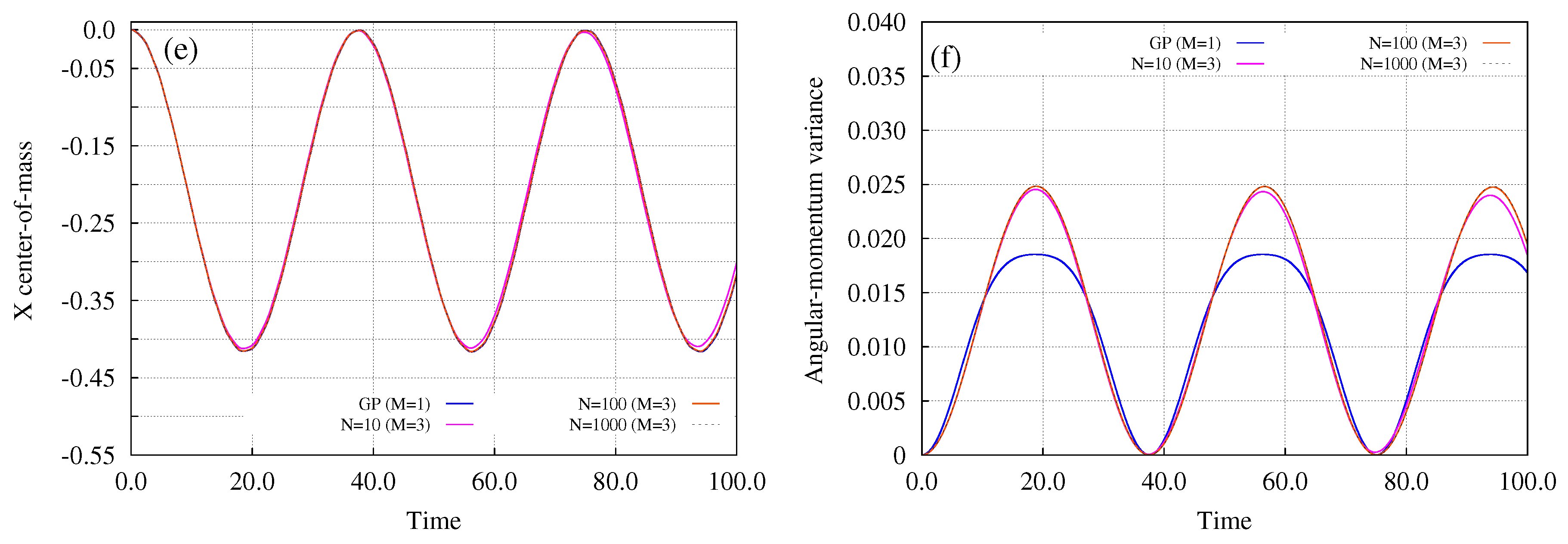
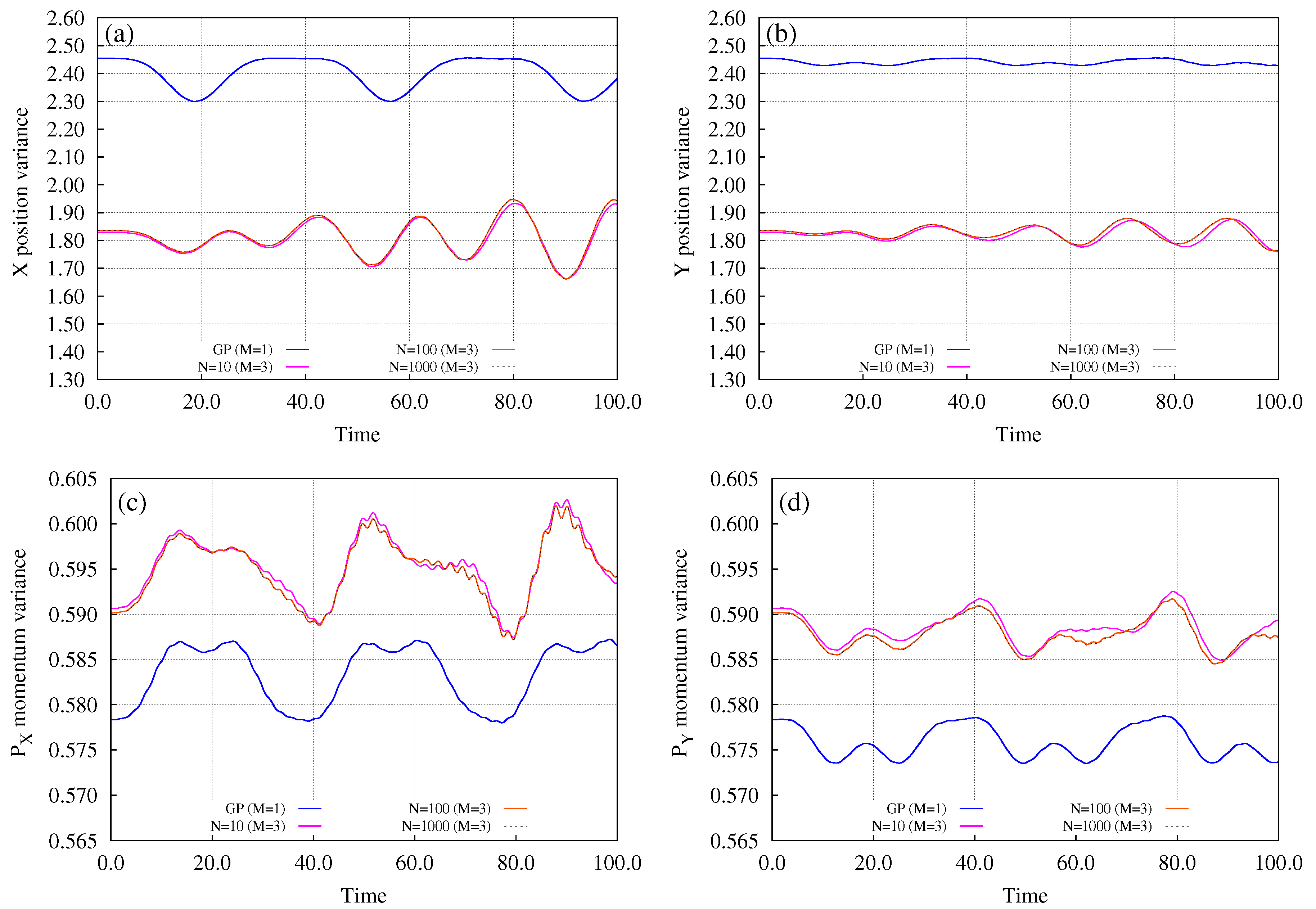
Our investigations are nearing their end, what is left to explore is the behavior of the position, momentum, and angular-momentum variances at the particle limit. Which of the above-described detailed findings, plotted in Figure 1, Figure 2, Figure 3, Figure 4 and Figure 5 for a rather small ( bosons) yet weakly depleted BEC, survive this limit? To answer the question, we concentrate on the system with the higher barrier, , and stronger interaction (for bosons), . We hence fix the interaction parameter , and compute and compare the dynamics for , , and bosons using time-adaptive orbitals. We have seen for bosons that time-adaptive orbitals accurately describe the variances. This implies that, keeping the interaction parameter fixed while increasing the number of particles N, using time-adaptive orbitals for calculating the variances will be (at least) as accurate as for particles, see in this respect [24]. Before we proceed, a methodological remark. Examining the convergence of properties with the number of particles for , , and bosons is (still) far away from infinity, see in this respect [15]. We hence use, interchangeably, the term en route to the particle limit. We shall see below that, in effect, the particle limit is practically well achieved for the variances already for bosons.
Figure 6 prints the total number of depleted particles, , for , , and bosons for and using time-adaptive orbitals. Convergence of the number of depleted particles with N is nicely seen. Since converges to a finite (and small) value with N, the bosons are becoming condensed in the limit of an infinite number of particles, i.e., as , at least up to the maximal time of the computation, .
Figure 7 exhibits the position variances per particle, and , momentum variances per particle, and , angular-momentum variance per particle, , and the expectation value of the center-of-mass, , for , , and bosons and for and using time-adaptive orbitals. Once again, convergence of each of the quantities with N is clearly seen. Yet, whereas the center-of-mass dynamics converges to the mean-field dynamics when the number of particles is increased, the variances exhibit many-body dynamics which converges nicely with N, but not to the respective mean-field dynamics. Beyond that, all the above results, for the frequencies, amplitudes, anisotropies, inter-connections, and particularly the differences between the many-body and mean-field position, momentum, and angular-momentum variances persist at the limit of infinite number of particles, despite the bosons becoming condensed. This brings the present analysis to an end.
4. Summary and Outlook
In the present work we studied, analytically and numerically, the position, momentum, and especially the angular-momentum variance of interacting bosons trapped in a two-dimensional anisotropic trap for static and dynamic scenarios. Explicitly, we investigated the ground state of the anisotropic harmonic-interaction model in two spatial dimensions analytically and researched the out-of-equilibrium dynamics of repulsive bosons in tilted two-dimensional annuli numerically accurately by using the MCTDHB method.
The differences between the variances at the mean-field level, which are attributed to the shape of the density per particle, and the respective variances at the many-body level, which incorporate a small amount of depletion outside the condensed mode, were used to characterize sometimes large position, momentum, and angular-momentum correlations in the BEC for finite systems and at the limit of an infinite number of particles where the bosons are condensed. Finally, we also explored and utilized inter-connections between the variances, particularly between the angular-momentum and momentum variances, through the analysis of their translational properties.
There are many intriguing directions to follow out of which we list three below. First, variances of BECs in the rotating frame of reference in which high-lying excitations become low-energy excitations and even the ground state. Second, angular-momentum variance of a BEC flowing past an obstacle in which the mean angular-momentum variance vanishes. And third, variances in three-dimensional geometries lacking lower-dimensional analogs, such as a Möbius strip. In all these cases, whether considering a few interacting bosons or a BEC in the particle limit, interesting and exciting results are expected.
Funding
This research was funded by Israel Science Foundation (Grant No. 600/15).
Acknowledgments
This research was supported by the Israel Science Foundation (Grant No. 600/15). We thank Kaspar Sakmann, Anal Bhowmik, Sudip Haldar, and Raphael Beinke for discussions. Computation time on the BwForCluster, the High Performance Computing system Hive of the Faculty of Natural Sciences at University of Haifa, and the Cray XC40 system Hazelhen at the High Performance Computing Center Stuttgart (HLRS) is gratefully acknowledged.
Conflicts of Interest
The authors declare no conflict of interest.
Appendix A. Variances and Translations
Consider the many-particle translation operator in two spatial dimensions , where and . Its operation on a multi-particle wavefunction is given by . What are the implications on the variances when computed with respect to the translated wavefunction ?
For the position operator (and equivalently for ) we have and , implying that
Trivially for the momentum operator (and equivalently for ) one has
i.e., both the position variance and momentum variance are translationally invariant.
For the angular-momentum operator the situation is more interesting. From and we have
Equation (A3) deserves a discussion. In turn, even for the ground state of an interacting many-boson system in a rotationally symmetric [for which holds] but otherwise translated trap, the angular-momentum variance
differs at the many-body level and mean-field level of theory, i.e., when and . This is, as can be seen in (A4), because of the respective many-body and mean-field momentum variances, and . The analytical result (A4) is employed to analyze the numerical findings for the time-dependent angular-momentum variance in the main text. Generally in the absence of spatial symmetries, see Equation (A3), more terms contribute to the translated angular-momentum variance.
References
- Cornell, E.A.; Wieman, C.E. Nobel Lecture: Bose–Einstein condensation in a dilute gas, the first 70 years and some recent experiments. Rev. Mod. Phys. 2002, 74, 875. [Google Scholar] [CrossRef]
- Ketterle, W. Nobel lecture: When atoms behave as waves: Bose–Einstein condensation and the atom laser. Rev. Mod. Phys. 2002, 74, 1131. [Google Scholar] [CrossRef]
- Dalfovo, F.; Giorgini, S.; Pitaevskii, L.P.; Stringari, S. Theory of Bose–Einstein condensation in trapped gases. Rev. Mod. Phys. 1999, 71, 463. [Google Scholar] [CrossRef]
- Leggett, A.J. Bose–Einstein condensation in the alkali gases: Some fundamental concepts. Rev. Mod. Phys. 2001, 73, 307. [Google Scholar] [CrossRef]
- Bloch, I.; Dalibard, J.; Zwerger, W. Many-body physics with ultracold gases. Rev. Mod. Phys. 2008, 80, 885. [Google Scholar] [CrossRef]
- Castin, Y.; Dum, R. Low-temperature Bose–Einstein condensates in time-dependent traps: Beyond the U(1) symmetry breaking approach. Phys. Rev. A 1998, 57, 3008. [Google Scholar] [CrossRef]
- Lieb, E.H.; Seiringer, R.; Yngvason, J. Bosons in a trap: A rigorous derivation of the Gross-Pitaevskii energy functional. Phys. Rev. A 2000, 61, 043602. [Google Scholar] [CrossRef] [Green Version]
- Lieb, E.H.; Seiringer, R. Proof of Bose–Einstein Condensation for Dilute Trapped Gases. Phys. Rev. Lett. 2002, 88, 170409. [Google Scholar] [CrossRef]
- Erdos, L.; Schlein, B.; Yau, H.-T. Rigorous Derivation of the Gross-Pitaevskii Equation. Phys. Rev. Lett. 2007, 98, 040404. [Google Scholar] [CrossRef]
- Erdos, L.; Schlein, B.; Yau, H.-T. Derivation of the cubic non-linear Schrödinger equation from quantum dynamics of many-body systems. Invent. Math. 2007, 167, 515. [Google Scholar] [CrossRef]
- Klaiman, S.; Alon, O.E. Variance as a sensitive probe of correlations. Phys. Rev. A 2015, 91, 063613. [Google Scholar] [CrossRef]
- Klaiman, S.; Streltsov, A.I.; Alon, O.E. Uncertainty product of an out-of-equilibrium many-particle system. Phys. Rev. A 2016, 93, 023605. [Google Scholar] [CrossRef] [Green Version]
- Klaiman, S.; Cederbaum, L.S. Overlap of exact and Gross-Pitaevskii wave functions in Bose–Einstein condensates of dilute gases. Phys. Rev. A 2016, 94, 063648. [Google Scholar] [CrossRef]
- Michelangeli, A.; Olgiati, A. Mean-field quantum dynamics for a mixture of Bose–Einstein condensates. Anal. Math. Phys. 2017, 7, 377. [Google Scholar] [CrossRef]
- Cederbaum, L.S. Exact many-body wave function and properties of trapped bosons in the particle limit. Phys. Rev. A 2017, 96, 013615. [Google Scholar] [CrossRef]
- Alon, O.E. Solvable model of a generic trapped mixture of interacting bosons: reduced density matrices and proof of Bose–Einstein condensation. J. Phys. A 2017, 50, 295002. [Google Scholar] [CrossRef]
- Coleman, A.J.; Yukalov, V.I. Reduced Density Matrices: Coulson’s Challenge; Lectures Notes in Chemistry; Springer: Berlin, Germany, 2000; Volume 72. [Google Scholar]
- Klaiman, S.; Beinke, R.; Cederbaum, L.S.; Streltsov, A.I.; Alon, O.E. Variance of an anisotropic Bose–Einstein condensate. Chem. Phys. 2018, 509, 45. [Google Scholar] [CrossRef]
- Alon, O.E. Condensates in annuli: Dimensionality of the variance. Mol. Phys. 2019, 117, 2108. [Google Scholar] [CrossRef]
- Theisen, M.; Streltsov, A.I. Many-body excitations and deexcitations in trapped ultracold bosonic clouds. Phys. Rev. A 2016, 94, 053622. [Google Scholar] [CrossRef] [Green Version]
- Haldar, S.K.; Alon, O.E. Impact of the range of the interaction on the quantum dynamics of a bosonic Josephson junction. Chem. Phys. 2018, 509, 72. [Google Scholar] [CrossRef]
- Haldar, S.K.; Alon, O.E. Many-body quantum dynamics of an asymmetric bosonic Josephson junction. New J. Phys. 2019, 21, 103037. [Google Scholar] [CrossRef] [Green Version]
- Cosme, J.G.; Weiss, C.; Brand, J. Center-of-mass motion as a sensitive convergence test for variational multimode quantum dynamics. Phys. Rev. A 2016, 94, 043603. [Google Scholar] [CrossRef] [Green Version]
- Alon, O.E.; Cederbaum, L.S. Attractive Bose–Einstein condensates in anharmonic traps: Accurate numerical treatment and the intriguing physics of the variance. Chem. Phys. 2018, 515, 287. [Google Scholar] [CrossRef]
- Sakmann, K.; Schmiedmayer, J. Conserving symmetries in Bose–Einstein condensate dynamics requires many-body theory. arXiv 2018, arXiv:1802.03746v2. [Google Scholar]
- Klaiman, S.; Streltsov, A.I.; Alon, O.E. Solvable Model of a Generic Trapped Mixture of Interacting Bosons: Many-Body and Mean-Field Properties. J. Phys. Conf. Ser. 2018, 999, 012013. [Google Scholar] [CrossRef]
- Hall, R.L. Some exact solutions to the translation-invariant N-body problem. J. Phys. A 1978, 11, 1227. [Google Scholar] [CrossRef]
- Hall, R.L. Exact solutions of Schrödinger’s equation for translation-invariant harmonic matter. J. Phys. A 1978, 11, 1235. [Google Scholar] [CrossRef]
- Cohen, L.; Lee, C. Exact reduced density matrices for a model problem. J. Math. Phys. 1985, 26, 3105. [Google Scholar] [CrossRef]
- Osadchii, M.S.; Muraktanov, V.V. The System of Harmonically Interacting Particles: An Exact Solution of the Quantum-Mechanical Problem. Int. J. Quant. Chem. 1991, 39, 173. [Google Scholar] [CrossRef]
- Załuska-Kotur, M.A.; Gajda, M.; Orłowski, A.; Mostowski, J. Soluble model of many interacting quantum particles in a trap. Phys. Rev. A 2000, 61, 033613. [Google Scholar] [CrossRef] [Green Version]
- Yan, J. Harmonic Interaction Model and Its Applications in Bose–Einstein Condensation. J. Stat. Phys. 2003, 113, 623. [Google Scholar] [CrossRef]
- Gajda, M. Criterion for Bose–Einstein condensation in a harmonic trap in the case with attractive interactions. Phys. Rev. A 2006, 73, 023603. [Google Scholar] [CrossRef]
- Armstrong, J.R.; Zinner, N.T.; Fedorov, D.V.; Jensen, A.S. Analytic harmonic approach to the N-body problem. J. Phys. B 2011, 44, 055303. [Google Scholar] [CrossRef]
- Armstrong, J.R.; Zinner, N.T.; Fedorov, D.V.; Jensen, A.S. Virial expansion coefficients in the harmonic approximation. Phys. Rev. E 2012, 86, 021115. [Google Scholar] [CrossRef] [Green Version]
- Schilling, C. Natural orbitals and occupation numbers for harmonium: Fermions versus bosons. Phys. Rev. A 2013, 88, 042105. [Google Scholar] [CrossRef]
- Benavides-Riveros, C.L.; Toranzo, I.V.; Dehesa, J.S. Entanglement in N-harmonium: Bosons and fermions. J. Phys. B 2014, 47, 195503. [Google Scholar] [CrossRef]
- Bouvrie, P.A.; Majtey, A.P.; Tichy, M.C.; Dehesa, J.S.; Plastino, A.R. Entanglement and the Born-Oppenheimer approximation in an exactly solvable quantum many-body system. Eur. Phys. J. D 2014, 68, 346. [Google Scholar] [CrossRef]
- Armstrong, J.R.; Volosniev, A.G.; Fedorov, D.V.; Jensen, A.S.; Zinner, N.T. Analytic solutions of topologically disjoint systems. J. Phys. A 2015, 48, 085301. [Google Scholar] [CrossRef]
- Schilling, C.; Schilling, R. Number-parity effect for confined fermions in one dimension. Phys. Rev. 2016, 93, 021601. [Google Scholar] [CrossRef] [Green Version]
- Klaiman, S.; Streltsov, A.I.; Alon, O.E. Solvable model of a trapped mixture of Bose–Einstein condensates. Chem. Phys. 2017, 482, 362. [Google Scholar] [CrossRef]
- Sakmann, K.; Streltsov, A.I.; Alon, O.E.; Cederbaum, L.S. Exact ground state of finite Bose–Einstein condensates on a ring. Phys. Rev. A 2005, 72, 033613. [Google Scholar] [CrossRef]
- Gupta, S.; Murch, K.W.; Moore, K.L.; Purdy, T.P.; Stamper-Kurn, D.M. Bose–Einstein Condensation in a Circular Waveguide. Phys. Rev. Lett. 2005, 95, 143201. [Google Scholar] [CrossRef] [PubMed]
- Cozzini, M.; Jackson, B.; Stringari, S. Vortex signatures in annular Bose–Einstein condensates. Phys. Rev. A 2006, 73, 013603. [Google Scholar] [CrossRef]
- Bao, C.G. Oscillation bands of Bose–Einstein condensates on a ring: Beyond the mean-field theory. Phys. Rev. A 2007, 75, 063626. [Google Scholar] [CrossRef]
- Smyrnakis, J.; Bargi, S.; Kavoulakis, G.M.; Magiropoulos, M.; Kärkkäinen, K.; Reimann, S.M. Mixtures of Bose Gases Confined in a Ring Potential. Phys. Rev. Lett. 2009, 103, 100404. [Google Scholar] [CrossRef] [PubMed] [Green Version]
- Halkyard, P.L.; Jones, M.P.A.; Gardiner, S.A. Rotational response of two-component Bose–Einstein condensates in ring traps. Phys. Rev. A 2010, 81, 061602. [Google Scholar] [CrossRef]
- Mathey, L.; Ramanathan, A.; Wright, K.C.; Muniz, S.R.; Phillips, W.D.; Clark, C.W. Phase fluctuations in anisotropic Bose–Einstein condensates: From cigars to rings. Phys. Rev. A 2010, 82, 033607. [Google Scholar] [CrossRef]
- Sherlock, B.E.; Gildemeister, M.; Owen, E.; Nugent, E.; Foot, C.J. Time-averaged adiabatic ring potential for ultracold atoms. Phys. Rev. A 2011, 83, 043408. [Google Scholar] [CrossRef] [Green Version]
- Zöllner, S.; Bruun, G.M.; Pethick, C.J.; Reimann, S.M. Bosonic and Fermionic Dipoles on a Ring. Phys. Rev. Lett. 2011, 107, 035301. [Google Scholar] [CrossRef]
- Adhikari, S.K. Dipolar Bose–Einstein condensate in a ring or in a shell. Phys. Rev. A 2012, 85, 053631. [Google Scholar] [CrossRef]
- Dubessy, R.; Liennard, T.; Pedri, P.; Perrin, H. Critical rotation of an annular superfluid Bose–Einstein condensate. Phys. Rev. A 2012, 86, 011602. [Google Scholar] [CrossRef]
- Woo, S.J.; Son, Y.-W. Vortex dynamics in an annular Bose–Einstein condensate. Phys. Rev. A 2012, 86, 011604. [Google Scholar] [CrossRef]
- Moulder, S.; Beattie, S.; Smith, R.P.; Tammuz, N.; Hadzibabic, Z. Quantized supercurrent decay in an annular Bose–Einstein condensate. Phys. Rev. A 2012, 86, 013629. [Google Scholar] [CrossRef]
- Toikka, L.A.; Suominen, K.-A. Snake instability of ring dark solitons in toroidally trapped Bose–Einstein condensates. Phys. Rev. A 2013, 87, 043601. [Google Scholar] [CrossRef]
- Eckel, S.; Lee, J.G.; Jendrzejewski, F.; Murray, N.; Clark, C.W.; Lobb, C.J.; Phillips, W.D.; Edwards, M.; Campbell, G.K. Hysteresis in a quantized superfluid ‘atomtronic’ circuit. Nature 2014, 506, 200. [Google Scholar] [CrossRef]
- Mateo, A.M.; Gallemí, A.; Guilleumas, M.; Mayol, R. Persistent currents supported by solitary waves in toroidal Bose–Einstein condensates. Phys. Rev. A 2015, 91, 063625. [Google Scholar] [CrossRef]
- Kolář, M.; Opatrný, T.; Das, K.K. Criticality and spin squeezing in the rotational dynamics of a Bose–Einstein condensate on a ring lattice. Phys. Rev. A 2015, 92, 043630. [Google Scholar] [CrossRef]
- Roy, A.; Angom, D. Geometry-induced modification of fluctuation spectrum in quasi-two-dimensional condensates. New J. Phys. 2016, 18, 083007. [Google Scholar] [CrossRef] [Green Version]
- Roussou, A.; Smyrnakis, J.; Magiropoulos, M.; Efremidis, N.K.; Kavoulakis, G.M. Rotating Bose–Einstein condensates with a finite number of atoms confined in a ring potential: Spontaneous symmetry breaking beyond the mean-field approximation. Phys. Rev. A 2017, 95, 033606. [Google Scholar] [CrossRef]
- Wang, J.-G.; Xu, L.-L.; Yang, S.-J. Ground-state phases of the spin-orbit-coupled spin-1 Bose gas in a toroidal trap. Phys. Rev. A 2017, 96, 033629. [Google Scholar] [CrossRef] [Green Version]
- Guenther, N.-E.; Massignan, P.; Fetter, A.L. Quantized superfluid vortex dynamics on cylindrical surfaces and planar annuli. Phys. Rev. A 2017, 96, 063608. [Google Scholar] [CrossRef] [Green Version]
- Roy, A.; Angom, D. Ramifications of topology and thermal fluctuations in quasi-2D condensates. J. Phys. B 2017, 50, 225301. [Google Scholar] [CrossRef] [Green Version]
- Padavić, K.; Sun, K.; Lannert, C.; Vishveshwara, S. Physics of hollow Bose–Einstein condensates. Europhys. Lett. 2017, 120, 20004. [Google Scholar] [CrossRef]
- Eckel, S.; Kumar, A.; Jacobson, T.; Spielman, I.B.; Campbell, G.K. A Rapidly Expanding Bose–Einstein Condensate: An Expanding Universe in the Lab. Phys. Rev. X 2018, 8, 021021. [Google Scholar] [CrossRef] [PubMed]
- Sun, K.; Padavić, K.; Yang, F.; Vishveshwara, S.; Lannert, C. Static and dynamic properties of shell-shaped condensates. Phys. Rev. A 2018, 98, 013609. [Google Scholar] [CrossRef] [Green Version]
- Streltsov, A.I.; Alon, O.E.; Cederbaum, L.S. Role of Excited States in the Splitting of a Trapped Interacting Bose–Einstein Condensate by a Time-Dependent Barrier. Phys. Rev. Lett. 2007, 99, 030402. [Google Scholar] [CrossRef] [PubMed]
- Alon, O.E.; Streltsov, A.I.; Cederbaum, L.S. Multiconfigurational time-dependent Hartree method for bosons: Many-body dynamics of bosonic systems. Phys. Rev. A 2008, 77, 033613. [Google Scholar] [CrossRef] [Green Version]
- Lode, A.U.J.; Lévêque, C.; Madsen, L.B.; Streltsov, A.I.; Alon, O.E. Multiconfigurational time-dependent Hartree approaches for indistinguishable particles. arXiv 2019, arXiv:1908.03578v1. [Google Scholar]
- Alon, O.E.; Streltsov, A.I.; Cederbaum, L.S. Multiconfigurational time-dependent Hartree method for mixtures consisting of two types of identical particles. Phys. Rev. A. 2007, 76, 062501. [Google Scholar] [CrossRef]
- Sakmann, K.; Streltsov, A.I.; Alon, O.E.; Cederbaum, L.S. Exact Quantum Dynamics of a Bosonic Josephson Junction. Phys. Rev. Lett. 2009, 103, 220601. [Google Scholar] [CrossRef] [Green Version]
- Grond, J.; Schmiedmayer, J.; Hohenester, U. Optimizing number squeezing when splitting a mesoscopic condensate. Phys. Rev. A 2009, 79, 021603. [Google Scholar] [CrossRef] [Green Version]
- Lode, A.U.J.; Sakmann, K.; Alon, O.E.; Cederbaum, L.S.; Streltsov, A.I. Numerically exact quantum dynamics of bosons with time-dependent interactions of harmonic type. Phys. Rev. A 2012, 86, 063606. [Google Scholar] [CrossRef] [Green Version]
- Krönke, S.; Cao, L.; Vendrell, O.; Schmelcher, P. Non-equilibrium quantum dynamics of ultra-cold atomic mixtures: the multi-layer multi-configuration time-dependent Hartree method for bosons. New J. Phys. 2013, 15, 063018. [Google Scholar] [CrossRef]
- Cao, L.; Krönke, S.; Vendrell, O.; Schmelcher, P. The multi-layer multi-configuration time-dependent Hartree method for bosons: Theory, implementation, and applications. J. Chem. Phys. 2013, 139, 134103. [Google Scholar] [CrossRef] [Green Version]
- Streltsov, A.I. Quantum systems of ultracold bosons with customized interparticle interactions. Phys. Rev. A 2012, 88, 041602. [Google Scholar] [CrossRef]
- Streltsova, O.I.; Alon, O.E.; Cederbaum, L.S.; Streltsov, A.I. Generic regimes of quantum many-body dynamics of trapped bosonic systems with strong repulsive interactions. Phys. Rev. A 2014, 89, 061602. [Google Scholar] [CrossRef] [Green Version]
- Fischer, U.R.; Lode, A.U.J.; Chatterjee, B. Condensate fragmentation as a sensitive measure of the quantum many-body behavior of bosons with long-range interactions. Phys. Rev. A 2015, 91, 063621. [Google Scholar] [CrossRef]
- Fasshauer, E.; Lode, A.U.J. Multiconfigurational time-dependent Hartree method for fermions: Implementation, exactness, and few-fermion tunneling to open space. Phys. Rev. A 2016, 93, 033635. [Google Scholar] [CrossRef] [Green Version]
- Lode, A.U.J. Multiconfigurational time-dependent Hartree method for bosons with internal degrees of freedom: Theory and composite fragmentation of multicomponent Bose–Einstein condensates. Phys. Rev. A 2016, 93, 063601. [Google Scholar] [CrossRef]
- Sakmann, K.; Kasevich, M. Single-shot simulations of dynamic quantum many-body systems. Nat. Phys. 2016, 12, 451. [Google Scholar] [CrossRef]
- Cao, L.; Bolsinger, V.; Mistakidis, S.I.; Koutentakis, G.M.; Krönke, S.; Schurer, J.M.; Schmelcher, P. A unified ab initio approach to the correlated quantum dynamics of ultracold fermionic and bosonic mixtures. J. Chem. Phys. 2017, 147, 044106. [Google Scholar] [CrossRef] [PubMed]
- Bolsinger, V.J.; Krönke, S.; Schmelcher, P. Beyond mean-field dynamics of ultra-cold bosonic atoms in higher dimensions: facing the challenges with a multi-configurational approach. J. Phys. B 2017, 50, 034003. [Google Scholar] [CrossRef]
- Lévêque, C.; Madsen, L.B. Time-dependent restricted-active-space self-consistent-field theory for bosonic many-body systems. New J. Phys. 2017, 19, 043007. [Google Scholar] [CrossRef] [Green Version]
- Weiner, S.E.; Tsatsos, M.C.; Cederbaum, L.S.; Lode, A.U.J. Phantom vortices: Hidden angular momentum in ultracold dilute Bose–Einstein condensates. Sci Rep. 2017, 7, 40122. [Google Scholar] [CrossRef]
- Lode, A.U.J.; Bruder, C. Fragmented Superradiance of a Bose–Einstein Condensate in an Optical Cavity. Phys. Rev. Lett. 2017, 118, 013603. [Google Scholar] [CrossRef]
- Bolsinger, V.J.; Krönke, S.; Schmelcher, P. Ultracold bosonic scattering dynamics off a repulsive barrier: Coherence loss at the dimensional crossover. Phys. Rev. A 2017, 96, 013618. [Google Scholar] [CrossRef] [Green Version]
- Katsimiga, G.C.; Mistakidis, S.I.; Koutentakis, G.M.; Kevrekidis, P.G.; Schmelcher, P. Many-body quantum dynamics in the decay of bent dark solitons of Bose–Einstein condensates. New J. Phys. 2017, 19, 123012. [Google Scholar] [CrossRef]
- Schurer, J.M.; Negretti, A.; Schmelcher, P. Unraveling the Structure of Ultracold Mesoscopic Collinear Molecular Ions. Phys. Rev. Lett. 2017, 119, 063001. [Google Scholar] [CrossRef]
- Chen, J.; Schurer, J.M.; Schmelcher, P. Entanglement Induced Interactions in Binary Mixtures. Phys. Rev. Lett. 2018, 121, 043401. [Google Scholar] [CrossRef] [Green Version]
- Lévêque, C.; Madsen, L.B. Multispecies time-dependent restricted-active-space self-consistent-field-theory for ultracold atomic and molecular gases. J. Phys. B 2018, 51, 155302. [Google Scholar] [CrossRef]
- Roy, R.; Gammal, A.; Tsatsos, M.C.; Chatterjee, B.; Chakrabarti, B.; Lode, A.U.J. Phases, many-body entropy measures, and coherence of interacting bosons in optical lattices. Phys. Rev. A 2018, 97, 043625. [Google Scholar] [CrossRef] [Green Version]
- Elsayed, T.A.; Streltsov, A.I. Probing quantum states with momentum boosts. Phys. Rev. A 2018, 98, 013618. [Google Scholar] [CrossRef] [Green Version]
- Nguyen, J.H.V.; Tsatsos, M.C.; Luo, D.; Lode, A.U.J.; Telles, G.D.; Bagnato, V.S.; Hulet, R.G. Parametric Excitation of a Bose–Einstein Condensate: From Faraday Waves to Granulation. Phys. Rev. X 2019, 9, 011052. [Google Scholar] [CrossRef]
- Marchukov, O.V.; Fischer, U.R. Self-consistent determination of the many-body state of ultracold bosonic atoms in a one-dimensional harmonic trap. Ann. Phys. 2019, 405, 274. [Google Scholar] [CrossRef]
- Streltsov, A.I.; Streltsova, O.I. MCTDHB-Lab, Version 1.5. 2015. Available online: http://www.mctdhb-lab.com (accessed on 29 September 2019).
- Streltsov, A.I.; Cederbaum, L.S.; Alon, O.E.; Sakmann, K.; Lode, A.U.J.; Grond, J.; Streltsova, O.I.; Klaiman, S.; Beinke, R. The Multiconfigurational Time-Dependent Hartree for Bosons Package, Version 3.x. Available online: http://mctdhb.org (accessed on 29 September 2019).
- Streltsov, A.I.; Alon, O.E.; Cederbaum, L.S. General variational many-body theory with complete self-consistency for trapped bosonic systems. Phys. Rev. A 2006, 73, 063626. [Google Scholar] [CrossRef] [Green Version]
- Meyer, H.-D.; Manthe, U.; Cederbaum, L.S. The multi-configurational time-dependent Hartree approach. Chem. Phys. Lett. 1990, 165, 73. [Google Scholar] [CrossRef]
- Manthe, U.; Meyer, H.-D.; Cederbaum, L.S. Wave-packet dynamics within the multiconfiguration Hartree framework: General aspects and application to NOCl. J. Chem. Phys. 1992, 97, 3199. [Google Scholar] [CrossRef]
- Beck, M.H.; Jäckle, A.; Worth, G.A.; Meyer, H.D. The multiconfiguration time-dependent Hartree (MCTDH) method: A highly efficient algorithm for propagating wavepackets. Phys. Rep. 2000, 324, 1. [Google Scholar] [CrossRef]
- Meyer, H.-D.; Gatti, F.; Worth, G.A. (Eds.) Multidimensional Quantum Dynamics: MCTDH Theory and Applications; Wiley-VCH: Weinheim, Germany, 2009. [Google Scholar]
- Wang, H.; Thoss, M. Multilayer formulation of the multiconfiguration time-dependent Hartree theory. J. Chem. Phys. 2003, 119, 1289. [Google Scholar] [CrossRef]
- Manthe, U. A multilayer multiconfigurational time-dependent Hartree approach for quantum dynamics on general potential energy surfaces. J. Chem. Phys. 2008, 128, 164116. [Google Scholar] [CrossRef]
- Vendrell, O.; Meyer, H.-D. Multilayer multiconfiguration time-dependent Hartree method: Implementation and applications to a Henon-Heiles Hamiltonian and to pyrazine. J. Chem. Phys. 2011, 134, 044135. [Google Scholar] [CrossRef] [PubMed]
Figure 1.
Center-of-mass dynamics following a potential quench. The mean-field ( time-adaptive orbitals) and many-body (using , 5, 7, 10, 12, 14, and 15, 16 time-adaptive orbitals) time-dependent expectation value of the center-of-mass, , of bosons in the annuli with barrier heights and interaction strengths: (a) , ; (b) , ; (c) , ; and (d) , following a sudden potential tilt by . The corresponding depletions are plotted in Figure 2 and the respective position, momentum, and angular-momentum variances in Figure 3, Figure 4 and Figure 5. See the text for more details. The quantities shown are dimensionless.

Figure 2.
Depletion dynamics following a potential quench. The time-dependent total number of depleted particles, , of bosons following a sudden potential tilt by for annuli with barrier heights and interaction strengths (a) , ; (b) , ; (c) , ; and (d) , . , 5, 7, 10, 12, 14, and 15, 16 time-adaptive orbitals are used. The respective position, momentum, and angular-momentum variances are plotted in Figure 3, Figure 4 and Figure 5. See the text for more details. The quantities shown are dimensionless.

Figure 3.
Position variance dynamics following a potential quench. The mean-field ( time- adaptive orbitals) and many-body (using , 5, 7, 10, 12, 14, and 15, 16 time-adaptive orbitals) time-dependent position variances per particle, [left column, panels (a–d)] and [right column, panels (e–h)], of bosons in the annuli with barrier heights and interaction strengths (a,e) , ; (b,f) , ; (c,g) , ; and (d,h) , following a sudden potential tilt by . The respective depletions are plotted in Figure 2. See the text for more details. The quantities shown are dimensionless.

Figure 4.
Momentum variance dynamics following a potential quench. The mean-field ( time-adaptive orbitals) and many-body (using , 5, 7, 10, 12, 14, and 15, 16 time-adaptive orbitals) time-dependent momentum variances per particle, [left column, panels (a–d)] and [right column, panels (e–h)], of bosons in the annuli with barrier heights and interaction strengths (a,e) , ; (b,f) , ; (c,g) , ; and (d,h) , following a sudden potential tilt by . The respective depletions are plotted in Figure 2. See the text for more details. The quantities shown are dimensionless.
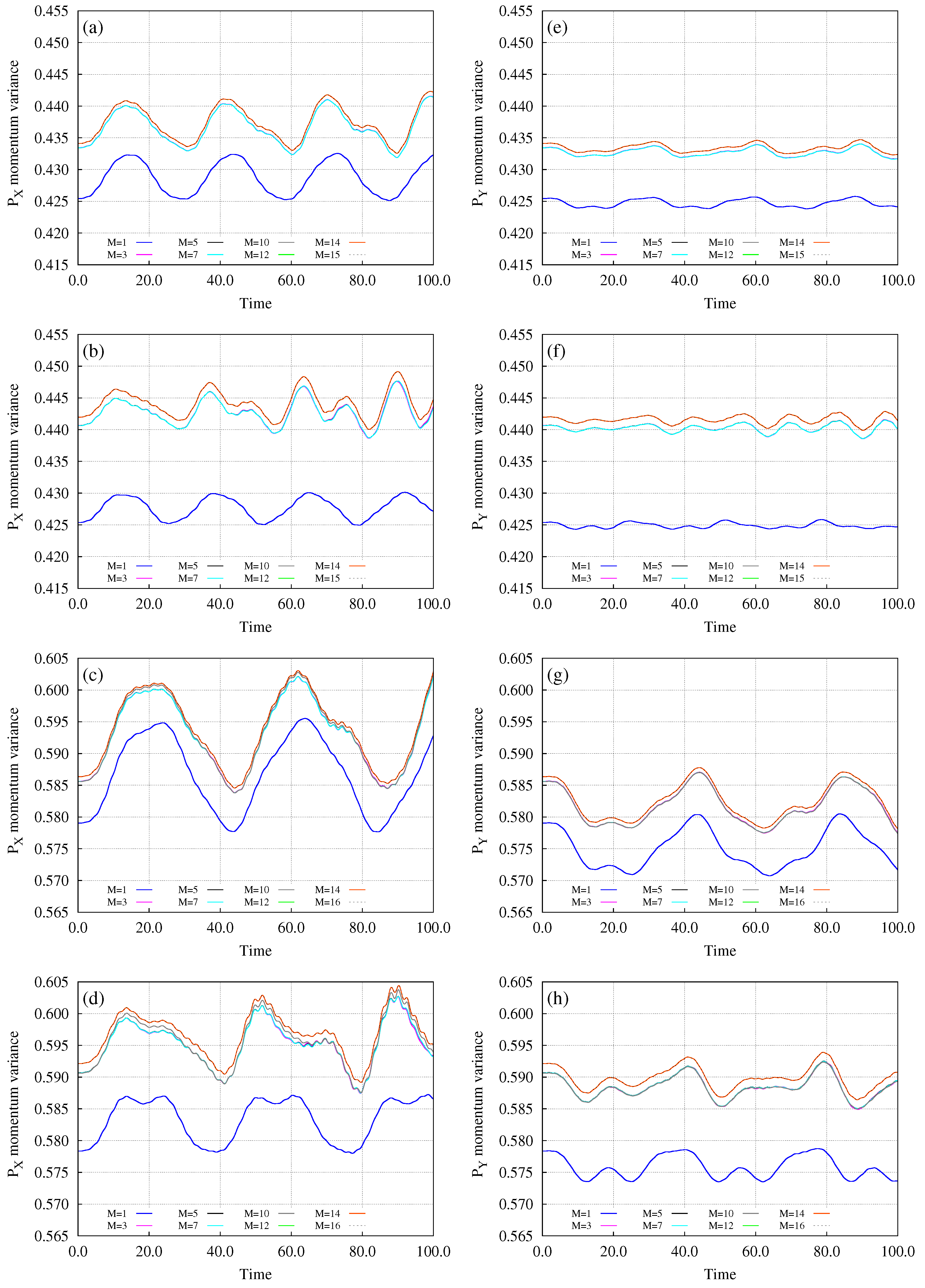
Figure 5.
Angular-momentum variance dynamics following a potential quench. The mean-field ( time-adaptive orbitals) and many-body (using , 5, 7, 10, 12, 14, and 15, 16 time-adaptive orbitals) time-dependent angular-momentum variance per particle, , of bosons in the annuli with barrier heights and interaction strengths (a) , ; (b) , ; (c) , ; and (d) , following a sudden potential tilt by . The respective depletions are plotted in Figure 2. See the text for more details. The quantities shown are dimensionless.
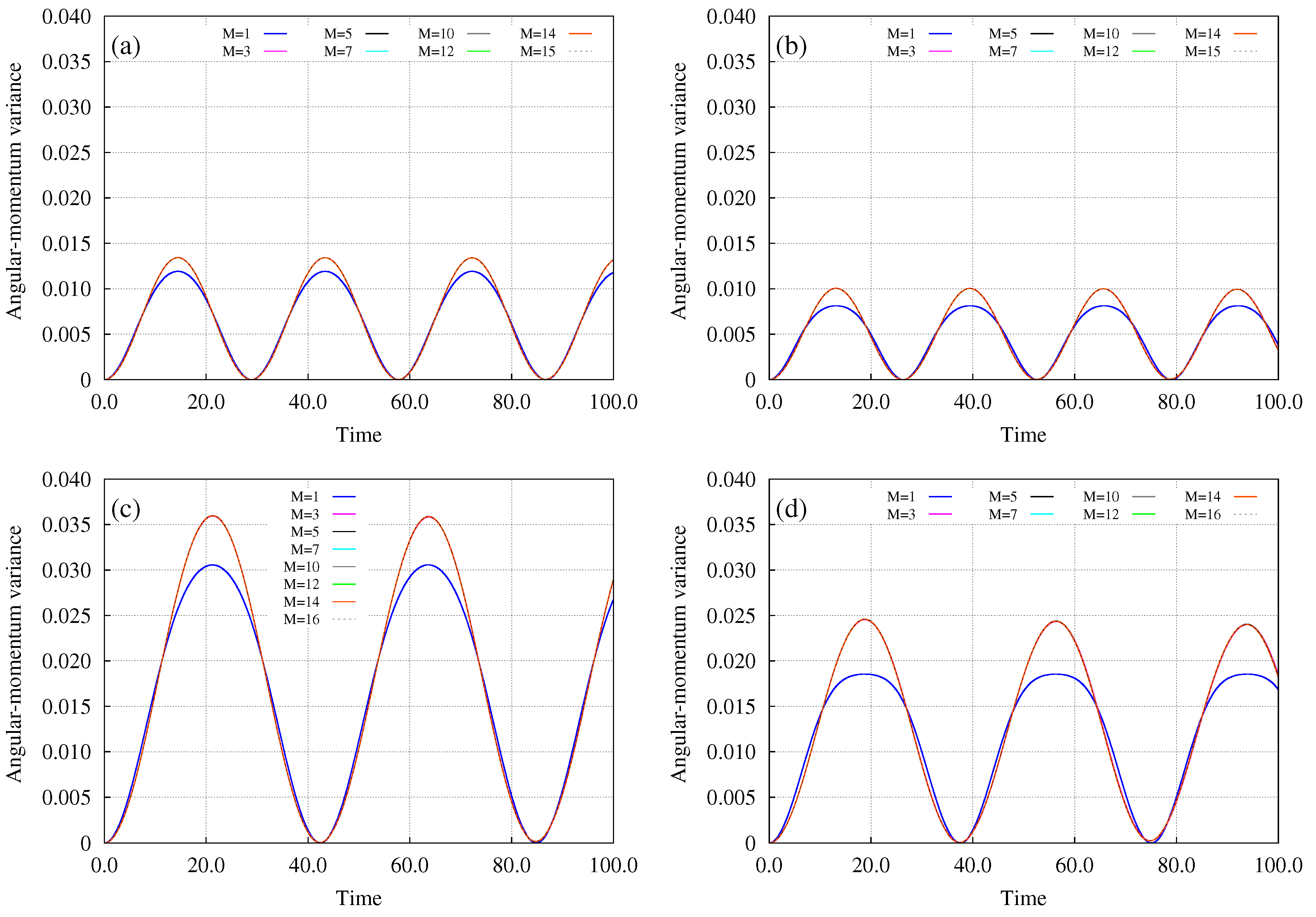
Figure 6.
Depletion dynamics following a potential quench en route to the particle limit. The time-dependent total number of depleted particles, , of , , and bosons with interaction parameter for an annulus with barrier height following a sudden potential tilt by . The number of time-adaptive orbitals is . The respective position, momentum, and angular-momentum variances along with the expectation value of the center-of-mass are plotted in Figure 7. See the text for more details. The quantities shown are dimensionless.
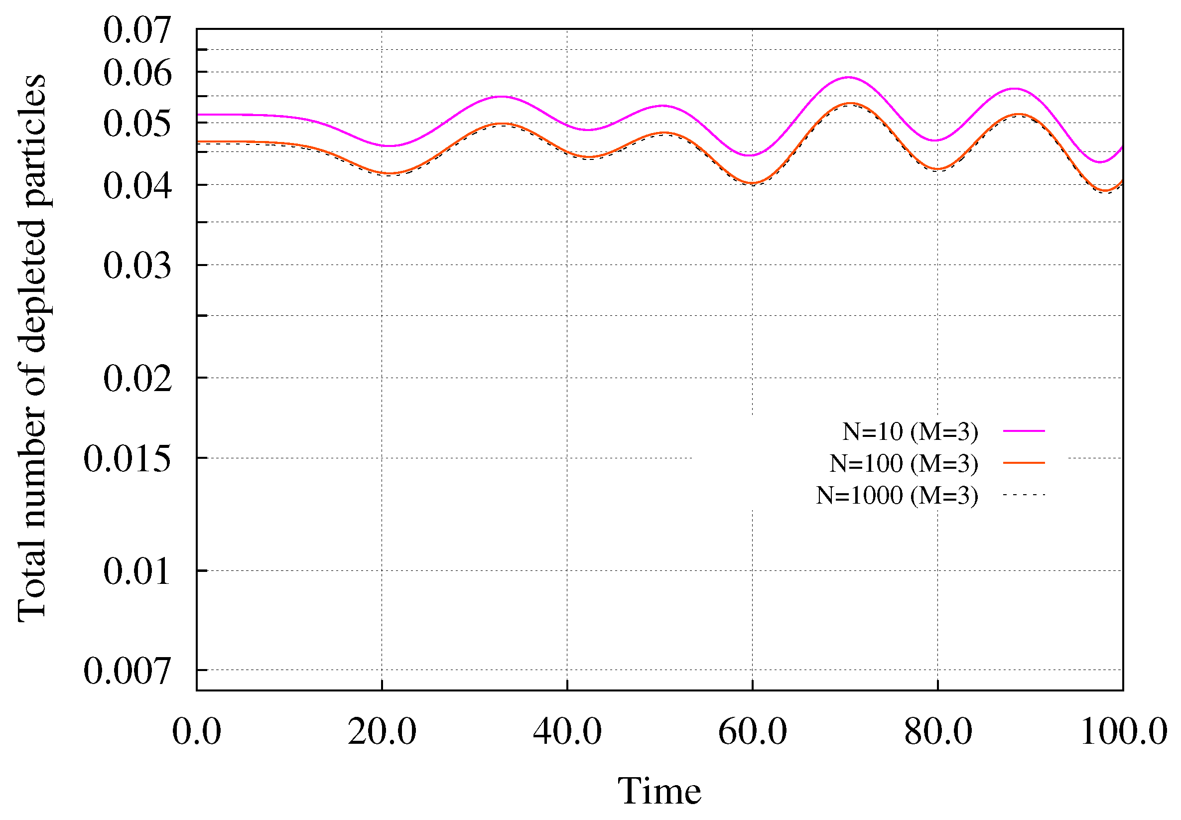
Figure 7.
Position, momentum, and angular-momentum variance dynamics following a potential quench en route to the particle limit. The mean-field ( time-adaptive orbitals) and many-body (using time-adaptive orbitals) time-dependent position variances per particle, (a) and (b) , momentum variances per particle, (c) and (d) , and angular-momentum variance per particle, (f) , of , , and bosons with interaction parameter for an annulus with barrier height following a sudden potential tilt by . (e) The time-dependent expectation value of the center-of-mass, . The respective depletions are plotted in Figure 6. See the text for more details. The quantities shown are dimensionless.

© 2019 by the author. Licensee MDPI, Basel, Switzerland. This article is an open access article distributed under the terms and conditions of the Creative Commons Attribution (CC BY) license (http://creativecommons.org/licenses/by/4.0/).
Share and Cite
MDPI and ACS Style
Alon, O.E. Analysis of a Trapped Bose–Einstein Condensate in Terms of Position, Momentum, and Angular-Momentum Variance. Symmetry 2019, 11, 1344. https://doi.org/10.3390/sym11111344
AMA Style
Alon OE. Analysis of a Trapped Bose–Einstein Condensate in Terms of Position, Momentum, and Angular-Momentum Variance. Symmetry. 2019; 11(11):1344. https://doi.org/10.3390/sym11111344
Chicago/Turabian StyleAlon, Ofir E. 2019. "Analysis of a Trapped Bose–Einstein Condensate in Terms of Position, Momentum, and Angular-Momentum Variance" Symmetry 11, no. 11: 1344. https://doi.org/10.3390/sym11111344
Note that from the first issue of 2016, this journal uses article numbers instead of page numbers. See further details here.