Diagonally Implicit Block Backward Differentiation Formula with Optimal Stability Properties for Stiff Ordinary Differential Equations

Abstract

This paper aims to select the best value of the parameter $\rho$ from a general set of linear multistep formulae which have the potential for efficient implementation. The $\rho$-Diagonally Implicit Block Backward Differentiation Formula ($\rho$-DIBBDF) was proposed to approximate the solution for stiff Ordinary Differential Equations (ODEs) to achieve the research objective. The selection of $\rho$ for optimal stability properties in terms of zero stability, absolute stability, error constant and convergence are discussed. In the diagonally implicit formula that uses a lower triangular matrix with identical diagonal entries, allowing a maximum of one lower-upper (LU) decomposition per integration stage to be performed will result in substantial computing benefits to the user. The numerical results and plots of accuracy indicate that the $\rho$-DIBBDF method performs better than the existing fully and diagonally Block Backward Differentiation Formula (BBDF) methods.

1. Introduction

In many mathematical models of real-world problems, Initial Value Problems (IVPs) involving systems of Ordinary Differential Equations (ODEs) exhibit a phenomenon called stiffness. This phenomenon frequently arises in the study of vibrations, chemical engineering, electrical circuits and control theory. Throughout the history of the development of numerical methods for stiff ODEs, considerable attention has been given to creating a robust algorithm with optimal stability properties. This has led us to design an efficient method that possesses a small error constant, zero stability and a large stability region. Such approaches have been taken by numerous researchers, such as [1,2,3,4,5,6,7].

In this article, we consider the IVPs for first order ODEs of the form

$$y^{\prime }=f(x,y),$$

(1)

with $y\left(a\right)=y_0$ in the interval of $a\le x\le b$. The system (1) is said to be linear with constant coefficients if $f(x,y)=Ay+\mathsf{\Phi }\left(x\right)$, where A is an $m\times m$ constant matrix, while y, f and $\mathsf{\Phi }\left(x\right)$ are m-dimensional vectors. The matrix A has distinct eigenvalues, ${\lambda }_i$ and corresponding eigenvectors, $c_i$, where $i=1,2,\dots ,m$ . The system of ODEs has a general solution in the form of

$$y\left(x\right)=\sum _{i=0}^m{k}_i{e}^{{\lambda }_{i}x}{c}_i+\mathsf{\Psi }\left(x\right).$$

According to the definition provided in [8], (1) is considered stiff if the eigenvalues ${\lambda }_i$ of ${\displaystyle \frac{\partial f}{\partial y}}$ satisfy the following conditions:

(i) 

$Re\left({\lambda }_i\right)<0$ and

(ii) 

$\underset{i}{max}|Re\left({\lambda }_i\right)|\gg \underset{i}{min}\left|Re\left({\lambda }_i\right)\right|$ where the ratio $\frac{\underset{i}{max}|Re\left({\lambda }_i\right)}{\underset{i}{min}\left|Re\left({\lambda }_i\right)\right|}$ is called the stiffness ratio or stiffness index.

For a non-linear system, (1) is stiff in an interval I of x if, for $x\in I,$ the eigenvalues ${\lambda }_i\left(x\right)$ satisfy (i) and (ii) above.

According to [8], stiffness requires solving the implicit equations by using Newton iteration, which in turn demands an evaluation of the Jacobian at each step. These requirements will increase the computational time and therefore, is not cost-efficient for the users. Because of the high cost of evaluating the stages in a fully implicit method, [9] reported that many researchers have opted to reduce it to a diagonally implicit method. Prior works along this line were discussed by [10,11,12,13,14].

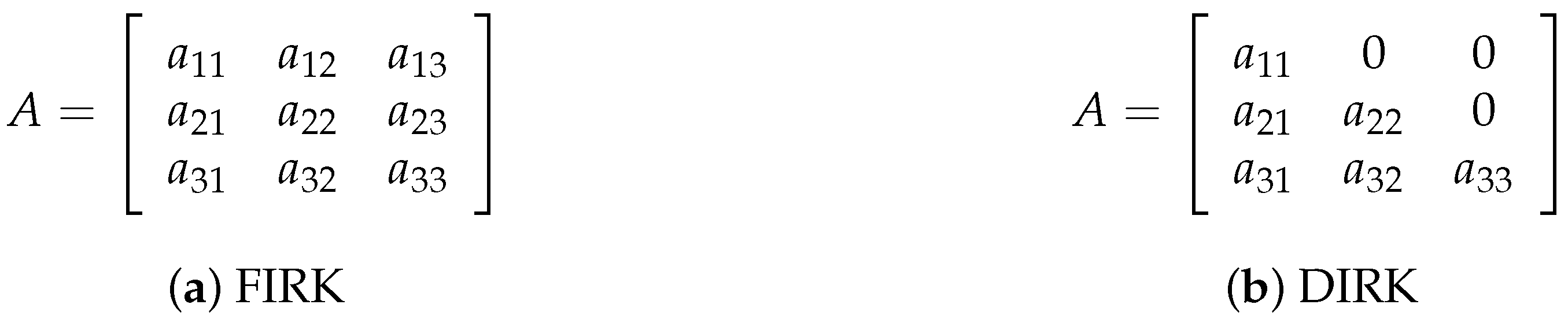
In practical applications involving stiff ODEs, the Diagonally Implicit Runge–Kutta (DIRK) class is the most often used among the Implicit Runge–Kutta (IRK) methods. Figure 1 illustrates the fully implicit and diagonally implicit classes of Runge–Kutta (RK) methods, which can be defined as a 3 × 3 matrix. As stated in [15], RK methods are characterized by excellent stability properties that make them useful for solving stiff ODEs systems. However, for a Fully Implicit Runge–Kutta (FIRK) method, a system of $n\times r$ non-linear equations must be solved in each of its integration stage, where n is the dimension of the problem and r is the number of stages, as described by [16]. Thus, the authors of [17,18] proposed a DIRK method that uses a lower triangular matrix, A with $a_{ij}=0$ for $i<j$. It implies that the DIRK technique needs to solve a series of r-implicit structures for each n instead of an $n\times r$ system as in the FIRK method. This structure permits solving each stage of the system separately instead of solving all the stages simultaneously. Another common requirement, as stated in [19], is for the non-zero diagonal entries of A to be identical, allowing for a maximum of one lower-upper (LU) decomposition per integration stage.

The well-known Backward Differentiation Formula (BDF) has been the technique of choice for the numerical solution of stiff differential equations for many years. The classical BDF method approximates the solution for $y_{n+1}$ at $x_{n+1}$ point in every step. Ibrahim et al. in [20] introduced the Block Backward Differentiation Formula (BBDF) method to reduce the number of integration steps and the computational time of existing numerical integrator while maintaining the accuracy. Many attempts have been made to implement the BBDF method in solving stiff problems because it has been proven as more accurate and efficient than the non-block method (see [20,21,22]) and existing solvers (see [23,24]).

Motivated by the fact that the existing works carried out based on RK and BBDF are suitable for solving stiff ODEs, we aim to formulate an efficient BBDF method in a diagonally implicit form that is expected to be faster than the fully implicit methods in the existing literature.

This paper is organized as follows. The derivation of the method is presented in Section 2. In Section 3, we discuss the stability properties of the method encompassing zero stability, absolute stability, order of the method and convergence. Next, the implementation of the derived method using Newton iteration is discussed in Section 4, followed by the numerical results for the proposed and existing methods in Section 5. Finally, the conclusions are provided in Section 6.

2. The $\mathbf{\rho }$-Diagonally Implicit Block Backward Differentiation Formula

Various methods can be used to compute the approximate solution of $y\left(x\right)$. One of these methods is the general linear k-step method in the form of

$$\sum _{j=0}^k{\alpha }_j{y}_{n+j}=h\sum _{j=0}^k{\beta }_j{f}_{n+j}.$$

(2)

If ${\beta }_0={\beta }_1=\dots ={\beta }_{k-1}=0$ and ${\beta }_k\ne 0$, (2) becomes a BDF as outlined by Gear in [25] in the form of

$$\sum _{j=0}^k{\alpha }_j{y}_{n+j}=h{\beta }_k{f}_{n+k}.$$

(3)

Vijitha-Kumara in [26] modified the formula in (3) by taking an arbitrary ${\beta }_{k-1}\ne 0$, introducing the free parameter $\rho$ and formulating the non-block Fixed Step Formula (FSF) of

$$\sum _{j=0}^k{\alpha }_j{y}_{n+j}=h{\beta }_k\left(f_{n+k}-\rho f_{n+k-1}\right),$$

(4)

where ${\beta }_{k-1}=\rho {\beta }_k$.

The definition of the k-step 2-point block linear multistep method (LMM) of BBDF as given by Ibrahim et al. in [20] is in the form of

$$\sum _{j=0}^k{A}_{j,i}{y}_{n+j}=h\sum _{j=0}^k{B}_{j,i}{f}_{n+j},$$

(5)

where $k=i=1,2$ for $y_{n+1}$ and $y_{n+2}$ respectively; $A_{k,i}=1$; $A_{j,i},B_{j,i}$ are $r\times r$ coefficient matrices; $f_{n+j}=f(x_{n+j},y_{n+j})$ and h = step size used. This constant step size method is implemented by approximating $y_{n+1},\dots ,y_{n+j}$ concurrently in a block at the time discretization points of $x_{n+1},\dots ,x_{n+j}$.

In this section, we will derive the $\rho$-Diagonally Implicit Block Backward Differentiation Formula ($\rho$-DIBBDF) based on the derivation of BBDF by Ibrahim et al. in [20] and FSF by Vijitha-Kumara in [26]. FSF is a non-block method, where the computation proceeds to an approximation of $y_{n+1}$ at the $x_{n+1}$ one step at a time. To increase the efficiency of the classical approach, we proposed a method that constructed in a block, where the solutions of $y_{n+1}$ and $y_{n+2}$ were approximated concurrently in a block by using three back values at the points $x_n,x_{n-1}$ and $x_{n-2}$ of the previous block. The development of our method involves the hybrid-like process of implementing the FSF and BBDF, which produce as many A-stable formulae as possible. Suleiman et al. [22] extended the formula in (5), implemented the strategy in [26] by adding extra future points and proposed the 2-point Superclass of BBDF (2SBBDF). The BBDF and 2SBBDF are formulated in a fully implicit manner. We are motivated to develop the $\rho$-DIBBDF to enhance the efficiency of the fully implicit BBDF method by proposing a diagonally implicit method that requires fewer computations of the differentiation coefficients, thus minimizing the cumulative error (refer to [10]). Our proposed method differs from the Diagonally Implicit 2-point BBDF (DI2BBDF) in [10], which provides a fixed formula for each point and order because our method generates a different set of formulae depending on the free parameter chosen in an attempt to achieve the optimal stability properties and accurate numerical results.

The $\rho$-DIBBDF method takes the general form of

$$\sum _{j=0}^{k+2}{\alpha }_{j-2,k}{y}_{n+j-2}=h{\beta }_{k,k}\left(f_{n+k}-\rho f_{n+k-1}\right),k=1,2$$

(6)

where ${\beta }_{k-1,k}=\rho {\beta }_{k,k}$. The linear difference operator $L_i$ associated with the formula in (6), is defined as

$$L\left[y\left(x_n\right);h\right]=\sum _{j=0}^{k+2}{\alpha }_{j-2,k}{y}_{n+j-2}-h{\beta }_{j,k}(y_{n+k}^{\prime }-\rho y_{n+k-1}^{\prime }).$$

(7)

Expanding $y_{n+j-2}$ and its derivative by using the Taylor series method and collecting the common terms of the derivative y in (7) gives

$$L\left[y\left(x_n\right);h\right]=C_{0}y\left(x\right)+C_{1}h{y}^{\prime }\left(x\right)+\dots +C_q{h}^q{y}^{\left(q\right)}\left(x\right).$$

(8)

The general form of the constant $C_q$ is given by

$$\begin{array}{cc}\hfill C_0& =\sum _{j=0}^{k+2}{\alpha }_{j-2,k},\hfill \\ \hfill C_1& =\sum _{j=0}^{k+2}\frac{{(j-2)}^1}{1!}{\alpha }_{j-2,k}-\frac{k^{\left(0\right)}}{0!}{\beta }_{j,k}+\rho {\beta }_{j,k},\hfill \\ \hfill ⋮& \\ \hfill C_q& =\sum _{j=0}^{k+2}\frac{{(j-2)}^q}{q!}{\alpha }_{j-2,k}-\frac{k^{(q-1)}}{(q-1)!}{\beta }_{j,k}+\frac{{(k-1)}^{(q-1)}}{(q-1)!}\rho {\beta }_{j,k},q=2,3,\dots \hfill \end{array}$$

(9)

The values of $k=1,2$ in (6) indicate the first and second points, respectively. By setting ${\alpha }_{1,1}=1$, ${\alpha }_{2,2}=1$, ${\alpha }_{0,2}=0$ and solving (9) simultaneously, we obtain the following coefficients of ${\alpha }_{j-2,k}$ and ${\beta }_{j,k}$ in terms of $\rho$ as listed in

Table 1. List of coefficients for $\rho$-DIBBDF.

k	${\mathit{\alpha }}_{-2,\mathit{k}}$	${\mathit{\alpha }}_{-1,\mathit{k}}$	${\mathit{\alpha }}_{0,\mathit{k}}$	${\mathit{\alpha }}_{1,\mathit{k}}$	${\mathit{\alpha }}_{2,\mathit{k}}$	${\mathit{\beta }}_{0,\mathit{k}}$	${\mathit{\beta }}_{1,\mathit{k}}$	${\mathit{\beta }}_{2,\mathit{k}}$
1	${\displaystyle \frac{\rho +2}{2\rho -11}}$	${\displaystyle \frac{-3\left(2\rho +3\right)}{2\rho -11}}$	${\displaystyle \frac{3\left(\rho +6\right)}{2\rho -11}}$	1	0	${\displaystyle \frac{-6\rho }{2\rho -11}}$	${\displaystyle \frac{-6}{2\rho -11}}$	0
2	${\displaystyle \frac{2\rho +3}{6\rho -19}}$	${\displaystyle \frac{-2\left(3\rho +4\right)}{6\rho -19}}$	0	${\displaystyle \frac{-2\left(\rho -12\right)}{6\rho -19}}$	1	0	${\displaystyle \frac{-12\rho }{6\rho -19}}$	${\displaystyle \frac{-12}{6\rho -19}}$

:

Substituting the coefficients obtained in Table 1 into (6) gives the following general corrector formula for the 2-point $\rho$-DIBBDF:

$$\begin{array}{cc}\hfill y_{n+1}& =-\frac{\rho +2}{2\rho -11}{y}_{n-2}+\frac{3\left(2\rho +3\right)}{2\rho -11}{y}_{n-1}-\frac{3\left(\rho +6\right)}{2\rho -11}{y}_n+\frac{6\rho }{2\rho -11}h{f}_n-\frac{6}{2\rho -11}h{f}_{n+1},\hfill \\ \hfill y_{n+2}& =-\frac{2\rho +3}{6\rho -19}{y}_{n-2}+\frac{2\left(3\rho +4\right)}{6\rho -19}{y}_{n-1}+\frac{2\left(\rho -12\right)}{6\rho -19}{y}_{n+1}+\frac{12\rho }{6\rho -19}h{f}_{n+1}-\frac{12}{6\rho -19}h{f}_{n+2}.\hfill \end{array}$$

(10)

The matrix form of the corrector formula in (10) is therefore represented by

$$\begin{array}{c}\begin{array}{cc}\hfill \left[\begin{array}{cc}1& 0\\ -\frac{2\left(\rho -12\right)}{6\rho -19}& 1\end{array}\right]\left[\begin{array}{c}{y}_{n+1}\\ y_{n+2}\end{array}\right]& =\left[\begin{array}{cc}0& -\frac{\rho +2}{2\rho -11}\\ 0& -\frac{2\rho +3}{6\rho -19}\end{array}\right]\left[\begin{array}{c}{y}_{n-3}\\ y_{n-2}\end{array}\right]+\left[\begin{array}{cc}\frac{3\left(2\rho +3\right)}{2\rho -11}& -\frac{3\left(\rho +6\right)}{2\rho -11}\\ \frac{2\left(3\rho +4\right)}{6\rho -19}& 0\end{array}\right]\left[\begin{array}{c}{y}_{n-1}\\ y_n\end{array}\right]\hfill \\ & +h\left[\begin{array}{cc}0& \frac{6\rho }{2\rho -11}\\ 0& 0\end{array}\right]\left[\begin{array}{c}{f}_{n-1}\\ f_n\end{array}\right]+h\left[\begin{array}{cc}-\frac{6}{2\rho -11}& 0\\ \frac{12\rho }{6\rho -19}& -\frac{12}{6\rho -19}\end{array}\right]\left[\begin{array}{c}{f}_{n+1}\\ f_{n+2}\end{array}\right].\hfill \end{array}\end{array}$$

(11)

3. Selection of Parameter $\mathbf{\rho }$

To determine whether the numerical method can provide acceptable results, we need to investigate the stability of the method. In this section, the practical efficiency of the numerical method concerning three essential concepts, namely zero stability, absolute stability and convergence will be studied. According to Dahlquist in [27], a potentially useful numerical method for solving stiff ODE systems must have good accuracy and a reasonably large region of absolute stability. In designing an efficient method, authors in [2,3,7] considered developing methods with smaller error constants. The development of our method closely follows the works of [22,26] but in the DI scheme. To overcome the setback in choosing the best $\rho$ as reported in [28], we will choose a better value for $\rho$ with optimal stability properties that will give better accuracy to the approximate solution. The parameter $\rho$ is restricted to $(-1,1)$ so that the underlying $\rho$-DIBBDF in (6) satisfies the necessary condition for stiff stability. The relevant proof for $y_{n+1}$ is provided in this section concerning the theorem due to [29] (refer to [26]). The proof of the second point is straightforward by adopting an approach similar to that of the first point.

To begin with, the associate $\varrho$ and $\sigma$ polynomials of (6) are given as follows

$$\begin{array}{cc}\hfill \varrho \left(\xi \right)& ={\xi }^3+{\alpha }_{0,k}{\xi }^2+{\alpha }_{-1,k}\xi +{\alpha }_{-2,k},\hfill \\ \hfill \sigma \left(\xi \right)& ={\beta }_{k,k}\left({\xi }^3-\rho {\xi }^2\right).\hfill \end{array}$$

Then, by using the following polynomials of $r\left(z\right)$ and $s\left(z\right)$,

$$\begin{array}{cc}\hfill r\left(z\right)& ={\left(\frac{1-z}{2}\right)}^3\varrho \left(\frac{1+z}{1-z}\right),\hfill \\ \hfill s\left(z\right)& ={\left(\frac{1-z}{2}\right)}^3\sigma \left(\frac{1+z}{1-z}\right),\hfill \end{array}$$

we define $P(z,\mu )=r\left(z\right)-\mu s\left(z\right)$ where $\mu =h\lambda$. $P(z,\mu )$ can be simplified as

$$-\left(2\rho -11\right)P(z,\mu )=a_3{z}^3+a_2{z}^2+a_{1}z+a_0,$$

(12)

where

$$\begin{array}{cc}\hfill a_0& =6(\rho -1)\mu ,\hfill \\ \hfill a_1& =-12(\rho -1)+6(\rho -3)\mu ,\hfill \\ \hfill a_2& =-12(\rho -3)-6(\rho +3)\mu ,\hfill \\ \hfill a_3& =8(\rho +5)-6(\rho +1)\mu .\hfill \end{array}$$

(13)

The following lemma will be used in the next theorem.

Lemma 1.

Let $p\left(x\right)=a_3{x}^3+a_2{x}^2+a_{1}x+a_0$, where $a_i$ are real numbers and $a_3\ne 0$. Then $p\left(x\right)$ is a Hurwitz polynomial if and only if the conditions (i) and (ii) both hold.

(i) 

$a_{i}are either all positive or negative$,

(ii) 

$a_1{a}_2-a_0{a}_3>0.$

Proof. 

See [30]. □

According to [26], (6) is $A_0$-stable if and only if its corresponding $P(z,\mu )$ is a Hurwitz polynomial for all $\mu <0$.

Theorem 1.

The method is $A_0$-stable for all ρ in $(-1,1)$ .

Proof. 

Clearly from (13), $a_i>0$, where $i=0,1,2,3$ for all $\mu <0$ and $\rho \in (-1,1)$. For (ii), $a_1{a}_2-a_0{a}_3$ can be written as $144(\rho -1)(\rho -3)-48({\rho }^2-8\rho +13)\mu +288{\mu }^2$. Thus, $a_1{a}_2-a_0{a}_3>0$ for all $\mu <0$ and $\rho \in (-1,1)$. By Lemma 1, $-\left(2\rho -11\right)P(z,\mu )$ in (12) is a Hurwitz polynomial and so is $P(z,\mu )$ for all $\mu <0$ and $\rho \in (-1,1)$. □

The following theorem due to [31] gives necessary and sufficient conditions for stiff stability.

Theorem 2.

The conditions (i)–(iv) are necessary and sufficient for a convergent method to be stiffly stable.

(i) 

The method is $A_0$-stable,

(ii) 

The modulus of any root of the polynomial $\frac{\varrho \left(\xi \right)}{\xi -1}$ is less than 1,

(iii) 

The roots of $\sigma \left(\xi \right)$ of modulus 1 are simple,

(iv) 

If ${\xi }_0$ is a root of $\sigma \left(\xi \right)$ with $|{\xi }_0|=1$, then $\frac{\varrho \left(\xi \right)}{\xi {\sigma }^{\prime }\left(\xi \right)}$ at $\xi ={\xi }_0$ is real and positive.

The following lemma will be used to prove the next theorem.

Lemma 2.

Let $p\left(x\right)=a_2{x}^2+a_{1}x+a_0$, where $a_0,a_1,a_2\ne 0$ and $a_0,a_1,a_2$ are real. Then $p\left(x\right)$ is a Schur polynomial if and only if the conditions of (i) and (ii) are met.

(i) 

|a₀| < |a₂| ,

(ii) 

|a₁| < |a₂ + a₀| .

Proof. 

See [26]. □

Theorem 3.

The method is strongly stable for $\rho \in (-1,1)$.

Proof. 

It suffices to show that $\frac{\varrho \left(\xi \right)}{\xi -1}$ is a Schur polynomial for $\rho \in (-1,1)$. From Table 1, ${\alpha }_{-2,1}+{\alpha }_{-1,1}+{\alpha }_{0,1}+1=0$, $\varrho \left(\xi \right)$ can be simplified as $\varrho \left(\xi \right)=(\xi -1)(a_2{x}^2+a_{1}x+a_0)$, where $a_0=-{\alpha }_{-2,1}=-\frac{\rho +2}{2\rho -11},a_1=-({\alpha }_{-2,1}+{\alpha }_{-1,1})=-\left(\frac{-5\rho -7}{2\rho -11}\right)$ and $a_2=1$. Since $-\frac{\rho +2}{2\rho -11}\le \frac{1}{3}$ for $-1<\rho <1$, we have $a_0<a_2$. Now, $a_2+a_0=\frac{\rho -13}{2\rho -11}$ and $|a_2+a_0|-|a_1|=\frac{6(\rho -1)}{2\rho -11}>0$ for $-1<\rho <1$. Thus, by Lemma 2, $\frac{\varrho \left(\xi \right)}{\xi -1}$ is a Schur polynomial. □

Theorem 4.

The method is stiffly stable for $\rho \in (-1,1)$.

Proof. 

$\sigma \left(\xi \right)={\beta }_{1,1}\left({\xi }^3-\rho {\xi }^2\right)$ where ${\beta }_{1,1}=\frac{-6}{2\rho -11}$. The roots of $\sigma \left(\xi \right)$ are $0,\rho$ and it has simple root of modulus 1 when $\rho =-1$. Now Theorem 2 together with Theorem 1 and Theorem 3 imply that the method is stiffly stable for all $\rho \in (-1,1)$. □

Corollary 1.

The method is $A\left(\alpha \right)$-stable for all $\rho \in (-1,1)$.

Proof. 

Stiff stability implies $A\left(\alpha \right)$-stability (refer to [31]). □

For the order 3 method, the intensive work done by [26] shows that $\rho =-0.75$ will produce accurate numerical results with optimal stability properties. The stability analysis of the proposed method for $\rho =-0.75$ will be presented in the following subsections.

3.1. Zero Stability

Zero stability is one of the important forms of stability for the numerical solution of IVPs. It is defined by [32] as:

Definition 1.

The method in (10) is said to have zero stability if no root of its characteristic polynomial has a modulus higher than one and if any root with a modulus of one is simple.

Consider the scalar test equation $y^{\prime }=\lambda y$. Substitute $h\lambda =\overline{h}$ into (11) and rewrite it in the matrix form to get

$$\begin{array}{c}\begin{array}{cc}\hfill \left[\begin{array}{cc}1+\frac{6}{2\rho -11}\overline{h}& 0\\ -\frac{2\left(\rho -12\right)}{6\rho -19}-\frac{12\rho }{6\rho -19}\overline{h}& 1+\frac{12}{6\rho -19}\overline{h}\end{array}\right]\left[\begin{array}{c}{y}_{n+1}\\ y_{n+2}\end{array}\right]& =\left[\begin{array}{cc}\frac{3\left(2\rho +3\right)}{2\rho -11}& -\frac{3\left(\rho +6\right)}{2\rho -11}+\frac{6\rho }{2\rho -11}\overline{h}\\ \frac{2\left(3\rho +4\right)}{6\rho -19}& 0\end{array}\right]\left[\begin{array}{c}{y}_{n-1}\\ y_n\end{array}\right]\hfill \\ & +\left[\begin{array}{cc}0& -\frac{\rho +2}{2\rho -11}\\ 0& -\frac{2\rho +3}{6\rho -19}\end{array}\right]\left[\begin{array}{c}{y}_{n-3}\\ y_{n-2}\end{array}\right]\hfill \end{array}\end{array}$$

(14)

which is equivalent to $A_0{Y}_m=B_0{Y}_{m-1}+C_0{Y}_{m-2}$. By inserting the coefficients of $A_0,B_0$ and $C_0$ in (14) into the determinant formula viz. $|A_0{t}^2-B_{0}t-C_0|$, we obtain the following stability polynomial in terms of $\rho$:

$$\begin{array}{cc}\hfill R(t,\overline{h})& =\left[\frac{-1}{(2\rho -11)(6\rho -19)}\right]72{\overline{h}}^2{\rho }^2{t}^3-72{\overline{h}}^2{t}^4-24\overline{h}{\rho }^2{t}^3-60\overline{h}\rho t^4-12{\rho }^2{t}^4+24\overline{h}{\rho }^2{t}^2-288\overline{h}\rho t^3\hfill \\ & +246\overline{h}{t}^4+30{\rho }^2{t}^3+104\rho t^4+12\overline{h}\rho t^2+108\overline{h}{t}^3-24{\rho }^2{t}^2-24\rho t^3-209t^4-18\overline{h}{t}^2+6{\rho }^{2}t\hfill \\ & -96\rho t^2+261t^3+16\rho t-63t^2+11t=0.\hfill \end{array}$$

(15)

By plugging $\overline{h}=0$ and solving (15) with respect to t, we obtain the roots, t as listed in (16).

$$\begin{array}{c}\begin{array}{cc}\hfill t& =0,1,\frac{1}{12{\rho }^2-104\rho +209}\left(9{\rho }^2+\sqrt{9{\rho }^4+1152{\rho }^3+2346{\rho }^2-120\rho -1623}+40\rho +26\right),\hfill \\ & -\frac{1}{12{\rho }^2-104\rho +209}\left(-9{\rho }^2+\sqrt{9{\rho }^4+1152{\rho }^3+2346{\rho }^2-120\rho -1623}-40\rho -26\right).\hfill \end{array}\end{array}$$

(16)

By setting $\rho =-0.75$, we obtain the roots, $t=0,1,0.003617\pm 0.08982i$. Since the roots of the stability polynomial for $\rho =-0.75$ satisfy Definition 1, we conclude that the method is said to be zero stable.

3.2. Absolute Stability

According to [32], if the employed method has a region of absolute stability that includes the entire negative-plane, then there will be no constraint on the step length imposed by the stability.

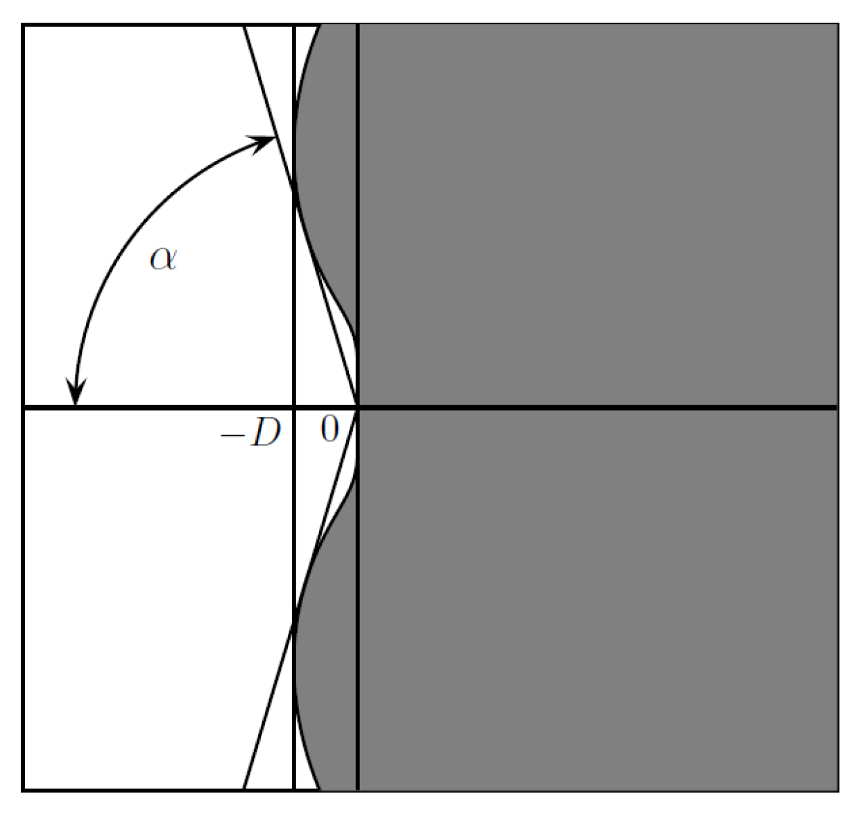
Definition 2.

A numerical method is said to be A-stable if ${\Re }_A\supseteq \{h\lambda \mid Re\left(h\lambda \right)<0\}$.

However, the A-stability requirement places a severe restriction on selecting appropriate LMMs. This restriction is known as Dahlquist’s second barrier, which states that the order of an A-stable LMM must be $\le 2$ (see [27]). This demanding requirement motivates the following definition by [33]:

Definition 3.

A numerical method is said to be $A\left(\alpha \right)$-stable, $\alpha \in \left(0,\pi /2\right)$ if ${\Re }_A\supseteq \{h\lambda \mid -\alpha <\pi -arg\left(h\lambda \right)<\alpha \}$ as shown in Figure 2.

The boundary of the stability region is determined by putting $t=e^{i\theta }$ in (15) where $0\le \theta \le 2\pi$ for which $\left|t\right|<1$. The stable region is located outside the boundary of the solid line and the unstable region is within the enclosed area. The absolute stability region of our method for $\rho =-0.75$ is plotted in a complex $h\lambda$ plane and shown below.

Referring to Figure 3, we can observe that almost the whole left-plane of the circle lies within a stable region and hence, based on Definition 3, the method is considered $A\left(\alpha \right)$-stable.

3.3. Order of the Method and Error Constant

The definition of the order of the method given by [8] is provided in Definition 4, as follows:

Definition 4.

The linear multistep method (5) and the associated difference operator, $L_i$ as defined by (6), are said to be of order p if in (8), $C_0=C_1=\dots =C_p=0$ and $C_{p+1}\ne 0$, where $C_{p+1}$ is the error constant.

The error constant of the method can be obtained by substituting the corresponding values of ${\alpha }_{j,k}$ and ${\beta }_{j,k}$ in Table 1 into (9), which gives

$$\begin{array}{cc}\hfill C_0& =\sum _{j=0}^4{\alpha }_{j,k}=\left[\begin{array}{c}0\\ 0\end{array}\right],\hfill \\ \hfill C_1& =\sum _{j=0}^4\frac{j}{1!}{\alpha }_{j,k}-{\beta }_{j,k}=\left[\begin{array}{c}0\\ 0\end{array}\right],\hfill \\ \hfill C_2& =\sum _{j=0}^4\frac{j^2}{2!}{\alpha }_{j,k}-\frac{j}{1!}{\beta }_{j,k}=\left[\begin{array}{c}0\\ 0\end{array}\right],\hfill \\ \hfill C_3& =\sum _{j=0}^4\frac{j^3}{3!}{\alpha }_{j,k}-\frac{j^2}{2!}{\beta }_{j,k}=\left[\begin{array}{c}0\\ 0\end{array}\right],\hfill \\ \hfill C_4& =\sum _{j=0}^4\frac{j^4}{4!}{\alpha }_{j,k}-\frac{j^3}{3!}{\beta }_{j,k}=\left[\begin{array}{c}\frac{1}{2}\frac{\rho +3}{2\rho -11}\\ \frac{3(\rho +2)}{6\rho -19}\end{array}\right]=\left[\begin{array}{c}\frac{-9}{100}\\ \frac{-15}{94}\end{array}\right].\hfill \end{array}$$

(17)

Since $C_4\ne 0$ in (17), following Definition 4, we conclude that the derived method has the order 3 with $\frac{-9}{100}$ and $\frac{-15}{94}$ as the error constants of $y_{n+1}$ and $y_{n+2}$ respectively.

3.4. Convergence

An essential property of an acceptable LMM is that the solution generated by the method converges to an exact solution as the step size approaches zero. A theorem provided by [35] states that a method of an LMM class in (6) is convergent if and only if, it is both consistent and zero stable. The proof for this theorem can be found in [35]. For this theorem to be satisfied, the following consistency conditions given by [8] must be fulfilled:

(a)

${\sum }_{j=0}^{k+2}{\alpha }_{j-2,k}=0,$

(b)

${\sum }_{j=0}^{k+2}j{\alpha }_{j-2,k}={\sum }_{j=0}^{k+2}{\beta }_{j,k}.$

By applying the above consistency conditions for the respective coefficients of $y_{n+1}$ and $y_{n+2}$ in Table 1, we obtained:

$$\begin{array}{c}a)\sum _{j=0}^{k+2}{\alpha }_{j-2,k}=\left[\begin{array}{c}\frac{\rho +2}{2\rho -11}\\ \frac{2\rho +3}{6\rho -19}\end{array}\right]+\left[\begin{array}{c}\frac{-3\left(2\rho +3\right)}{2\rho -11}\\ \frac{-2\left(3\rho +4\right)}{6\rho -19}\end{array}\right]+\left[\begin{array}{c}\frac{3\left(\rho +6\right)}{2\rho -11}\\ 0\end{array}\right]+\left[\begin{array}{c}1\\ \frac{-2\left(\rho -12\right)}{6\rho -19}\end{array}\right]+\left[\begin{array}{c}0\\ 1\end{array}\right]=\left[\begin{array}{c}0\\ 0\end{array}\right],\hfill \\ b)\sum _{j=0}^{k+2}j{\alpha }_{j-2,k}=0\left[\begin{array}{c}\frac{\rho +2}{2\rho -11}\\ \frac{2\rho +3}{6\rho -19}\end{array}\right]+1\left[\begin{array}{c}\frac{-3\left(2\rho +3\right)}{2\rho -11}\\ \frac{-2\left(3\rho +4\right)}{6\rho -19}\end{array}\right]+2\left[\begin{array}{c}\frac{3\left(\rho +6\right)}{2\rho -11}\\ 0\end{array}\right]+3\left[\begin{array}{c}1\\ \frac{-2\left(\rho -12\right)}{6\rho -19}\end{array}\right]+4\left[\begin{array}{c}0\\ 1\end{array}\right]\hfill \\ =\left[\begin{array}{c}\frac{6\rho -6}{2\rho -11}\\ \frac{12\rho -12}{6\rho -19}\end{array}\right]=\left[\begin{array}{c}\frac{21}{25}\\ \frac{42}{47}\end{array}\right]\hfill \\ =\sum _{j=0}^{k+2}{\beta }_{j,k}.\hfill \end{array}$$

Since the method for $\rho =-0.75$ is zero stable as stated in Section 3.1 and both consistency conditions are successfully met, we conclude that the derived method converged.

The $\alpha ,D$ in $A\left(\alpha \right)$-stability and error constants $\left(EC\right)$ of the underlying $\rho$-DIBBDF in (7) for $\rho =-0.75,-0.60,0.50$ and $0.95$ are given in

Table 2. Comparison of stability analysis for $\rho$-DIBBDF, BBDF and DI2BBDF.

$\mathit{\rho }$ or Method	−0.75	−0.60	0.50	0.95	BBDF	DI2BBDF
$\alpha$	$85.{657}^{\circ }$	86.084${}^{\circ }$	$88.{352}^{\circ }$	${90}^{\circ }$	$90.0^{\circ }$	$83.{647}^{\circ }$
D	−0.156	−0.115	−0.016	0	0	−0.226
$\left|EC\right|$$y_{n+1}$	0.0900	0.0984	0.1750	0.2170	0.1667	0.1364
$\left|EC\right|$$y_{n+2}$	0.1596	0.1858	0.4688	0.6654	0.1364	0

. We choose these $\rho$ values to compare with $\rho =-0.75$ to ensure a higher accuracy for the numerical results by selecting the best parameter $(\rho =-0.75),$ as proven for the non-block FSF in [26].

4. Implementation of the Method

In this section, the approximation of $y_{n+1}$ and $y_{n+2}$ values in (14) will be implemented using the Newton’s iteration. Formula in (10) can be represented in the following form:

$$\begin{array}{cc}\hfill y_{n+1}& ={\alpha }_1{y}_{n+2}+{\beta }_{1}h{f}_n+{\beta }_{2}h{f}_{n+1}+{\eta }_1,\hfill \\ \hfill y_{n+2}& ={\alpha }_2{y}_{n+1}+{\beta }_{3}h{f}_{n+1}+{\beta }_{4}h{f}_{n+2}+{\eta }_2,\hfill \end{array}$$

(18)

where ${\eta }_1$ and ${\eta }_2$ are the back values. Equation (18) in the form of the matrix-vector is equivalent to

$$\left(I-A\right)Y=h\left(B_1{F}_1+B_2{F}_2\right)+\zeta ,$$

with

$$\begin{array}{c}\begin{array}{c}\hfill I=\left[\begin{array}{cc}1& 0\\ 0& 1\end{array}\right],A=\left[\begin{array}{cc}0& {\alpha }_1\\ {\alpha }_2& 0\end{array}\right],B_1=\left[\begin{array}{cc}0& {\beta }_1\\ 0& 0\end{array}\right],B_2=\left[\begin{array}{cc}{\beta }_2& 0\\ {\beta }_3& {\beta }_4\end{array}\right],\\ \hfill Y=\left[\begin{array}{c}{y}_{n+1}\\ y_{n+2}\end{array}\right],F_1=\left[\begin{array}{c}{f}_{n-1}\\ f_n\end{array}\right],F_2=\left[\begin{array}{c}{f}_{n+1}\\ f_{n+2}\end{array}\right],\zeta =\left[\begin{array}{c}{\eta }_1\\ {\eta }_2\end{array}\right].\end{array}\end{array}$$

(19)

Let

$$\widehat{F}=\left(I-A\right)Y-h\left(B_1{F}_1+B_2{F}_2\right)-\zeta =0.$$

(20)

By applying Newton’s iteration to the system in (20), the $(i+1)$th iterative value of $y_{n+j}$ is generated and we obtain

$$y_{n+j}^{(i+1)}=y_{n+j}^{\left(i\right)}-\frac{\widehat{F}\left(y_{n+j}^{\left(i\right)}\right)}{{\widehat{F}}^{\prime }\left(y_{n+j}^{\left(i\right)}\right)},j=1,2.$$

(21)

Equation (21) is equivalent to

$$y_{n+j}^{(i+1)}-y_{n+j}^{\left(i\right)}=-\frac{\left(I-A\right)Y_{n+j}^{\left(i\right)}-h\left(B_1{F}_1+B_2{F}_2\right)-\zeta }{\left(I-A\right)-h\left[{\displaystyle B_1\frac{\partial F_1}{\partial Y}\left(Y_{n+j}^{\left(i\right)}\right)+B_2\frac{\partial F_2}{\partial Y}\left(Y_{n+j}^{\left(i\right)}\right)}\right]},$$

(22)

where ${\displaystyle \frac{\partial F}{\partial Y}\left(Y_{n+j}^{\left(i\right)}\right)}$ denotes the Jacobian matrix of F with respect to Y. By letting $E_{n+j}^{(i+1)}=y_{n+j}^{(i+1)}-y_{n+j}^{\left(i\right)}$, (22) can be expressed in the simplest form

$$E_{n+j}^{(i+1)}={\overline{P}}^{-1}\overline{Q}.$$

(23)

It follows that

$$\overline{P}{E}_{n+j}^{(i+1)}=\overline{Q},$$

(24)

where

$$\begin{array}{c}\begin{array}{c}\hfill \overline{P}=\left(I-A\right)-h\left[{\displaystyle B_1\frac{\partial F_1}{\partial Y}\left(Y_{n+j}^{\left(i\right)}\right)+B_2\frac{\partial F_2}{\partial Y}\left(Y_{n+j}^{\left(i\right)}\right)}\right],\overline{Q}=-\left(I-A\right)Y_{n+j}^{\left(i\right)}-h\left(B_1{F}_1+B_2{F}_2\right)-\zeta .\end{array}\end{array}$$

(25)

By plugging the corresponding entries of $I,A,B_1,B_2$ in (19) into (25) we obtain

$$\begin{array}{c}\begin{array}{c}\hfill \overline{P}=\left[\begin{array}{cc}{\displaystyle 1-{\beta }_{2}h\frac{\partial f_{n+1}}{\partial y_{n+1}}}& -{\alpha }_1\\ {\displaystyle -{\alpha }_2-{\beta }_{3}h\frac{\partial f_{n+1}}{\partial y_{n+1}}}& {\displaystyle 1-{\beta }_{4}h\frac{\partial f_{n+2}}{\partial y_{n+2}}}\end{array}\right],\overline{Q}=\left[\begin{array}{c}-y_{n+1}^i+{\alpha }_1{y}_{n+2}^i+{\beta }_{1}h{f}_n^i+{\beta }_{2}h{f}_{n+1}^i+{\eta }_1\\ -y_{n+2}^i+{\alpha }_2{y}_{n+1}^i+{\beta }_{3}h{f}_{n+1}^i+{\beta }_{4}h{f}_{n+2}^i+{\eta }_2\end{array}\right].\end{array}\end{array}$$

(26)

Equation (21) in matrix form for formula in (10) will produce

$$\begin{array}{c}\begin{array}{c}\hfill \left[\begin{array}{cc}1+\left(\frac{2}{\rho -3}\right)h\frac{\partial f_{n+1}}{\partial y_{n+1}}& 0\\ -\frac{3}{4}\left(\frac{\rho -3}{\rho -2}\right)-\frac{3\rho }{2\rho -4}h\frac{\partial f_{n+1}}{\partial y_{n+1}}& 1+\left(\frac{3}{2\rho -4}\right)h\frac{\partial f_{n+1}}{\partial y_{n+1}}\end{array}\right]\left[\begin{array}{c}{E}_{n+1}^{(i+1)}\\ E_{n+2}^{(i+1)}\end{array}\right]=\left[\begin{array}{cc}-1& 0\\ \frac{3}{4}\left(\frac{\rho -3}{\rho -2}\right)& -1\end{array}\right]\left[\begin{array}{c}{y}_{n+1}^{\left(i\right)}\\ y_{n+2}^{\left(i\right)}\end{array}\right]\\ \hfill +h\left[\begin{array}{cc}0& \frac{2\rho }{\rho -3}\\ 0& 0\end{array}\right]\left[\begin{array}{c}{f}_{n-1}^{\left(i\right)}\\ f_n^{\left(i\right)}\end{array}\right]+h\left[\begin{array}{cc}-\frac{2}{\rho -3}& 0\\ \frac{3\rho }{2\rho -4}& -\frac{3}{2\rho -4}\end{array}\right]\left[\begin{array}{c}{f}_{n+1}^{\left(i\right)}\\ f_{n+2}^{\left(i\right)}\end{array}\right].\end{array}\end{array}$$

(27)

The approximate values of $y_{n+1}$ and $y_{n+2}$ are therefore derived from

$$y_{n+j}^{(i+1)}=y_{n+j}^{\left(i\right)}+E_{n+j}^{(i+1)},j=1,2.$$

(28)

The computation was performed in $PECE$ mode in accordance with the terminology used in the LMM context. P and C indicate one predictor or corrector implementation, respectively and E indicates one evaluation of the function $y^{\prime }=f(x,y)$. The predictor formula used in this $PECE$ sequence are given by:

$$\begin{array}{cc}\hfill y_{n+1}^{\left(p\right)}& =-y_{n-1}+2y_n,\hfill \\ \hfill y_{n+2}^{\left(p\right)}& =-2y_{n-1}+3y_n.\hfill \end{array}$$

(29)

The approximation of $y_{n+1}$ and $y_{n+2}$ values will be executed simultaneously in every step. The $PECE$ block method mode is described as:

$$\begin{array}{c}\hfill P:y_{n+1}^{\left(p\right)}\to E:f_{n+1}^{\left(p\right)}\to C:y_{n+1}^{\left(c\right)}\to E:f_{n+1}^{\left(c\right)},\\ \hfill P:y_{n+2}^{\left(p\right)}\to E:f_{n+2}^{\left(p\right)}\to C:y_{n+2}^{\left(c\right)}\to E:f_{n+2}^{\left(c\right)}.\end{array}$$

(30)

5. Numerical Results

In the interest of validating the numerical results of our method, the $\rho$-DIBBDF algorithm was written in C programming language on the Microsoft Visual C++ platform to obtain the approximate values. BBDF in [20] and DI2BBDF in [10] are chosen as the methods of comparison because they are of the same order as our derived method. For our method, we choose $\rho =-0.60,0.50,0.95$ to compare with $\rho =-0.75$. Due to space limitation, only some $\rho$ values will be examined. A detailed description of the selection of $\rho$, was discussed in [26]. For the four selected test problems, the numerical results of the maximum error and execution time are given in

Table 3. Numerical results for test problem 1.

H	Method	MAXE	TIME
${10}^{-2}$	$\rho$-DIBBDF(−0.75)	3.61318 $\times {10}^{-2}$	7.90031 $\times {10}^{-6}$
	$\rho$-DIBBDF(−0.60)	3.83043 $\times {10}^{-2}$	8.90948 $\times {10}^{-6}$
	$\rho$-DIBBDF(0.50)	1.04695 $\times {10}^{-1}$	1.90458 $\times {10}^{-5}$
	$\rho$-DIBBDF(0.95)	1.70999 $\times {10}^{-1}$	3.15808 $\times {10}^{-5}$
	BBDF	7.75777 $\times {10}^8$	9.31533 $\times {10}^{-6}$
	DI2BBDF	3.49466 $\times {10}^{-1}$	2.37411 $\times {10}^{-5}$
${10}^{-4}$	$\rho$-DIBBDF(−0.75)	5.14905 $\times {10}^{-7}$	1.55234 $\times {10}^{-5}$
	$\rho$-DIBBDF(−0.60)	5.25483 $\times {10}^{-7}$	2.45657 $\times {10}^{-5}$
	$\rho$-DIBBDF(0.50)	6.58550 $\times {10}^{-7}$	2.81742 $\times {10}^{-5}$
	$\rho$-DIBBDF(0.95)	1.18569 $\times {10}^{-6}$	3.92283 $\times {10}^{-5}$
	BBDF	7.89764 $\times {10}^{-6}$	8.58038 $\times {10}^{-5}$
	DI2BBDF	7.77654 $\times {10}^{-7}$	6.88387 $\times {10}^{-5}$
${10}^{-6}$	$\rho$-DIBBDF(−0.75)	6.28992 $\times {10}^{-11}$	2.49431 $\times {10}^{-4}$
	$\rho$-DIBBDF(−0.60)	6.44415 $\times {10}^{-11}$	2.96971 $\times {10}^{-4}$
	$\rho$-DIBBDF(0.50)	9.41198 $\times {10}^{-11}$	3.05194 $\times {10}^{-3}$
	$\rho$-DIBBDF(0.95)	4.17385 $\times {10}^{-10}$	3.50504 $\times {10}^{-3}$
	BBDF	7.89758 $\times {10}^{-8}$	4.38280 $\times {10}^{-3}$
	DI2BBDF	6.86129 $\times {10}^{-11}$	3.38284 $\times {10}^{-3}$

,

Table 4. Numerical results for test problem 2.

H	Method	MAXE	TIME
${10}^{-2}$	$\rho$-DIBBDF(−0.75)	3.02746 $\times {10}^{-3}$	6.23108 $\times {10}^{-6}$
	$\rho$-DIBBDF(−0.60)	3.08609 $\times {10}^{-3}$	9.37159 $\times {10}^{-6}$
	$\rho$-DIBBDF(0.50)	3.79190 $\times {10}^{-3}$	1.59550 $\times {10}^{-5}$
	$\rho$-DIBBDF(0.95)	6.39361 $\times {10}^{-3}$	3.01500 $\times {10}^{-5}$
	BBDF	2.27791 $\times {10}^{-2}$	1.89023 $\times {10}^{-4}$
	DI2BBDF	4.51915 $\times {10}^{-3}$	2.88128 $\times {10}^{-5}$
${10}^{-4}$	$\rho$-DIBBDF(−0.75)	3.97922 $\times {10}^{-7}$	2.66365 $\times {10}^{-5}$
	$\rho$-DIBBDF(−0.60)	4.07670 $\times {10}^{-7}$	3.28285 $\times {10}^{-5}$
	$\rho$-DIBBDF(0.50)	5.95266 $\times {10}^{-7}$	6.75064 $\times {10}^{-5}$
	$\rho$-DIBBDF(0.95)	2.63877 $\times {10}^{-6}$	7.72533 $\times {10}^{-5}$
	BBDF	2.49799 $\times {10}^{-4}$	4.18826 $\times {10}^{-4}$
	DI2BBDF	4.33979 $\times {10}^{-7}$	1.15268 $\times {10}^{-4}$
${10}^{-6}$	$\rho$-DIBBDF(−0.75)	3.99347 $\times {10}^{-11}$	2.33363 $\times {10}^{-4}$
	$\rho$-DIBBDF(−0.60)	4.09109 $\times {10}^{-11}$	2.52284 $\times {10}^{-4}$
	$\rho$-DIBBDF(0.50)	6.00101 $\times {10}^{-11}$	1.85521 $\times {10}^{-3}$
	$\rho$-DIBBDF(0.95)	2.85265 $\times {10}^{-10}$	2.54802 $\times {10}^{-3}$
	BBDF	2.49998 $\times {10}^{-6}$	9.91201 $\times {10}^{-3}$
	DI2BBDF	4.34093 $\times {10}^{-11}$	4.43944 $\times {10}^{-3}$

,

Table 5. Numerical results for test problem 3.

H	Method	MAXE	TIME
${10}^{-2}$	$\rho$-DIBBDF(−0.75)	8.78849 $\times {10}^{-5}$	1.45541 $\times {10}^{-5}$
	$\rho$-DIBBDF(−0.60)	9.04698 $\times {10}^{-5}$	1.50898 $\times {10}^{-5}$
	$\rho$-DIBBDF(0.50)	1.13442 $\times {10}^{-4}$	1.95526 $\times {10}^{-5}$
	$\rho$-DIBBDF(0.95)	5.29869 $\times {10}^{-4}$	2.24700 $\times {10}^{-5}$
	BBDF	1.06418 $\times {10}^{-2}$	8.95481 $\times {10}^{-4}$
	DI2BBDF	2.25443 $\times {10}^{-4}$	4.13131 $\times {10}^{-4}$
${10}^{-4}$	$\rho$-DIBBDF(−0.75)	1.58367 $\times {10}^{-8}$	1.57766 $\times {10}^{-4}$
	$\rho$-DIBBDF(−0.60)	1.62268 $\times {10}^{-8}$	1.94590 $\times {10}^{-4}$
	$\rho$-DIBBDF(0.50)	2.35125 $\times {10}^{-8}$	2.17491 $\times {10}^{-4}$
	$\rho$-DIBBDF(0.95)	9.59352 $\times {10}^{-8}$	3.57073 $\times {10}^{-4}$
	BBDF	1.11445 $\times {10}^{-4}$	4.94205 $\times {10}^{-3}$
	DI2BBDF	1.73985 $\times {10}^{-8}$	3.35674 $\times {10}^{-3}$
${10}^{-6}$	$\rho$-DIBBDF(−0.75)	6.09042 $\times {10}^{-11}$	1.53734 $\times {10}^{-3}$
	$\rho$-DIBBDF(−0.60)	6.20290 $\times {10}^{-11}$	1.80857 $\times {10}^{-3}$
	$\rho$-DIBBDF(0.50)	6.62064 $\times {10}^{-11}$	3.11916 $\times {10}^{-3}$
	$\rho$-DIBBDF(0.95)	4.47822 $\times {10}^{-10}$	8.19571 $\times {10}^{-3}$
	BBDF	1.11489 $\times {10}^{-6}$	1.80581 $\times {10}^{-2}$
	DI2BBDF	6.30545 $\times {10}^{-11}$	1.49118 $\times {10}^{-2}$

and

Table 6. Numerical results for test problem 4.

H	Method	MAXE	TIME
${10}^{-2}$	$\rho$-DIBBDF(−0.75)	1.45990 $\times {10}^{-1}$	3.69631 $\times {10}^{-5}$
	$\rho$-DIBBDF(−0.60)	1.50371 $\times {10}^{-1}$	4.54829 $\times {10}^{-5}$
	$\rho$-DIBBDF(0.50)	1.87600 $\times {10}^{-1}$	1.29152 $\times {10}^{-4}$
	$\rho$-DIBBDF(0.95)	2.43046 $\times {10}^{-1}$	2.59329 $\times {10}^{-4}$
	BBDF	1.14580 $\times {10}^{25}$	2.03291 $\times {10}^{-4}$
	DI2BBDF	6.08664 $\times {10}^{-1}$	1.34293 $\times {10}^{-4}$
${10}^{-4}$	$\rho$-DIBBDF(−0.75)	5.11045 $\times {10}^{-5}$	1.29651 $\times {10}^{-4}$
	$\rho$-DIBBDF(−0.60)	5.23545 $\times {10}^{-5}$	1.70325 $\times {10}^{-4}$
	$\rho$-DIBBDF(0.50)	7.67139 $\times {10}^{-5}$	2.30800 $\times {10}^{-4}$
	$\rho$-DIBBDF(0.95)	3.40368 $\times {10}^{-4}$	3.10669 $\times {10}^{-4}$
	BBDF	8.16801 $\times {10}^{-3}$	2.37062 $\times {10}^{-3}$
	DI2BBDF	5.55654 $\times {10}^{-5}$	1.06007 $\times {10}^{-3}$
${10}^{-6}$	$\rho$-DIBBDF(−0.75)	5.11183 $\times {10}^{-9}$	1.61469 $\times {10}^{-2}$
	$\rho$-DIBBDF(−0.60)	5.23685 $\times {10}^{-9}$	1.63234 $\times {10}^{-2}$
	$\rho$-DIBBDF(0.50)	7.68199 $\times {10}^{-9}$	2.65020 $\times {10}^{-2}$
	$\rho$-DIBBDF(0.95)	3.65574 $\times {10}^{-8}$	3.65687 $\times {10}^{-2}$
	BBDF	8.22481 $\times {10}^{-5}$	6.33621 $\times {10}^{-1}$
	DI2BBDF	5.55636 $\times {10}^{-9}$	5.27749 $\times {10}^{-1}$

, with

$$MAXE=\underset{1\le i\le T}{\underbrace{max}}(\underset{1\le i\le N}{\underbrace{max}}|{\left(y_i\right)}_t-{\left(y\left(x_i\right)\right)}_t\left|\right),$$

where T is the total number of steps, N is the number of equations, $y_i$ and $y\left(x_i\right)$ are the approximated and exact solutions, respectively.

Test Problem 1:

$$y^{\prime }=-2\pi sin\left(2\pi x\right)-\frac{1}{{10}^{-3}}\left(y-cos\left(2\pi x\right)\right),y\left(0\right)=1,0\le x\le 1$$

Exact solution:

$$y\left(x\right)=cos\left(2\pi x\right)$$

Source: [36]

Test Problem 2:

$$y^{\prime }=5e^{5x}{\left(y-x\right)}^2+1,y\left(0\right)=-1,0\le x\le 1$$

Exact solution:

$$y\left(x\right)=x-e^{-5x}$$

Source: [37]

Test Problem 3:

$$\begin{array}{cc}\hfill y_1^{\prime }& =-y_2^{\prime }-{10}^{-5}{y}_1\left(1-y_1^2-y_2^2\right),y_1\left(0\right)=1,0\le x\le 3\hfill \\ \hfill y_2^{\prime }& =y_1^{\prime }-3\times {10}^{-5}{y}_2\left(1-y_1^2-y_2^2\right),y_2\left(0\right)=0\hfill \end{array}$$

Exact solution:

$$\begin{array}{cc}\hfill y_1\left(x\right)& =cos\left(x\right)\hfill \\ \hfill y_2\left(x\right)& =sin\left(x\right)\hfill \end{array}$$

Source: [36]

Test Problem 4:

$$\begin{array}{cc}\hfill y_1^{\prime }& =-21y_1+19y_2-20y_3,y_1\left(0\right)=1,0\le x\le 10\hfill \\ \hfill y_2^{\prime }& =19y_1-21y_2+20y_3,y_2\left(0\right)=0\hfill \\ \hfill y_3^{\prime }& =40y_1-40y_2-40y_3,y_3\left(0\right)=-1\hfill \end{array}$$

Exact solution:

$$\begin{array}{cc}\hfill y_1\left(x\right)& =0.5\left[e^{-2x}+e^{-40x}\left(cos\left(40x\right)+sin\left(40x\right)\right)\right]\hfill \\ \hfill y_2\left(x\right)& =0.5\left[e^{-2x}-e^{-40x}\left(cos\left(40x\right)+sin\left(40x\right)\right)\right]\hfill \\ \hfill y_2\left(x\right)& =2e^{-40x}\left[-\frac{1}{2}cos\left(40x\right)+\frac{1}{2}sin\left(40x\right)\right]\hfill \end{array}$$

Source: [8]

The notations used in Table 3, Table 4, Table 5 and Table 6 are described as follows:

H :	Step size
MAXE :	Maximum error
TIME :	Execution time (seconds)
ρ-DIBBDF(ρi) :	ρ-Diagonally Implicit Block Backward Differentiation Formula (ρ value)
BBDF :	Block Backward Differentiation Formula of order 3 in [20]
DI2BBDF :	Diagonally Implicit 2-point BBDF of order 3 in [10]

Table 3, Table 4, Table 5 and Table 6 display the numerical results of $\rho$-DIBBDF, BBDF and DI2BBDF using different step sizes of ${10}^{-2},{10}^{-4}$ and ${10}^{-6}$. Based on the results, we observe that our method with $\rho =-0.75$ obtains a smaller MAXE than $\rho =-0.60,0.50,0.95$ for all the test problems. This is due to the stability properties discussed in Section 3, whereby a good choice of the parameter $\rho$, we can produce a method that has better accuracy. For MAXE, we observe that for all the $\rho$ values, the $\rho$-DIBBDF outperforms the BBDF method. This is due to the nature of the BBDF method, which has more interpolating points in the fully implicit form, thus increasing the cumulative errors during the computation process (refer to [10]). Compared to DI2BBDF, our method obtains comparable accuracy for all the tested problems. For TIME, our method with $\rho =-0.75$ manages to solve the test problems in less execution time compared to BBDF and DI2BBDF.

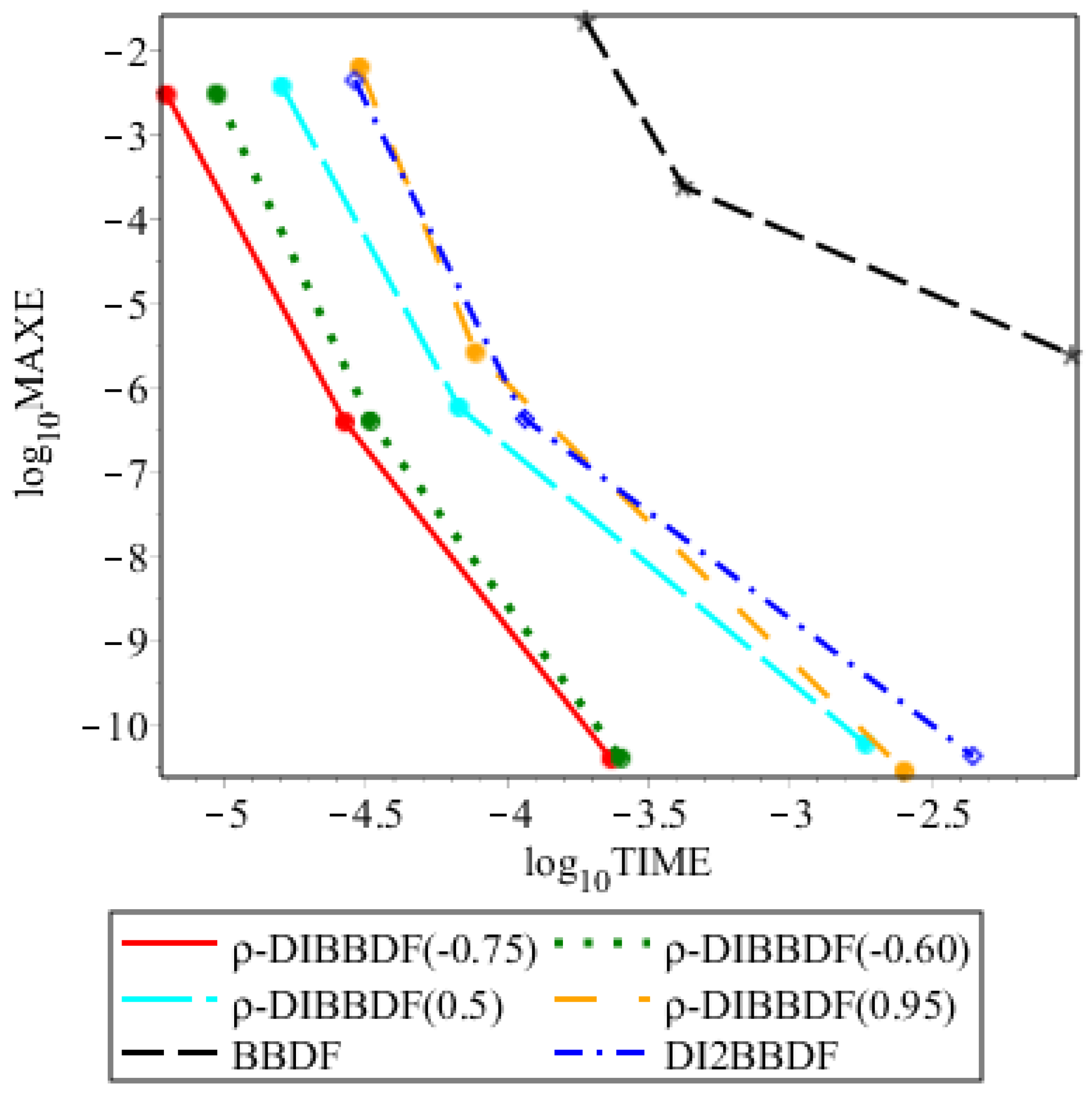
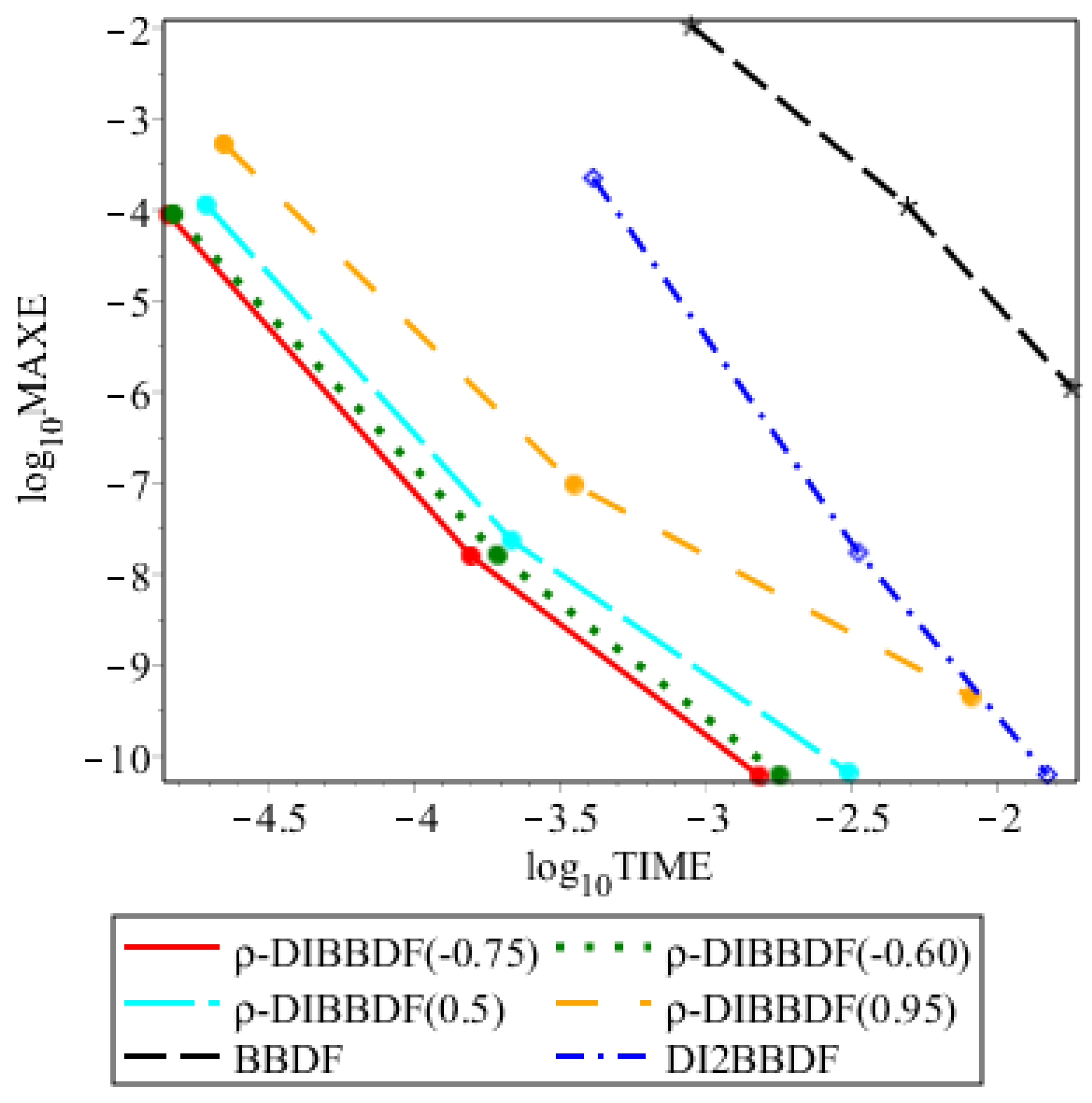
To illustrate the performances of the suggested method and other compared methods, graphical presentations of the numerical results are shown in Figure 4, Figure 5, Figure 6 and Figure 7. For a particular abscissa, the lowest value of the coordinate is considered to be more efficient at the abscissa considered. It follows that the graphs of ${log}_{10}MAXE$ against ${log}_{10}TIME$ demonstrate the advantage of the $\rho$-DIBBDF(−0.75) method over the other $\rho$, BBDF and DI2BBDF methods in terms of efficiency. Overall, we observe that the $\rho$-DIBBDF(−0.75) method performs better than the other $\rho$, BBDF and DI2BBDF methods.

6. Conclusions

In this study, we developed the $\rho$-DIBBDF method with the best choice of the parameter $\rho$ that holds optimal stability properties. The stability analysis shows that this order 3 method is zero stable, $A\left(\alpha \right)$-stable and convergent. Based on Section 3, we noted that the stability properties of the methods compared in Table 2 are related to the MAXE obtained in Section 5. By choosing the best value for the parameter $\rho$, we developed a method that possesses a smaller error constant, a reasonably big $\alpha$ and a larger stability region than the compared methods, thus leading to more accurate results. The proposed method performed better with higher accuracy and less execution time compared to the existing methods, BBDF and DI2BBDF because the DI structure applied to the formula led to an efficient implementation.

Therefore, we conclude that the $\rho$-DIBBDF method has significance as an efficient numerical method for solving stiff first order ODEs.

References

1. Rockswold, G.K. Implementation of α-type multistep methods for stiff differential equations. J. Comput. Appl. Math. 1988, 22, 63–69. [Google Scholar] [CrossRef]
2. Ismail, G.A.F.; Ibrahim, I.H. New efficient second derivative multistep methods for stiff systems. Appl. Math. Model. 1999, 23, 279–288. [Google Scholar] [CrossRef] [Green Version]
3. Butcher, J.C.; Singh, A.D. The choice of parameters in general linear methods for stiff problems. Appl. Numer. Math. 2000, 34, 59–84. [Google Scholar] [CrossRef]
4. Hojjati, G.; Rahimi Ardabili, M.Y.; Hosseini, S.M. New second derivative multistep methods for stiff systems. Appl. Math. Model. 2006, 30, 466–476. [Google Scholar] [CrossRef]
5. Okuonghae, R.I.; Ikhile, M.N.O. A(α)-stable linear multistep methods for stiff IVPs in ODEs. Mathematica 2011, 50, 73–90. [Google Scholar]
6. Okuonghae, R.I.; Ikhile, M.N.O. On the construction of high order A(α)-stable hybrid linear multistep methods for stiff IVPs in ODEs. Numer. Anal. Appl. 2012, 5, 231–241. [Google Scholar] [CrossRef]
7. Lang, J.; Hundsdorfer, W. Extrapolation-based implicit-explicit peer methods with optimised stability regions. J. Comput. Phys. 2017, 337, 203–215. [Google Scholar] [CrossRef]
8. Lambert, J.D. Computational Methods in Ordinary Differential Equations; John Wiley & Sons, Inc.: New York, NY, USA, 1973. [Google Scholar]
9. Ababneh, O.Y.; Ahmad, R.; Ismail, E.S. Design of new diagonally implicit Runge-Kutta methods for stiff problems. Appl. Math. Sci. 2009, 3, 2241–2253. [Google Scholar]
10. Mohd Zawawi, I.S.; Ibrahim, Z.B.; Othman, K.I. Derivation of diagonally implicit block backward differentiation formulas for solving stiff initial value problems. Math. Probl. Eng. 2015, 2015, 13. [Google Scholar] [CrossRef]
11. Isa, S.; Majid, Z.A.; Ismail, F.; Rabiei, F. Diagonally implicit multistep block method of order four for solving fuzzy differential equations using Seikkala derivatives. Symmetry 2018, 10, 42. [Google Scholar] [CrossRef]
12. Ghawadri, N.; Senu, N.; Fawzi, A.F.; Ismail, F.; Ibrahim, Z.B. Diagonally implicit Runge-Kutta type method for directly solving special fourth-order ordinary differential equations with III-posed problem of a beam on elastic foundation. Algorithms 2019, 12, 10. [Google Scholar] [CrossRef]
13. Crockatt, M.M.; Christlieb, A.J.; Garrett, C.K.; Hauck, C.D. Hybrid methods for radiation transport using diagonally implicit Runge-Kutta and space-time discontinuous Galerkin time integration. J. Comput. Phys. 2019, 376, 455–477. [Google Scholar] [CrossRef]
14. Jana Aksah, S.; Ibrahim, Z.B.; Mohd Zawawi, I.S. Stability analysis of singly diagonally implicit block backward differentiation formulas for stiff ordinary differential equations. Mathematics 2019, 7, 211. [Google Scholar] [CrossRef]
15. Pasic, H. An efficient method for solving implicit and explicit stiff differential equations. Int. J. Numer. Meth. Eng. 2000, 48, 55–78. [Google Scholar] [CrossRef]
16. Ritschel, T. Numerical Methods for Solution of Differential Equations. Bachelor’s Thesis, Technical University of Denmark, Lyngby, Denmark, 2013. [Google Scholar]
17. Norsett, S.P. Semi-Explicit Runge-Kutta Methods; Report Mathematics and Computation No. 6/74; Dept. of Mathematics, Universiti of Trondheim: Trondheim, Norway, 1974. [Google Scholar]
18. Alexander, R. Diagonally implicit Runge-Kutta methods for solving stiff O.D.E.’s. SIAM J. Numer. Anal. 1977, 14, 1006–1021. [Google Scholar] [CrossRef]
19. Skvortsov, L.M. Diagonally implicit Runge-Kutta methods for stiff problems. Comput. Math. Math. Phys. 2006, 46, 2110–2123. [Google Scholar] [CrossRef]
20. Ibrahim, Z.B.; Othman, K.I.; Suleiman, M.B. Implicit r-point block backward differentiation formula for solving first-order stiff ODEs. Appl. Math. Comput. 2007, 186, 558–565. [Google Scholar] [CrossRef]
21. Ibrahim, Z.B.; Suleiman, M.B.; Othman, K.I. Fixed coefficients block backward differentiation formulas for the numerical solution of stiff ordinary differential equations. Eur. J. Sci. Res. 2008, 21, 508–520. [Google Scholar]
22. Suleiman, M.B.; Musa, H.; Ismail, F.; Senu, N.; Ibrahim, Z.B. A new superclass of block backward differentiation formula for stiff ordinary differential equations. Asian-Eur. J. Math. 2014, 7, 1–17. [Google Scholar] [CrossRef]
23. Mohd Nasir, N.A.A.; Ibrahim, Z.B.; Suleiman, M.B.; Othman, K.I.; Rahim, Y.F. Numerical solution of tumor-immune interaction using 2-point block backward differentiation method. Int. J. Mod. Phys. Conf. Ser. 2012, 9, 278–284. [Google Scholar] [CrossRef]
24. Mohd Yatim, S.A.; Ibrahim, Z.B.; Othman, K.I.; Suleiman, M.B. A numerical algorithm for solving stiff ordinary differential equations. Math. Probl. Eng. 2013, 2013, 11. [Google Scholar]
25. Gear, C.W. Algorithm 407: DIFSUB for solution of ordinary differential equations. Commun. ACM 1971, 14, 185–190. [Google Scholar] [CrossRef]
26. Vijitha-Kumara, K.H.Y. Variable Stepsize Variable Order Multistep Methods for Stiff Ordinary Differential Equations. Ph.D. Thesis, Iowa State University, Ames, IA, USA, 1985. [Google Scholar]
27. Dahlquist, G. A special stability problem for linear multistep methods. BIT 1963, 3, 27–43. [Google Scholar] [CrossRef]
28. Ibrahim, Z.B.; Mohd Noor, N.; Othman, K.I. Fixed coefficient A(α) stable block backward differentiation formulas for stiff ordinary differential equations. Symmetry 2019, 11, 846. [Google Scholar] [CrossRef]
29. Liniger, W. A criterion for A-stability of linear multistep integration formulae. Computing 1968, 3, 280–285. [Google Scholar] [CrossRef]
30. Rockswold, G.K. Stable Variable Step Stiff Methods for Ordinary Differential Equations. Ph.D. Thesis, Iowa State University, Ames, IA, USA, 1983. [Google Scholar]
31. Jeltsch, R. Stiff stability and its relation to A0- and A(0)-stability. SIAM J. Numer. Anal. 1976, 13, 8–17. [Google Scholar] [CrossRef]
32. Lambert, J.D. Numerical Methods for Ordinary Differential Systems: The Initial Value Problem; John Wiley & Sons, Inc.: New York, NY, USA, 1991. [Google Scholar]
33. Widlund, O.B. A note on unconditionally stable linear multistep methods. BIT 1967, 7, 65–70. [Google Scholar] [CrossRef]
34. Butcher, J.C. Forty-five years of A-stability. J. Numer. Anal. Ind. Appl. Math. 2009, 4, 1–9. [Google Scholar]
35. Hall, G.; Watt, J.M. Modern Numerical Methods for Ordinary Differential Equations; Clarendon Press: Oxford, UK, 1976. [Google Scholar]
36. Kushnir, D.; Rokhlin, V. A highly accurate solver for stiff ordinary differential equations. SIAM J. Sci. Comput. 2011, 34, 1296–1315. [Google Scholar] [CrossRef]
37. Lee, H.C.; Chen, C.K.; Hung, C.I. A modified group-preserving scheme for solving the initial value problems of stiff ordinary differential equations. Appl. Math. Comput. 2002, 133, 445–459. [Google Scholar] [CrossRef]
Figure 1. Structure of the A-matrix for fully and diagonally implicit subclasses of the RK methods, given in [16].
Symmetry 11 01342 g001
Figure 2. A ( α ) and stiff stability, as featured in [34].
Symmetry 11 01342 g002
Figure 3. Stability region of ρ -DIBBDF for ρ = - 0 . 75 .
Symmetry 11 01342 g003
Figure 4. Efficiency curves for test problem 1.
Symmetry 11 01342 g004
Figure 5. Efficiency curves for test problem 2.
Symmetry 11 01342 g005
Figure 6. Efficiency curves for test problem 3.
Symmetry 11 01342 g006
Figure 7. Efficiency curves for test problem 4.
Symmetry 11 01342 g007