Type 2 Fuzzy Inference-Based Time Series Model


1
Centre for Pre University Studies, Universiti Malaysia Sarawak, Kota Samarahan, Sarawak 94300, Malaysia
2
Fundamental and Applied Sciences Department, Universiti Teknologi PETRONAS, Seri Iskandar, Perak 32610, Malaysia
3
Faculty of Engineering, Universitas Islam Riau, Pekan Baru, Riau 28284, Indonesia
*
Author to whom correspondence should be addressed.
Symmetry 2019, 11(11), 1340; https://doi.org/10.3390/sym11111340
Submission received: 25 September 2019
/
Revised: 18 October 2019
/
Accepted: 22 October 2019
/
Published: 31 October 2019
(This article belongs to the Special Issue Fuzzy Mathematics Applied to Science, Engineering and Sustainability Issues)
Abstract
:Fuzzy techniques have been suggested as useful method for forecasting performance. However, its dependency on experts’ knowledge causes difficulties in information extraction and data collection. Therefore, to overcome the difficulties, this research proposed a new type 2 fuzzy time series (T2FTS) forecasting model. The T2FTS model was used to exploit more information in time series forecasting. The concepts of sliding window method (SWM) and fuzzy rule-based systems (FRBS) were incorporated in the utilization of T2FTS to obtain forecasting values. A sliding window method was proposed to find a proper and systematic measurement for predicting the number of class intervals. Furthermore, the weighted subsethood-based algorithm was applied in developing fuzzy IF–THEN rules, where it was later used to perform forecasting. This approach provides inferences based on how people think and make judgments. In this research, the data sets from previous studies of crude palm oil prices were used to further analyze and validate the proposed model. With suitable class intervals and fuzzy rules generated, the forecasting values obtained were more precise and closer to the actual values. The findings of this paper proved that the proposed forecasting method could be used as an alternative for improved forecasting of sustainable crude palm oil prices.
1. Introduction
There are a number of ways to obtain forecast value in the analysis of time series [1] such as artificial intelligence approaches [2], artificial neural network (ANN) [3,4] and autoregressive integrated moving average (ARIMA) models [1,5]. According to [6], the selection of the methods must reflect several features such as data and degree of significance. Nevertheless, most of the previous models are quite costly and require expertise and several data types that are occasionally unobtainable.
The fuzzy time series (FTS) method was widely used in different applications to solve forecasting problems. It was discussed in many types of research [7,8,9] such as in weather forecasting, stock fluctuations, and any situation in which variables change unpredictability over time. As the issues on forecasting with data on past events are linguistic values, the common method of time series forecasting methods is not relevant to be used [10]. FTS has been improved by many researchers to produce the most ideal forecasting outcomes [11]. The studies in [12,13,14] suggested time-variant and time-invariant FTS models in forecasting and their observations are in terms of linguistics values. In addition, the research in [15,16] used a simple arithmetic operation instead of complicated maximum and minimum composition operations in time series forecasting. Thereafter, many previous research works were revealed to reduce forecasting error and computational overload.
In developing a FTS model, the universe of discourse must be divided into a certain length of interval. This is because the interval length factor can affect the FTS model performance. Sliding window method (SWM) is an interesting topic to be considered in solving this interval length issue. The SWM was introduced by [17], in which it is used for time series analysis, and it is appropriate for many applications [18]. The applications of SWM can be found in various disciplines, for example, medicine [19], weather forecasting [18,20], and database system [21]. In previous studies, limited class interval was used for FTS forecasting. It was mentioned in [22] that the interval length is essential in forecasting performance. Hence, techniques to find intervals using mean and data distributions were proposed. A few years later, [23] suggested the division of the interval by using ratios rather than equal lengths of intervals, where it was believed that it can represent the intervals of the observations properly. Thus, by introducing SWM in time series forecasting, there is a specific method in handling and determining the class interval with suitable interval length.
Researchers in [24] mentioned that fuzzy rules are also important elements that are highlighted in any fuzzy expert system. It is widely used to carry out numerous real-world classification tasks. However, to obtain high classification accuracy, the transparency and interpretability of such models are often ignored. Forecasting consists of a few elements that involve imprecise data and are always based on the number of judgments. This fuzziness is from human clarification of future data values [25]. A reasoning-based model is expected to offer an alternative approach to handling many kinds of inaccurate data that reflect human thinking and decision making. It is able to make an inference of various attributes that contain imprecise data [26,27,28]. Specifically, intuitive methods of analysis that are done according to linguistic models, fuzzy rule-based systems (FRBS), have successfully solved real-world issues.
Current evolution in reasoning based on linguistic models provide evidence of the significant role of FRBS in allowing a worthy explanation of inference in terms of linguistic statements with a higher percentage of accuracy. These linguistic rule models illustrate the actual way humans consider issues and form judgments. One of the typical examples of the linguistic rule can be found in [27]. Easiness in creating fuzzy rules with the capability of increasing the classification precision level is the intention of proposing the weighted subsethood-based algorithm (WSBA). Therefore, the fuzzy subsethood measures and weighted linguistic fuzzy models are the elements that can provide advantages to the FTS.
Nevertheless, most conventional FTS models such as type 1 fuzzy time series forecasting models utilize a single forecasting variable and certain observations related to the variable [29]. The change of variable value for some complex models is not only caused by its rules but can also be influenced by other factors. Furthermore, it is difficult to handle forecasting problems using conventional FTS if the past events data are in terms of linguistic values [30]. Hence, a new method, type 2 fuzzy time series (T2FTS) model, was suggested to get the benefit of the related element and solve the forecasting problem indirectly.
The identified problems of this research can be recapitulated as follows. Although there are several methods of time series forecasting, there continue to be arguments that the inputs required to sustain the manufacture of numerous products are to be decided by the forecaster. In addition, the volatility due to uncertainties is the main concern. As can be seen in various cases, there are limitations in terms of accuracy of the forecasting values. Finding a suitable method in forecasting application is the difficulty that a forecaster faces. Therefore, the use of a fuzzy method is beneficial in controlling the vagueness within the data and minimizing the error of forecasting. Even though previous methods are suitable in determining the forecasting precision, the methods do not look into the application of fuzzy approximate reasoning which indicates individual’s opinion.
Another concern in many forecasting methods is the extent to which the method is able to lessen the error of forecasting. The previous methods are also unable to generate precise forecast values. Furthermore, the fuzzy rule system consists of rules constructed from input data. The efficiency or accuracy of the fuzzy system is proportional to the accurateness of the rule defined. The appropriateness of the rule constructed is where it could summarize the data in grasping the meaning of a large collection of data. Thus, there is a need to discover a better approach for forecasting that can solve these issues. In thisresearch, type 2 fuzzy time series (T2FTS) forecasting that is systematic and flexible, together with a reasoning-based model, which is the sliding window method and weighted subsethood-based algorithm, was applied to address this uncertainty. Moreover, to improve the forecasting value, this research extended the observation using T2FTS. By utilizing extra observations in the proposed forecasting method, it was hypothesized that the forecasting results would be improved.
Generally, this research proposed a new T2FTS model to forecast accurate future data values with minimum forecasting error. Specifically, this research suggests a new approach of sliding window method in determining the number of the class intervals of the universe of discourse of FTS. Secondly, this research develops a fuzzy rule-based system using weighted subsethood-based algorithm (WSBA) in FTS forecasting. Third, this paper exploited more variables of observations in forecasting using a new T2FTS model. All the three objectives were utilized to refine the optimum numbers of intervals and created fuzzy ruled based relationships. Thereby, forecasting performance could be improved. The detailed explanation is given in Section 2.
This research was compared to Chen’s model since the rule used by Chen’s model was based on expert opinion, while this research used weighted subsethood-based algorithm to generate new fuzzy rules. Furthermore, Chen’s model only used a single variable of observation. Whereas, this research utilized more variable of observations and used type 2 fuzzy time series to forecast the crude palm oil (CPO) prices.
The subsequent sections highlight the methodology of this paper, followed by illustration of the empirical analysis of the proposed forecasting method on the price of crude palm oil (CPO). The next section lists the algorithm of the proposed method. The following section elaborates the analysis outcomes and discussion on the forecasted CPO prices obtained. Finally, the last section of this paper is the summary of this research.
2. Methodology
The methodology section highlights the flow of the method implemented in meeting the aim of this research. This research involved three stages. This section also explains the mathematical formulae and techniques that were used to obtain the results. Further explanation is as follows.
2.1. Collection and Selection of Data
This research uses data sets from previous researches. For validation purposes, this research uses the daily price of crude palm oil (CPO) data in Malaysia, from the year 2012 to 2016. The data were taken from the Malaysian Palm Oil Board (MPOB). These empirical data were used in the research analysis to forecast the distribution of the existing data. The data were divided into two sets; one data set was used for estimation and the other data set was used for forecasting purposes [25]. To perform the estimation, the data were taken between January and October every year, while the November and December data were utilized for forecasting.
2.2. Proposed Forecasting Model
In this phase, there were several steps of the type 2 fuzzy time series (T2FTS) model that were implemented. The further illustrations are as follows.
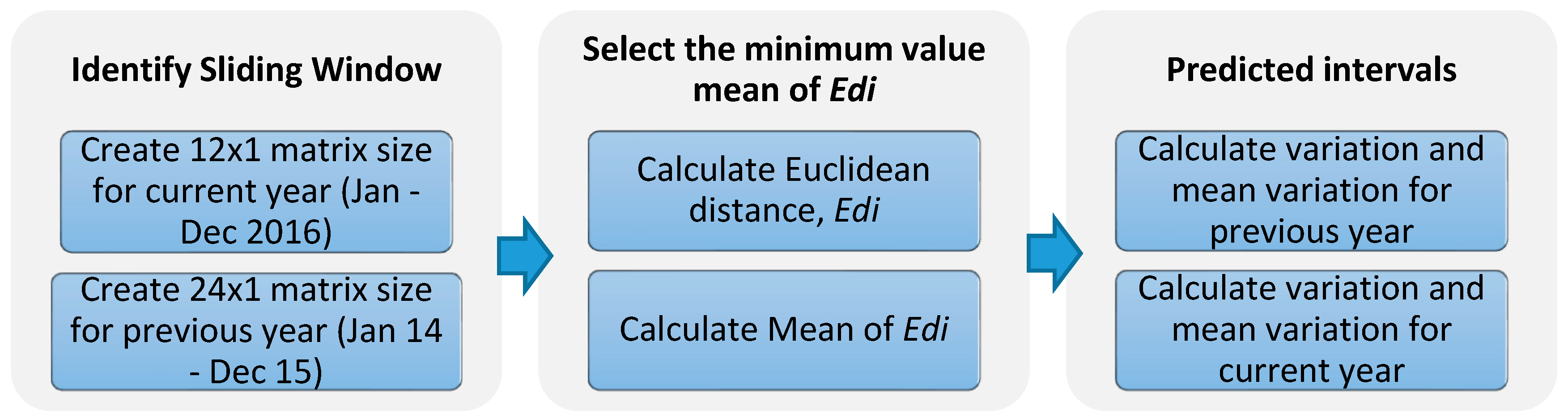
To develop a fuzzy time series (FTS) model, the universe of discourse, U, needs to be defined and partitioned into a certain length by determining the class intervals. Among FTS models, the model in [15] offers the easiest calculations and delivers good forecasting results. Hence, this research followed an interval FTS model for the purpose of illustration. In this step, the sliding window method was implemented in order to determine the class intervals. Figure 1 shows the sliding window algorithm.
This research continues with fuzzifying the observations into corresponding fuzzy sets. By using the intervals obtained, the fuzzy sets were defined for observations. Then, the fuzzy logical relationship group (FLRG) is acquired, as specified in Equation (1),
where indicates the fuzzy relationship towards previous data, and current data, , and * denotes the operator. These relationships are attributed as a fuzzy logical relationship (FLR) [31,32], where and . It is expressed as , where is termed as the left hand side (LHS) and the right hand side (RHS) of the FLR.
In these models, the FLRs are mixed into fuzzy logical relationship groups (FLRGs). Similar LHSs of the FLRs were put together and the LHSs continued as the LHS while the RHSs combined as the RHS. Equation (2) depicts the FLRs that have been gathered into a FLRG.
Then, the highest and lowest values were chosen as Type 2 observations and the out-of-sample observation was mapped into FLRGs, including Type 1 and 2 observations. In this research, the lowest and highest crude palm oil (CPO) prices were selected.
To obtain forecasts, operators and the fuzzy rules obtained were applied to the FLRGs for each of the observations. The weighted subsethood-based algorithm which referred to [33] was used to develop the fuzzy rules. These operators and fuzzy rules were used to screen out or include the fuzzy relationships of the observations. The forecasts were obtained from these fuzzy relationships.
In this research, two operators were used, which are screening out () and including () fuzzy relationship. These union and intersection operators were proposed in the Type 2 model correspondingly, as in [29].
Equations (3) and (4) define the Union () and intersection () operators, which were used to establish the relationships between the two fuzzy logical relationship groups (FLRGs):
where refers to the union and is the intersection operator for the set theory, while left-hand side, and right-hand side, were the LHS and RHS of an FLRG, d, respectively.
Then, defuzzification was performed and the forecast values were calculated using Equations (5) and (6), respectively [29].
where is a defuzzified forecast done according to a Type 2 observation, with a total of e Type 2 observations at time t. Supposing the forecast is fuzzy sets, Aq1; Aq2; ... ; Aqj; the defuzzified forecast is equal to the arithmetic average of mq1; mq2; ... ; mqj; the midpoints of intervals, uq1; uq2; ... ; uqj; respectively [11].
2.3. Evaluation of the Performance
Once the forecasts value was obtained, the root mean square error (RMSE) was used for the evaluation of the forecasting performance, where actualt is the actual price, defuzzification(t) is the defuzzified forecast and there were n forecasts as shown in Equation (7).
3. Empirical Analysis
The forecasting for each data was conducted as follows. For illustration purposes, this research discusses the analysis using the price data of crude palm oil (CPO) for the year 2012.
First, the highest and lowest CPO prices in the year 2012 were determined: , . Hence, the universe of discourse was divided into certain lengths of interval, where the intervals were determined using a sliding window method which was adopted from [20].
In 2012, there were 47 intervals with the same lengths of 5: , ,…, where the intervals’ midpoints are …, From the intervals obtained, the fuzzy sets, for observations were defined. Every was described by the intervals, .
This research continued with fuzzifying the observations. Table 1 listed some of the fuzzified CPO prices for the year 2012. The data from January to October were used to perform estimation. While the data for November and December were utilized for forecasting.
Figure 2 depicts some of the fuzzification process for the year 2012.
Next, the fuzzy relationships were obtained. The FLRs can be established by combining two consecutive fuzzy sets. Referring to Table 1, the CPO prices for 2012/10/7 is and for 2012/10/8 it is . Hence, it could be established that the FLR is . Therefore, the FLRs etc. can be established. Table 2 lists an example of the FLRs for the year 2012 and some were obtained from Table 1.
Based on Table 2, the FLRs with the same LHSs can be located together. For example,
A FLRG with can be grouped as the LHS such that
Table 3 shows the fuzzy logical relationship groups (FLRGs).
Then, the highest and lowest daily prices for CPO price were picked as Type 2 observations. Table 4 depicts some of the information in 2012 for further clarification.
According to Table 4, on 10/11, the fuzzy set for the closing is , the high is , and the low is , respectively. On 10/12, the fuzzy set for closing is , the high is , and the low is . Meanwhile, on 10/13, the fuzzy set for closing is , the high is , and the low is .
Next, observations made on the out-of-sample were mapped out, which included the Type 1 and Type 2 observations, to the FLRGs to obtain forecast values. For instance, given that is , and the forecast for is . Table 5 and Table 6 are the forecasts obtained for the observations.
The research applies operators and fuzzy rules that were generated using the weighted subsethood-based algorithm for each date of the forecasts as in [33]. In Table 5, the research applies (intersection operator) to all the forecasts obtained. Similarly, Table 6 lists the forecasts, in which it applied (union operator) to all the forecasts.
Then, the forecasts were defuzzified using Equation (5). Refer to Table 5, for , the forecast for the date 10/12 is . is the defuzzified forecast of , which is 421.50. In other words, . Again, the forecast for the date 10/13 is . Hence, . The forecast for the date 10/14 is ; .
For , the forecast for 10/12 is , as well as . The defuzzified forecast is as follows.
The forecast for the date 10/13 is and . The value of the defuzzified forecast is
The forecast for the date 10/14 is and . The defuzzified forecast obtained is
Then, the forecasting values for Type 2 model were computed using Equation (6).
Therefore,
Similarly,
Therefore,
Hence,
Last but not least, this research evaluated the forecasting performance using RMSE as in Equation (7).
4. Algorithm of the Proposed Method
The outline of the abovementioned analysis is summarizing into the algorithm of type 2 fuzzy time series (T2FTS) model, as follows.
- Step 1:
- The class interval of the universe of discourse is determined by using the sliding window method.
- Step 2:
- The observations are fuzzified into corresponding fuzzy sets.
- Step 3:
- Fuzzy logical relationship groups (FLRGs) are obtained.
- Step 4:
- Out-of-sample observations are mapped to FLRGs.
- Step 5:
- Operators and fuzzy rules obtained by using weighted subsethood-based algorithm are applied to the FLRGs for all the observations and obtain forecasts.
- Step 6:
- The forecasts are defuzzified.
- Step 7:
- Forecast values are computed for all data individually.
- Step 8:
- The method is compared with the previous method.
5. Results and Discussion
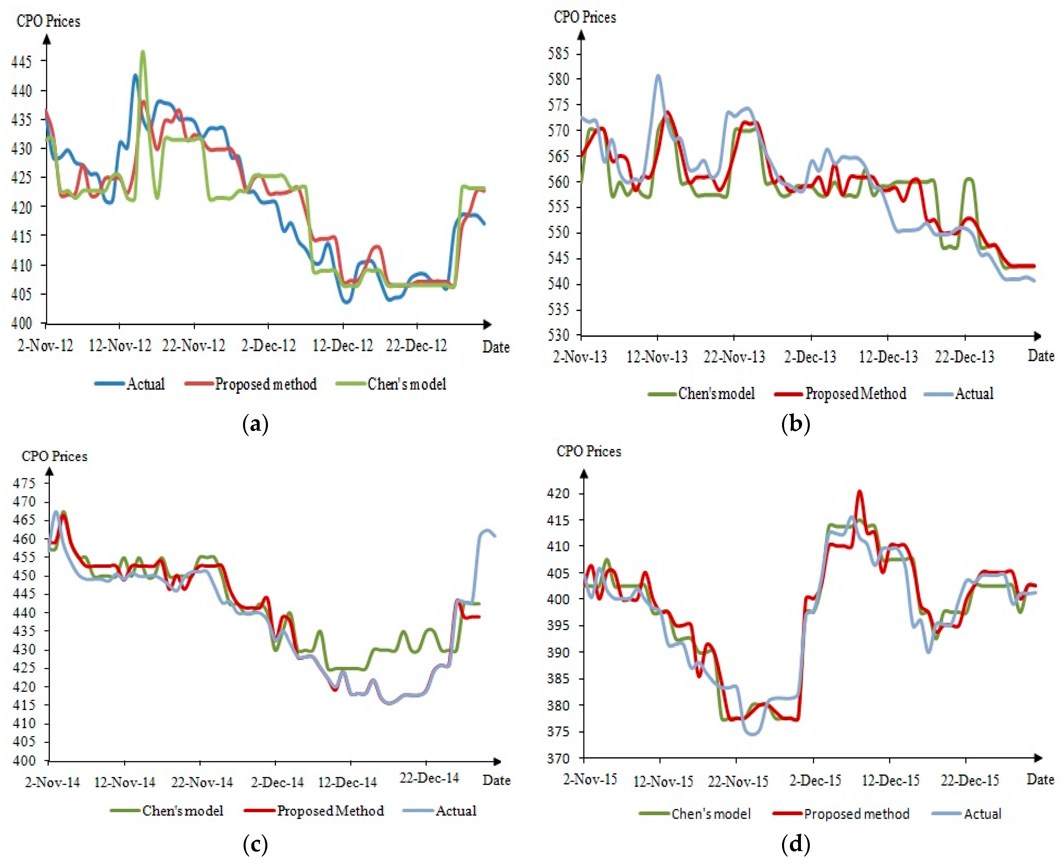
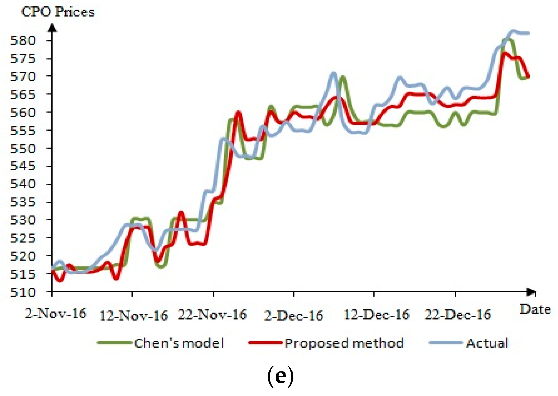
The analysis of the forecasted price of CPO generated is discussed in this section. The out-of-sample defuzzified forecast for this method and Chen’s model [15] for each year (November to December) are depicted in Figure 3a–e.
In Figure 3, the blue line is the real CPO price, the red line is the forecast value using the proposed method, while the green line is the forecast value using Chen’s model. From the graphs, the forecast value of CPO prices obtained from the proposed method is deemed better compared to the forecast value obtained using Chen’s model. In support of this statement, the percent error for each year was determined, as shown in Table 7, which was calculated using Equation (7).
From the result in Table 7, Chen’s model has a higher rate of error compared to the proposed method. This indicates that this method is capable of reducing forecasting errors from Chen’s model and forecasting consistently.
6. Conclusions
Most conventional fuzzy time series (FTS) forecasting models use one variable in forecasting and not all the observations are related to the variable. In real forecasting situations where more complex models are involved, the change of dependent variable value is influenced by other determinants. Therefore, the use of conventional fuzzy time series is difficult when solving real forecasting problems [30]. Hence, this research proposes a new approach of type 2 fuzzy time series (T2FTS) models to exploit an extra observation. To increase the level of efficiency of this method, the sliding window method and the weighted subsethood-based algorithm were implemented in this model. The forecast values obtained from the use of the proposed method were then compared to Chen’s model. The forecast error was tested through the use of root mean squared error (RMSE) for both methods. The outcome of the RMSEs using the proposed method is less than that for Chen’s model. This demonstrates that the proposed method is capable of giving a superior forecast compared to Chen’s model. Hence, the employment of the proposed method will lead to the creation of an efficient approach in forecasting application which will support decisions made by alternative methods indirectly. This research proposes an extension of the current research in achieving a universal view of suitable combination of factors as well as the classification of the class interval. Thus, this method could enhance the capability of the proposed type 2 fuzzy time series (T2FTS) models. The use of crude palm oil is dependent upon its price. Therefore, the price of crude palm oil determines its usage for plantation activities. For instance, the price of crude palm oil influences its use in mills as well as feedstock for biodiesel. The price of crude palm oil also determines other plantation activities including the preparation of plantation land. Failure to forecast crude palm oil prices may cause plantations to use fire as a low-cost solution. The resulting environmental impacts include deforestation, biodiversity loss, water and air pollution, such as haze, and emission of greenhouse gases. The price of crude palm oil has social impacts such as land use rights; smallholders including livelihoods, income, and wellbeing; forced and child labor, and terms and conditions of labor including wages and health and safety. Thus, this research offers a sustainable palm oil price forecasting model which helps the government and palm oil industries in making business decisions and to understand strategies of major players in the industry.
Author Contributions
Project administration, N.F.R.; supervision, M.O., R.S. and E.A.K.
Funding
This research was funded by the Grant Fundamental Research Grant Scheme (FRGS), Universiti Teknologi PETRONAS, cost center: 015MA0-021.
Acknowledgments
Many thanks to Universiti Teknologi PETRONAS for providing financial support and good facilities.
Conflicts of Interest
The authors declare no conflict of interest.
References
- Ahmad, M.H.; Ping, P.Y.; Mahamed, N. Volatility modelling and forecasting of Malaysian crude palm oil prices. Appl. Math. Sci. 2014, 8, 6159–6169. [Google Scholar] [CrossRef] [Green Version]
- Karia, A.A.; Bujang, I.; Ahmad, I. Forecasting on crude palm oil prices using artificial intelligence approaches. Am. J. Oper. Res. 2013, 3, 259–267. [Google Scholar] [CrossRef]
- Luk, K.C.; Ball, J.E.; Sharma, A. An application of artificial neural networks for rainfall forecasting. Math. Comput. Model. 2001, 33, 683–693. [Google Scholar] [CrossRef]
- Hung, N.Q.; Babel, M.S.; Weesakul, S.; Tripathi, N.K. An artificial neural network model for rainfall forecasting in Bangkok, Thailand. Hydrol. Earth Syst. Sci. 2008, 13, 1413–1425. [Google Scholar] [CrossRef]
- Fatimah, M.A.; Hameed, A. Crude oil, palm oil stock and prices: How they link. Rev. Econ. Financ. 2013, 3, 48–57. [Google Scholar]
- Applanaidu, S.D.; Fatimah, M.A.; Shamsudin, M.N.; Abdel Hameed, A.A. An econometric analysis of the link between biodiesel demand and malaysian palm oil market. Int. J. Bus. Manag. 2011, 6, 35–45. [Google Scholar] [CrossRef]
- Tanuwijaya, K.; Chen, S.M. A new method to forecast enrollments using fuzzy time series and clustering techniques. In Proceedings of the 2009 international conference on machine learning and cybernetics, Hebei, China, 12–15 July 2009. [Google Scholar]
- Wang, Y.N.; Lei, Y.; Fan, X.; Wang, Y. Intuitionistic fuzzy time series forecasting model based on intuitionistic fuzzy reasoning. Math. Probl. Eng. 2016, 38, 1332–1338. [Google Scholar] [CrossRef]
- Uslu, V.R.; Bas, E.; Yolcu, U.; Egrioglu, E. A new fuzzy time series analysis approach by using differential evolution algorithm and chronologically-determined weights. J. Soc. Econ. Stat. 2013, 2, 18–30. [Google Scholar]
- Rajaram, S.; Vamitha, V. A modified approach on fuzzy time series forecasting. Ann. Pure Appl. Math. 2012, 2, 96–106. [Google Scholar]
- Chen, S.M.; Hsu, C.C. A new method to forecast enrollments using fuzzy time series. Int. J. Appl. Sci.& Eng. 2004, 2, 234–244. [Google Scholar]
- Song, Q.; Chissom, B.S. Fuzzy time series and its models. Fuzzy Sets Syst. 1993, 54, 269–277. [Google Scholar] [CrossRef]
- Song, Q.; Chissom, B.S. Forecasting enrollments with fuzzy time series—Part I. Fuzzy Sets Syst. 1993, 54, 1–9. [Google Scholar] [CrossRef]
- Song, Q.; Chissom, B.S. Forecasting enrollments with fuzzy time series—Part II. Fuzzy Sets Syst. 1994, 62, 1–8. [Google Scholar] [CrossRef]
- Chen, S. Forecasting enrollments based on fuzzy time series. Fuzzy Sets Syst. 1996, 81, 311–319. [Google Scholar] [CrossRef]
- Saxena, P. Forecasting enrollments based on fuzzy time series with Higher Forecast Accuracy Rate. Int. J. Comput. Technol. Appl. 2012, 3, 957–961. [Google Scholar]
- Datar, M.; Gionis, A.; Indyk, P.; Motwani, R. Maintaining stream statistics over sliding windows: (extended abstract). In Proceedings of the Thirteenth Annual {ACM-SIAM} Symposium on Discrete Algorithms, San Francisco, CA, USA, 6–8 January 2002; pp. 635–644. [Google Scholar]
- BenYahmed, Y.; Abu, B.A.; Razak, H.A.; Ahmed, A.; Abdullah, S.M.S. Adaptive sliding window algorithm for weather data segmentation. J. Theor. Appl. Inf. Technol. 2015, 80, 322–333. [Google Scholar]
- D’Arcy, J.A.; Collins, D.J.; Rowland, I.J.; Padhani, A.R.; Leach, M.O. Applications of sliding window reconstruction with cartesian sampling for dynamic contrast enhanced MRI. NMR Biomed. 2002, 15, 174–183. [Google Scholar] [CrossRef]
- Kapoor, P.; Bedi, S.S. Weather forecasting using sliding window algorithm. ISRN Signal. Process. 2013, 2013, 1–5. [Google Scholar] [CrossRef]
- Arasu, A.; Manku, G.S. Approximate counts and quantiles over sliding windows. In Proceedings of the twenty-third ACM SIGMOD-SIGACT-SIGART symposium on Principles of database systems, Paris, France, 14–16 June 2004; pp. 286–296. [Google Scholar]
- Huarng, K. Effective lengths of intervals to improve forecasting in fuzzy time series. Fuzzy Sets Syst. 2001, 123, 387–394. [Google Scholar] [CrossRef]
- Huarng, K.; Yu, T.H. Ratio-based lengths of intervals to improve fuzzy time series forecasting. IEEE Trans. Syst. Man. Cybern. B Cybern. 2006, 36, 328–340. [Google Scholar] [CrossRef]
- Rasmani, K.A.; Shen, Q. Subsethood-based fuzzy modelling and classification. In Proceedings of the 14th IEEE International Conference On Fuzzy Systems, Reno, NV, USA, 25 May 2005. [Google Scholar]
- Rasmani, K.A.; Shen, Q. Data-driven fuzzy rule generation and its application for student academic performance evaluation. Appl. Intell. 2006, 25, 305–319. [Google Scholar] [CrossRef] [Green Version]
- Cordón, O.; Herrera, F.; Zwir, I. Linguistic modeling by hierarchical systems of linguistic rules. IEEE Trans. Fuzzy Syst. 2002, 10, 2–20. [Google Scholar] [CrossRef]
- Dubois, D.; Prade, H. Handbook of fuzzy computation. Fuzzy Sets Syst. Dep. Comput. Sci. Artif. Intell. 2001, 123, 397–398. [Google Scholar] [CrossRef]
- Khaliq, A.; Ahmad, A. Fuzzy Logic and Approximate Reasoning; Blekinge Institute of Technology: Karlskrona, Sweeden, 2010. [Google Scholar]
- Huarng, K.; Yu, H.K. A Type 2 fuzzy time series model for stock index forecasting. Phys. Stat. Mech. Appl. 2005, 353, 445–462. [Google Scholar] [CrossRef]
- Zhang, E.; Wang, D.; Li, H. A comprehensive high order Type 2 fuzzy time series forecasting model. In Proceedings of the 28th Chinese control and decision conference, Shenyang, China, 28–30 May 2016; pp. 6681–6686. [Google Scholar]
- Maleki, A.; Pasha, E.; Razzaghnia, T. Possibility linear regression analysis with trapezoidal fuzzy data. World Appl. Sci. J. 2012, 18, 37–42. [Google Scholar]
- Chen, S.M.; Wang, N.Y. Fuzzy forecasting based on fuzzy-trend logical relationship groups. IEEE Trans. Syst. Man. Cybern. Part. B Cybern. 2010, 40, 1343–1358. [Google Scholar] [CrossRef]
- Rahim, N.F.; Othman, M.; Sokkalingam, R.; Abdul, K.E. Forecasting crude palm oil prices using fuzzy rule-based time series method. IEEE Access 2018, 6, 32216–32224. [Google Scholar] [CrossRef]
Figure 1.
Sliding window algorithm.

Figure 2.
Fuzzified process.

Figure 3.
Performance comparison: (a) Year 2012; (b) Year 2013; (c) Year 2014; (d) Year 2015; (e) Year 2016.
Figure 3.
Performance comparison: (a) Year 2012; (b) Year 2013; (c) Year 2014; (d) Year 2015; (e) Year 2016.

Table 1.
Fuzzy crude palm oil (CPO) prices (October 2012).
| Date (yyyy/mm/dd) | CPO Price | Fuzzy Sets |
|---|---|---|
| 2012/10/1 | 424.20 | A7 |
| 2012/10/2 | 424.20 | A7 |
| 2012/10/3 | 407.40 | A3 |
| 2012/10/4 | 395.20 | A1 |
| 2012/10/5 | 411.00 | A4 |
| 2012/10/6 | 412.50 | A4 |
| 2012/10/7 | 412.50 | A4 |
| 2012/10/8 | 406.80 | A3 |
| 2012/10/9 | 418.50 | A5 |
| 2012/10/10 | 418.00 | A5 |
| 2012/10/11 | 430.00 | A8 |
| 2012/10/12 | 423.00 | A6 |
| 2012/10/13 | 415.50 | A5 |
| 2012/10/14 | 415.50 | A5 |
| 2012/10/15 | 417.40 | A5 |
| 2012/10/16 | 417.00 | A5 |
| 2012/10/17 | 414.90 | A5 |
| 2012/10/18 | 419.60 | A6 |
| 2012/10/19 | 425.80 | A7 |
| 2012/10/20 | 424.00 | A6 |
| 2012/10/21 | 424.00 | A6 |
| 2012/10/22 | 435.10 | A9 |
| 2012/10/23 | 424.70 | A7 |
| 2012/10/24 | 424.70 | A7 |
| 2012/10/25 | 435.20 | A9 |
| 2012/10/26 | 435.20 | A9 |
| 2012/10/27 | 434.30 | A9 |
| 2012/10/28 | 434.30 | A9 |
| 2012/10/29 | 428.60 | A7 |
| 2012/10/30 | 426.00 | A7 |
| 2012/10/31 | 424.70 | A7 |
Table 2.
Fuzzy logic relationships.
Table 3.
Fuzzy logical relationship groups.
Table 4.
Data for forecasting.
| Date (mm/dd) | Closing | High | Low |
|---|---|---|---|
| … | … | … | … |
| 10/11 | 430.00 | 431.10 | 419.20 |
| 10/12 | 423.00 | 428.80 | 412.80 |
| 10/13 | 415.50 | 420.30 | 413.80 |
| … | … | … | … |
Table 5.
Forecasts after .
| Date (mm/dd) | Forecasts | ||
|---|---|---|---|
| Closing | |||
| 10/12 | High | ||
| Low | |||
| Closing | |||
| 10/13 | High | ||
| Low | |||
| Closing | |||
| 10/14 | High | ||
| Low |
Table 6.
Forecasts after .
| Date (mm/dd) | Forecasts | ||
|---|---|---|---|
| Closing | |||
| 10/12 | High | ||
| Low | |||
| Closing | |||
| 10/13 | High | ||
| Low | |||
| Closing | |||
| 10/14 | High | ||
| Low |
Table 7.
Model evaluation.
| Year | Mean Square Error (MSE) | Root Mean Square Error (RMSE) | ||
|---|---|---|---|---|
| Proposed Method | Chen’s model | Proposed Method | Chen’s model | |
| 2012 | 0.0010 | 0.0010 | 0.518 | 0.520 |
| 2013 | 0.00067 | 0.0011 | 0.457 | 0.635 |
| 2014 | 0.0019 | 0.0027 | 0.637 | 0.855 |
| 2015 | 0.00069 | 0.00079 | 0.414 | 0.462 |
| 2016 | 0.0009 | 0.0015 | 0.567 | 0.754 |
© 2019 by the authors. Licensee MDPI, Basel, Switzerland. This article is an open access article distributed under the terms and conditions of the Creative Commons Attribution (CC BY) license (http://creativecommons.org/licenses/by/4.0/).
Share and Cite
MDPI and ACS Style
Rahim, N.F.; Othman, M.; Sokkalingam, R.; Abdul Kadir, E. Type 2 Fuzzy Inference-Based Time Series Model. Symmetry 2019, 11, 1340. https://doi.org/10.3390/sym11111340
AMA Style
Rahim NF, Othman M, Sokkalingam R, Abdul Kadir E. Type 2 Fuzzy Inference-Based Time Series Model. Symmetry. 2019; 11(11):1340. https://doi.org/10.3390/sym11111340
Chicago/Turabian StyleRahim, Nur Fazliana, Mahmod Othman, Rajalingam Sokkalingam, and Evizal Abdul Kadir. 2019. "Type 2 Fuzzy Inference-Based Time Series Model" Symmetry 11, no. 11: 1340. https://doi.org/10.3390/sym11111340
Note that from the first issue of 2016, this journal uses article numbers instead of page numbers. See further details here.