Article

Structure Learning of Gaussian Markov Random Fields with False Discovery Rate Control

1
Computer Science, Hanyang University ERICA, Ansan 15588, Korea
2
Department of Mathematics, Wroclaw University of Science and Technology, 50-370 Wroclaw, Poland
3
Institute of Mathematics, University of Wroclaw, 50-384 Wroclaw, Poland
*
Author to whom correspondence should be addressed.
Symmetry 2019, 11(10), 1311; https://doi.org/10.3390/sym11101311
Submission received: 11 September 2019 / Revised: 14 October 2019 / Accepted: 15 October 2019 / Published: 18 October 2019

Abstract

:
In this paper, we propose a new estimation procedure for discovering the structure of Gaussian Markov random fields (MRFs) with false discovery rate (FDR) control, making use of the sorted 1 -norm (SL1) regularization. A Gaussian MRF is an acyclic graph representing a multivariate Gaussian distribution, where nodes are random variables and edges represent the conditional dependence between the connected nodes. Since it is possible to learn the edge structure of Gaussian MRFs directly from data, Gaussian MRFs provide an excellent way to understand complex data by revealing the dependence structure among many inputs features, such as genes, sensors, users, documents, etc. In learning the graphical structure of Gaussian MRFs, it is desired to discover the actual edges of the underlying but unknown probabilistic graphical model—it becomes more complicated when the number of random variables (features) p increases, compared to the number of data points n. In particular, when p n , it is statistically unavoidable for any estimation procedure to include false edges. Therefore, there have been many trials to reduce the false detection of edges, in particular, using different types of regularization on the learning parameters. Our method makes use of the SL1 regularization, introduced recently for model selection in linear regression. We focus on the benefit of SL1 regularization that it can be used to control the FDR of detecting important random variables. Adapting SL1 for probabilistic graphical models, we show that SL1 can be used for the structure learning of Gaussian MRFs using our suggested procedure nsSLOPE (neighborhood selection Sorted L-One Penalized Estimation), controlling the FDR of detecting edges.

1. Introduction

Estimation of the graphical structure of Gaussian Markov random fields (MRFs) has been the topic of active research in machine learning, data analysis and statistics. The reason is that they provide efficient means for representing complex statistical relations of many variables in forms of a simple undirected graph, disclosing new insights about interactions of genes, users, news articles, operational parts of a human driver, to name a few.
One mainstream of the research is to estimate the structure by maximum likelihood estimation (MLE), penalizing the 1 -norm of the learning parameters. In this framework, structure learning of a Gaussian MRF is equivalent to finding a sparse inverse covariance matrix of a multivariate Gaussian distribution. To formally describe the connection, let us we consider n samples x 1 , x 2 , , x n of p jointly Gaussian random variables following N ( 0 , Σ p × p ) , where the mean is zero without loss of generality and Σ p × p is the covariance matrix. The estimation is essentially the MLE of the inverse covariance matrix Θ : = Σ 1 under an 1 -norm penalty, which can be stated it as a convex optimization problem [1]:
Θ ^ = arg   min Θ R p × p , Θ = Θ log det Θ + tr ( S Θ ) + λ Θ 1
Here, S : = 1 n i = 1 n x i x i is the sample covariance matrix, Θ 1 : = i , j | Θ i j | and λ > 0 is a tuning parameter that determines the element-wise sparsity of Θ ^ .
The 1 -regularized MLE approach (1) has been addressed quite extensively in literature. The convex optimization formulation has been first discussed in References [2,3]. A block-coordinate descent type algorithm was developed in Reference [4], while revealing the fact that the sub-problems of (1) can be solved in forms of the LASSO regression problems [5]. More efficient solvers have been developed to deal with high-dimensional cases [6,7,8,9,10,11,12,13]. In the theoretical side, we are interested in two aspects—one is the estimation quality of Θ ^ and another is the variable selection quality of Θ ^ . These aspects are still in under investigation in theory and experiments [1,3,14,15,16,17,18,19,20], as new analyses become available for the closely related 1 -penalized LASSO regression in vector spaces.
Among these, our method inherits the spirit of Reference [14,19] in particular, where the authors considered the problem (1) in terms of a collection of local regression problems defined for each random variables.

LASSO and SLOPE

Under a linear data model b = A β + ϵ with a data matrix A R n × p and ϵ N ( 0 , σ 2 I n ) , the  1 -penalized estimation of β is known as the LASSO regression [5], whose estimate is given by solving the following convex optimization problem:
β ^ = arg   min β R p 1 2 b A β 2 2 + λ β 1
where λ > 0 is a tuning parameter which determines the sparsity of the estimate β ^ . Important statistical properties of β ^ is that (i) the distance between the estimate β ^ and the population parameter vector β and (ii) the detection of non-zero locations of β by β ^ . We can rephrase the former as the estimation error and the latter as the model selection error. These two types of error are dependent on how to choose the value of the tuning parameter λ . Regarding the model selection, it is known that the LASSO regression can control the family-wise error rate (FWER) at level α [ 0 , 1 ] by choosing λ = σ Φ 1 ( 1 α / 2 p )  [21]. The FWER is essentially the probability of including at least one entry as non-zero in β ^ which is zero in  β . In high-dimensional cases where p n , controlling FWER is quite restrictive since it is unavoidable to do false positive detection of nonzero entries. As a result, FWER control can lead to weak detection power of nonzero entries.
The SLOPE is an alternative procedure for the estimation of β , using the sorted 1 -norm penalization instead. The SLOPE solves a modified convex optimization problem,
β ^ = arg   min β R p 1 2 b A β 2 2 + J λ ( β )
where J λ ( · ) is the sorted 1 -norm defined by
J λ ( β ) : = i = 1 p λ i | β | ( i )
where λ 1 > λ 2 > > λ p > 0 and | β | ( k ) is the kth largest component of β in magnitude. In Reference [21], it has been shown that, for linear regression, the SLOPE procedure can control the false discovery rate (FDR) at level q [ 0 , 1 ] of model selection by choosing λ i = Φ 1 ( 1 i · q / 2 p ) . The FDR is the expected ratio of false discovery (i.e., the number of false nonzero entries) to total discovery. Since controlling FDR is less restrictive for model selection compared to the FWER control, FDR control can lead to a significant increase in detection power, while it may slightly increase the total number of false discovery [21].
This paper is motivated by the SLOPE method [21] for its use of the SL1 regularization, where it brings many benefits not available with the popular 1 -based regularization—the capability of false discovery rate (FDR) control [21,22], adaptivity to unknown signal sparsity [23] and clustering of coefficients [24,25]. Also, efficient optimization methods [13,21,26] and more theoretical analysis [23,27,28,29] are under active research.
In this paper, we propose a new procedure to find a sparse inverse covariance matrix estimate, we call nsSLOPE (neighborhood selection Sorted L-One Penalized Estimation). Our nsSLOPE procedure uses the sorted 1 -norm for penalized model selection, whereas the existing gLASSO  (1) method uses the 1 -norm for the purpose. We investigate our method in two aspects in theory and in experiments, showing that (i) how the estimation error can be bounded, and (ii) how the model selection (more specifically, the neighborhood selection [14]) can be done with an FDR control in the edge structure of the Gaussian Markov random field. We also provide an efficient but straightforward estimation algorithm which fits for parallel computation.

2. nsSLOPE (Neighborhood Selection Sorted L-One Penalized Estimation)

Our method is based on the idea that the estimation of the inverse covariance matrix of a multivariate normal distribution N ( 0 , Σ p × p ) can be decomposed into the multiple regression on conditional distributions [14,19].
For a formal description of our method, let us consider a p-dimensional random vector x N ( 0 , Σ p × p ) , denoting its ith component as x i R and the sub-vector without the ith component as x i R p 1 . For the inverse covariance matrix Θ : = Σ 1 , we use Θ i and Θ i to denote the ith column of the matrix and the rest of Θ without the ith column, respectively.
From the Bayes rule, we can decompose the full log-likelihood into the following parts:
j = 1 n log P Θ ( x = x j ) = j = 1 n log P Θ i ( x i = x i j | x i = x i j ) + j = 1 n log P Θ i ( x i = x i j ) .
This decomposition allows us a block-wise optimization of the full log-likelihood, which iteratively optimizes P Θ i ( x i | x i ) while the parameters in P Θ i ( x i ) are fixed at the current value.

2.1. Sub-Problems

In the block-wise optimization approach we mentioned above, we need to deal with the conditional distribution P Θ i ( x i | x i ) in each iteration. When x N ( 0 , Σ ) , the conditional distribution also follows the Gaussian distribution [30], in particular:
x i | x i N ( μ i , σ i 2 ) , μ i : = x i Σ i , i 1 Σ i , i σ i 2 : = Σ i i Σ i , i Σ i , i 1 Σ i , i .
Here Σ i , i R p 1 denotes the ith column of Σ without the ith row element, Σ i , i R ( p 1 ) × ( p 1 ) denotes the sub-matrix of Σ without the ith column and the ith row and Σ i i = Σ i , i is the ith diagonal component of Σ . Once we define β i as follow,
β i : = Σ i , i 1 Σ i , i R p 1 ,
then the conditional distribution now looks like:
x i | x i N ( μ i , σ i 2 ) , μ i = x i β i σ i 2 = Σ i i ( β i ) Σ i , i β i .
This indicates that the minimization of the conditional log-likelihood can be understood as a local regression for the random variable x i , under the data model:
x i = x i β i + ν i , ν i N ( 0 , σ i 2 ) .
To obtain the solution of the local regression problem (2), we consider a convex optimization based on the sorted 1 -norm [21,25]. In particular, for each local problem index i { 1 , , p } , we solve
β ^ i min β i R p 1 1 2 X i X i β i 2 2 + σ ^ i · J λ ( β i ) .
Here, the matrix X R n × p consists of n i.i.d. p-dimensional samples in rows, X i is the ith column of X and X i R n × ( p 1 ) is the sub-matrix of X without the ith column. Note that the sub-problem (3) requires an estimate of σ i , namely σ ^ i , which will be computed dependent on the information on the other sub-problem indices (namely, Σ i , i ). Because of this, the problems (3) for indices i = 1 , 2 , , p are not independent. This contrasts our method to the neighborhood selection algorithms [14,19], based on the 1 -regularization.

2.2. Connection to Inverse Covariance Matrix Estimation

With β ^ i obtained from (3) as an estimate of Σ i , i 1 Σ i , i for i = 1 , 2 , , p , now the question is how to use the information for the estimation of Θ = Σ 1 without an explicit inversion of the matrix. For the purpose, we first consider the block-wise formulation of Σ Θ = I :
Σ i , i Σ i , i Σ i , i Σ i i Θ i , i Θ i , i Θ i , i Θ i i = I ( p 1 ) × ( p 1 ) 0 0 1
putting the ith row and the ith column to the last positions whenever necessary. There we can see that Σ i , i Θ i , i + Σ i , i Θ i i = 0 . Also, from the block-wise inversion of Θ = Σ 1 , we have (unnecessary block matrices are replaced with *):
Σ i , i Σ i , i Σ i , i Σ i i 1 = ( Σ i i Σ i , i Σ i , i 1 Σ i , i ) 1
From these and the definition of β i , we can establish the following relations:
β i = Σ i , i 1 Σ i , i = Θ i , i Θ i i Θ i i = ( Σ i i ( β i ) Σ i , i β i ) 1 = 1 / σ i 2 .
Note that Θ i i > 0 for a positive definite matrix Θ and that (4) implies the sparsity pattern of Θ i , i and β i must be the same. Also, the updates (4) for i = 1 , 2 , , i are not independent, since the computation of σ i = 1 / Θ i i depends on Σ i , i . However, if we estimate σ i based on the sample covariance matrix instead of Σ , (i) our updates (4) no longer needs to explicitly compute or store the Σ p × p matrix, unlike the gLASSO and (ii) our sub-problems become mutually independent and thus solvable in parallel.

3. Algorithm

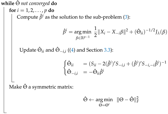
Our algorithm, called nsSLOPE, is summarized in Algorithm 1, which is essentially a block-coordinate descent algorithm [12,31]. Our algorithm may look similar to that of Yuan [19] but there are several important differences—(i) each sub-problem in our algorithm solves a SLOPE formulation (SL1 regularization), while Yuan’s sub-problem is either LASSO or Dantzig selector ( 1  regularization); (ii) our sub-problem makes use of the estimate Θ ^ i i in addition to Θ ^ i , i .
Algorithm 1: The nsSLOPE Algorithm
Input: X R n × p with zero-centered columns
Input: S = 1 n X X
Input: The target level of FDR q
 Set λ = ( λ 1 , , λ p 1 ) according to Section 3.2;
Symmetry 11 01311 i001

3.1. Sub-Problem Solver

To solve our sub-problems (3), we use the SLOPE R package, which implements the proximal gradient descent algorithm of Reference [32] with acceleration based on Nesterov’s original idea [33]. The algorithm requires to compute the proximal operator involving J λ ( · ) , namely
pro x J λ ( z ) : = arg   min x R p 1 1 2 x z 2 + J λ ( x ) .
This can be computed in O ( p log p ) time using an algorithm from Reference [21]. The optimality of sub-problem is declared by the primal-dual gap and we use a tight threshold value, 10 7 .

3.2. Choice of λ = ( λ 1 , , λ p 1 )

For the sequence of λ values in sub-problems, we use so-called the Benjamini-Hochberg (BH) sequence [21]:
λ i B H = Φ 1 ( 1 i q / 2 ( p 1 ) ) , i = 1 , , p 1 .
Here q [ 0 , 1 ] is the target level of FDR control we discuss later and Φ 1 ( α ) is the α th quantile of the standard normal distribution. In fact, when the design matrix X i in the SLOPE sub-problem (3) is not orthogonal, it is beneficial to use an adjusted version of this sequence. This sequence is generated by:
λ i = λ i B H 1 + w ( i 1 ) j < i λ j 2 , w ( k ) = 1 n k 1 ,
and if the sequence λ 1 , , λ k is non-increasing but λ i begins to increase after the index k , we set all the remaining values equal to λ k , so that the resulting sequence will be non-increasing. For more discussion about the adjustment, we refer to Section 3.2.2 of Reference [21].

3.3. Estimation of Θ i i

To solve the ith sub-problem in our algorithm, we need to estimate the value of Θ i i . This can be done using (4), that is, Θ i i = ( Σ i i ( β i ) Σ i , i β i ) 1 . However, this implies that (i) we need to keep an estimate of Σ R p × p additionally, (ii) the computation of the ith sub-problem will be dependent on all the other indices, as it needs to access Σ i , i , requiring the algorithm to run sequentially.
To avoid these overheads, we compute the estimate using the sample covariance matrix S = 1 n X X instead (we assume that the columns of X R n × p are centered):
Θ ˜ i i = ( S i i 2 β ^ S i , i + β ^ S i , i β ^ ) 1 .
This allows us to compute the inner loop of Algorithm 1 in parallel.

3.4. Stopping Criterion of the External Loop

To terminate the outer loop in Algorithm 1, we check if the diagonal entries of Θ ^ have converged, that is, the algorithm is stopped when the -norm different between two consecutive iterates is below a threshold value, 10 3 . The value is slightly loose but we have found no practical difference by making it tighter. Note that it is suffice to check the optimality of the diagonal entries of Θ ^ since the optimality of β ^ i ’s is enforced by the sub-problem solver and Θ ^ i , i = Θ ^ i i β ^ i .

3.5. Uniqueness of Sub-Problem Solutions

When p > n , our sub-problems may have multiple solutions, which may prevent the global convergence of our algorithm. We may adopt the technique in Reference [34] to inject a strongly convex proximity term into each sub-problem objective, so that each sub-problem will have a unique solution. In our experience, however, we encountered no convergence issues using stopping threshold values in the range of 10 3 10 7 for the outer loop.

4. Analysis

In this section, we provide two theoretical results of our nsSLOPE procedure—(i) an estimation error bound regarding the distance between our estimate Θ ˜ and the true model parameter Θ and (ii) group-wise FDR control on discovering the true edges in the Gaussian MRF corresponding to  Θ .
We first discuss about the estimation error bound, for which we divide our analysis into two parts regarding (i) off-diagonal entries and (ii) diagonal entries of  Θ .

4.1. Estimation Error Analysis

4.1.1. Off-Diagonal Entries

From (4), we see that β ^ i = Θ ^ i , i / Θ ^ i i , in other words, when Θ ^ i i is fixed, the off-diagonal entries Θ ^ i , i is determined solely by β ^ i , and therefore we can focus on the estimation error of β ^ i .
To discuss the estimation error of β ^ i , it is convenient to consider a constrained reformulation of the sub-problem (3):
β ^ arg   min β R d J λ ( β ) s . t . 1 n b A β 1 ϵ .
Hereafter, for the sake of simplicity, we use notations b : = X i R n and A : = X i R n × d for d : = p 1 , also dropping sub-problem indices in β ^ and ϵ > 0 . In this view, the data model being considered in each sub-problem is as follows,
b = A β + ν , ν N ( 0 , σ i 2 I n ) .
For the analysis, we make the following assumptions:
  • The true signal β R d satisfies β 1 s for some s > 0 (this condition is satisfied for example, if  β 2 1 and β is s-sparse, that is, it has at most s nonzero elements).
  • The noise satisfies the condition 1 n ν 1 ϵ . This will allow us to say that the true signal β is feasible with respect to the constraint in (6).
We provide the following result, which shows that β ^ approaches the true β in high probability:
Theorem 1.
Suppose that β ^ is an estimate of β obtained by solving the sub-problem (6). Consider the factorization A : = X i = B C where B R n × k ( n k ) is a Gaussian random matrix whose entries are sampled i.i.d. from N ( 0 , 1 ) and C R k × d is a deterministic matrix such that C C = Σ i , i . Such decomposition is possible since the rows of A are independent samples from N ( 0 , Σ i , i ) . Then we have,
β ^ β C 2 2 π 8 2 C 1 λ 1 λ ¯ s log k n + ϵ + t
with probability at least 1 2 exp n t 2 2 s λ ¯ 2 λ 1 2 , where λ ¯ = 1 d i = 1 d λ i and C 1 = max j = 1 , , d i = 1 k | C i j | .
We need to discuss a few results before proving Theorem 1.
Theorem 2.
Let T be a bounded subset of R d . For an ϵ > 0 , consider the set
T ϵ : = u T : 1 n A u 1 ϵ .
Then
sup u T ϵ ( u C C u ) 1 / 2 8 π n E sup u S | C g , u | + π 2 ( ϵ + t ) ,
holds with probability at least 1 2 exp n t 2 2 d ( T ) 2 , where g R k is a standard Gaussian random vector and d ( T ) : = max u T u 2 .
Proof. 
The result follows from an extended general M inequality in expectation [35]. □
The next result shows that the first term of the upper bound in Theorem 2 can be bounded without using expectation.
Lemma 1.
The quantity E sup u K K | C g , u | is called thewidthof K and is bounded as follows,
E sup u K K | C g , u | 4 2 C 1 λ 1 λ ¯ s log k .
Proof. 
This result is a part of the proof for Theorem 3.1 in Reference [35]. □
Using Theorem 2 and Lemma 1, we can derive a high probability error bound on the estimation from noisy observations,
b = A β + ν , 1 n ν 1 ϵ ,
where the true signal β belongs to a bounded subset K R d . The following corollaries are straightforward extensions of Theorems 3.3 and 3.4 of Reference [35], given our Theorem 2 (so we skip the proofs).
Corollary 1.
Choose β ^ to be any vector satisfying that
β ^ K , and 1 n b A β ^ 1 ϵ .
Then,
sup β K [ ( β ^ β ) C C ( β ^ β ) ] 1 / 2 2 π 8 2 C 1 λ 1 λ ¯ s log k n + ϵ + t
with probability at least 1 2 exp 2 n t 2 d ( T ) 2 .
Now we show the error bound for the estimates we obtain by solving the optimization problem (6). For the purpose, we make use of the Minkowski functional of the set K ,
β K : = inf { r > 0 : r β K }
If K R p is a compact and origin-symmetric convex set with non-empty interior, then · K defines a norm in R p . Note that β K if and only if β K 1 .
Corollary 2.
β ^ arg   min β R p β K subject to 1 n b A β 1 ϵ .
Then
sup β K [ ( β ^ β ) C C ( β ^ β ) ] 1 / 2 2 π 8 2 C 1 λ 1 λ ¯ s log k n + ϵ + t
with probability at least 1 2 exp 2 n t 2 d ( T ) 2 .
Finally, we show that solving the constrained form of the sub-problems (6) also satisfies essentially the same error bound in Corollary 2.
Proof of Theorem 1
Since we assumed that β 1 s , we construct the subset K so that all vectors β with β 1 s will be contained in K . That is,
K : = { β R p : J λ ( β ) λ 1 s } .
This is a sphere defined in the SL1-norm J λ ( · ) : in this case, the Minkowski functional · K is proportional to J λ ( · ) and thus the same solution minimizes both J λ ( · ) and · K .
Recall that d ( T ) : = max u T u 2 and we choose T = K K . Since β 2 β 1 1 λ ¯ J λ ( β ) , for  β K we have β 2 λ 1 λ ¯ s . This implies that d ( T ) = 2 λ 1 λ ¯ s . □

4.1.2. Diagonal Entries

We estimate Θ i i based on the residual sum of squares (RSS) as suggested by [19],
σ ^ i 2 = ( Θ ^ i i ) 1 = X i X i β ^ i 2 / n = S i i 2 ( β ^ i ) S i , i + ( β ^ i ) S i , i β ^ i .
Unlike in Reference [19], we directly analyze the estimation error of Θ ^ i i based on a chi-square tail bound.
Theorem 3.
For all small enough α > 0 so that α / σ i 2 [ 0 , 1 / 2 ) , we have
P ( | Θ ^ i i 1 Θ i i 1 δ ( ( β i ) , β ^ i ) | α ) exp 3 16 n α 2
where for ν N ( 0 , σ i 2 I n ) ,
δ ( β , β ^ ) : = ( β β ^ ) S i , i ( β β ^ ) + 2 ν X i ( β β ^ ) / n
Proof. 
Using the same notation as the previous section, that is, b = X i and A = X i , consider the estimate in discussion,
σ ^ i 2 = b A β ^ 2 / n = A ( β β ^ ) + ν 2 / n
where the last equality is from b = A β + ν . Therefore,
σ ^ i 2 = ( β β ^ ) S i , i ( β β ^ ) + 2 ν A ( β β ^ ) / n + ν ν / n
where S i , i : = A A / n = X i X i / n . The last term is the sum of squares of independent ν i N ( 0 , σ i 2 ) and therefore it follows the chi-square distribution, that is, ( ν ν ) / σ i 2 χ n 2 . Applying the tail bound [36] for a chi-square random variable Z with d degrees of freedom:
P ( | d 1 Z 1 | α ) exp 3 16 d α 2 , α [ 0 , 1 / 2 ) .
we get for all small enough α > 0 ,
P ( | ν ν / n σ i 2 | α ) exp 3 16 n α 2 .
 □

4.1.3. Discussion on Asymptotic Behaviors

Our two main results above, Theorems 1 and 3, indicate how well our estimate of the off-diagonal entries Θ ^ i , i and diagonal entries Θ ^ i i would behave. Based on these results, we can discuss the estimation error of the full matrix Θ ^ compared to the true precision matrix Θ .
From Theorem 1, we can deduce that with C C = Σ i , i and z ( n ) = O ( s log k / n ) ,
ev min ( Σ i , i ) β ^ β [ ( β ^ β ) Σ i , i ( β ^ β ) ] 1 / 2 2 π ( z ( n ) + ϵ + t )
where ev min ( Σ i , i ) is the smallest eigenvalue of the symmetric positive definite Σ i , i . That is, using the interlacing property of eigenvalues, we have
β ^ β 2 π ( z ( n ) + ϵ + t ) ev min ( Σ i , i ) 2 π Θ ( z ( n ) + ϵ + t )
where Θ = ev max ( Θ ) is the spectral radius of Θ . Therefore when n , the distance between β ^ and β is bounded by 2 π Θ ( ϵ + t ) . Here, we can consider t 0 in a way such as n t 2 as n increases, so that the bound in Theorem 1 will hold with the probability approaching one. That is, in rough asymptotics,
β ^ β ϵ 2 π Θ .
Under the conditions above, Theorem 3 indicates that:
δ ( β , β ^ ) S β β ^ 2 + 2 ν / n 1 X i ( β β ^ ) 2 ϵ 2 Θ ( π S Θ + 2 π X i )
using our assumption that ν / n 1 ϵ . We can further introduce assumptions on Θ and S Θ as in Reference [19], so that we can quantify the upper bound but here we will simply say that δ ( β , β ^ ) 2 c ϵ 2 , where c is a constant depending on the properties of the full matrices S and Θ . If this is the case, then from Theorem 3 for an α 0 such that n α 2 , we see that
| Θ ^ i i 1 Θ i i 1 | δ ( ( β i ) , β ^ i ) 2 c ϵ 2 ,
with the probability approaching one.
Therefore, if we can drive ϵ 0 as n , then (7) and (8) imply the convergence of the diagonal Θ ^ i i Θ i i and the off-diagonal Θ ^ i , i Θ i , i in probability. Since X i X i β 1 ϵ (or  X i X i β i ϵ i more precisely), ϵ 0 is likely to happen when ( p 1 ) / n 1 , implying that p as well as n .

4.2. Neighborhood FDR Control under Group Assumptions

Here we consider β ^ obtained by solving the unconstrained form (3) with the same data model we discussed above for the sub-problems:
b = A β + ν , ν N ( 0 , σ 2 I n )
with b = X i R n and A = X i R n × d with d = p 1 . Here we focus on a particular but an interesting case where the columns of A form orthogonal groups, that is, under the decomposition A = B C , C C = Σ i , i forms a block-diagonal matrix. We also assume that the columns of A belonging to the same group are highly correlated, in the sense that for any columns a i and a j of A corresponding to the same group, their correlation is high enough to satisfy that
a i a j min i = 1 , , d 1 { λ i λ i + 1 } / b .
This implies that β ^ i = β ^ j by Theorem 2.1 of Reference [25], which simplifies our analysis. Note that if a i and a j belong to different blocks, then our assumption above implies a i a j = 0 . Finally, we further assume that a i 1 for i = 1 , , d .
Consider a collection of non-overlapping index subsets g { 1 , , d } as the set of groups G. Under the block-diagonal covariance matrix assumption above, we see that
A β = g G i g a i β i = g G i g a i β g = g G a ˜ g a ˜ g β g
where β g denotes the representative of the same coefficients β i for all i g , a ˜ g : = i g a i and  β g : = a ˜ g β g . This tells us that we can replace A β by A ˜ β , if we define A ˜ R n × | G | containing a ˜ g a ˜ g in its columns (so that A ˜ A ˜ = I | G | ) and consider the vector of group-representative coefficients β R | G | .
The regularizer can be rewritten similarly,
J λ ( β ) = i = 1 | G | λ i | β | ( i ) = J λ ( β )
where λ i : = ( λ j = 1 i 1 | g ( j ) | + 1 + + λ j = 1 i | g ( i ) | ) / a ˜ g ( i ) , denoting by g ( i ) the group which has the ith largest coefficient in β in magnitude and by | g ( i ) | the size of the group.
Using the fact that A ˜ A ˜ = I | G | , we can recast the regression model (9) as b = A ˜ b = β + A ˜ ν N ( β , σ 2 I | G | ) , and consider a much simpler form of the problem (3),
β ^ = arg   min β R | G | 1 2 b β 2 + σ J λ ( β ) ,
where we can easily check that λ = ( λ 1 , , λ | G | ) satisfies λ 1 λ | G | . This is exactly the form of the SLOPE problem with an orthogonal design matrix in Reference [21], except that the new λ sequence is not exactly the Benjamini-Hochberg sequence (5).
We can consider the problem (3) (and respectively (10)) in the context of multiple hypothesis testing of d (resp. | G | ) null hypothesis H i : β i = 0 (resp. H g i : β i = 0 ) for i = 1 , , d (resp.  i = 1 , , | G | ), where we reject H i (resp. H g i ) if and only if β ^ i 0 (resp. β ^ i 0 ). In this setting, the Lemmas B.1 and B.2 in Reference [21] still holds for our problem (10), since they are independent of choosing the particular λ sequence.
In the following, V is the number of individual false rejections, R is the number of total individual rejections and R g is the number of total group rejections. The following lemmas are slightly modified versions of Lemmas B.1 and B.2 from Reference [21], respectively, to fit our group-wise setup.
Lemma 2.
Let H g be a null hypothesis and let r 1 . Then
{ b : H g is rejected R g = r } = { b : | b g | > σ λ r R g = r } .
Lemma 3.
Consider applying the procedure (10) for new data b ˜ = ( b 1 , , b g 1 , b g + 1 , , b | G | ) with λ ˜ = ( λ 2 , , λ d ) and let R ˜ g be the number of group rejections made. Then with r 1 ,
{ b : | b g | > σ λ r R g = r } { b : | b g | > σ λ r R ˜ g = r 1 } .
Using these, we can show our FDR control result.
Theorem 4.
Consider the procedure (10) we consider in a sub-problem of nsSLOPE as a multiple testing of group-wise hypotheses, where we reject the null group hypothesis H g : β g = 0 when β g 0 , rejecting all individual hypotheses in the group, that is, all H i , i g , are rejected. Using λ 1 , , λ p 1 defined as in (5), the procedure controls FDR at the level q [ 0 , 1 ] :
FDR = E V R 1 G 0 q d q
where
G 0 : = | { g : ( β g ) = 0 } | ( #   true   null   group   hypotheses ) V : = | { i : β i = 0 , β ^ i 0 } | ( #   false   ind .   rejections ) R : = | { i : β ^ i 0 } | ( #   all   individual   rejections )
Proof. 
Suppose that H g is rejected. Then,
P ( H g rejected R g = r ) ( i ) P ( | b g | σ λ r R ˜ g = r 1 ) = ( i i ) P ( | b g | σ λ r ) P ( R ˜ g = r 1 ) ( i i i ) P | b g | σ | g ( r ) | λ j = 1 r | g ( j ) | a ˜ g ( r ) P ( R ˜ g = r 1 ) ( i v ) P ( | b g | σ λ j = 1 r | g ( j ) | ) P ( R ˜ g = r 1 )
The derivations above are—(i) by using Lemmas 2 and 3; (ii) from the independence between b g and b ˜ ; (iii) by taking the smallest term in the summation of λ r multiplied by the number of terms; (iv) due to the assumption that a i 1 for all i, so that a ˜ g ( r ) | g ( r ) | by triangle inequality.
Now, consider the group-wise hypotheses testing in (10) is configured in a way that the first G 0 hypotheses are null in truth, that is, H g i : β i = 0 for i G 0 . Then we have:
FDR = E V R 1 = r = 1 | G | E V j = 1 r | g ( j ) | 1 { R g = r } = r = 1 | G | 1 j = 1 r | g ( j ) | i = 1 G 0 E [ 1 { H g i rejected } 1 { R g i = r } ] = r = 1 | G | 1 j = 1 r | g ( j ) | i = 1 G 0 P ( H g i rejected R g i = r ) r = 1 | G | 1 j = 1 r | g ( j ) | i = 1 G 0 j = 1 r | g ( j ) | q d P ( R ˜ g i = r 1 ) = r 1 q G 0 d P ( R ˜ g i = r 1 ) = q G 0 d q .
 □
Since the above theorem applies for each sub-problem, which can be considered as for the ith random variable to find its neighbors to be connected in the Gaussian Markov random field defined by Θ , we call this result as neighborhood FDR control.

5. Numerical Results

We show that the theoretical properties discussed above also works in simulated settings.

5.1. Quality of Estimation

For all numerical examples here, we generate n = 100 , 200 , 300 , 400 random i.i.d. samples from N ( 0 , Σ p × p ) , where p = 500 is fixed. We plant a simple block diagonal structure into the true matrix Σ , which is also preserved in the precision matrix Θ = Σ 1 . All the blocks had the same size of 4, so that we have total 125 blocks at the diagonal of Θ . We set Θ i i = 1 and set the entries Θ i j , i j , to a high enough value whenever ( i , j ) belongs to those blocks, in order to represent groups of highly correlated variables. All experiments were repeated for 25 times.
The λ sequence for nsSLOPE has been chosen according to Section 3.2 with respect to a target FDR level q = 0 . 05 . For the gLASSO, we have used the λ value discussed in Reference [3], to control the family-wise error rate (FWER, the chance of any false rejection of null hypotheses) to α = 0 . 05 .

5.1.1. Mean Square Estimation Error

Recall our discussion of error bounds in Theorem 1 (off-diagonal scaled by Θ ^ i i ) and Theorem 3 (diagonal), followed by Section 4.1.3 where we roughly sketched the asymptotic behaviors of Θ ^ i i and  Θ ^ i , i .
The top panel of Figure 1 shows mean square error (MSE) between estimated quantities and the true models that we have created, where estimates are obtained by our method nsSLOPE, without or with symmetrization at the end of Algorithm 1, as well as by the gLASSO  [4] which solves the 1 -based MLE problem (1) with a block coordinate descent strategy. The off-diagonal estimation was consistently good overall settings, while the estimation error of diagonal entries were kept improving as n is being increased, which was we predicted in Section 4.1.3. We believe that our estimation of the diagonal has room for improvement, for example, using more accurate reverse-scaling to compensate the normalization within the SLOPE procedure.

5.1.2. FDR Control

A more exciting part of our results is the FDR control discussed in Theorem 4 and here we check how well the sparsity structure of the precision matrix is recovered. For comparison, we measure the power (the fraction of the true nonzero entries discovered by the algorithm) and the FDR (for the whole precision matrix).
The bottom panel of Figure 1 shows the statistics. In all cases, the empirical FDR was controlled around the desired level 0 . 05 by all methods, although our method kept the level quite strictly, having significantly larger power than the gLASSO. This is understandable since FWER control of the gLASSO if often too respective, thereby limiting the power to detect true positive entries. It is also consistent with the results reported for SL1-based penalized regression [21,23], which indeed is one of the key benefits of SL1-based methods.

5.2. Structure Discovery

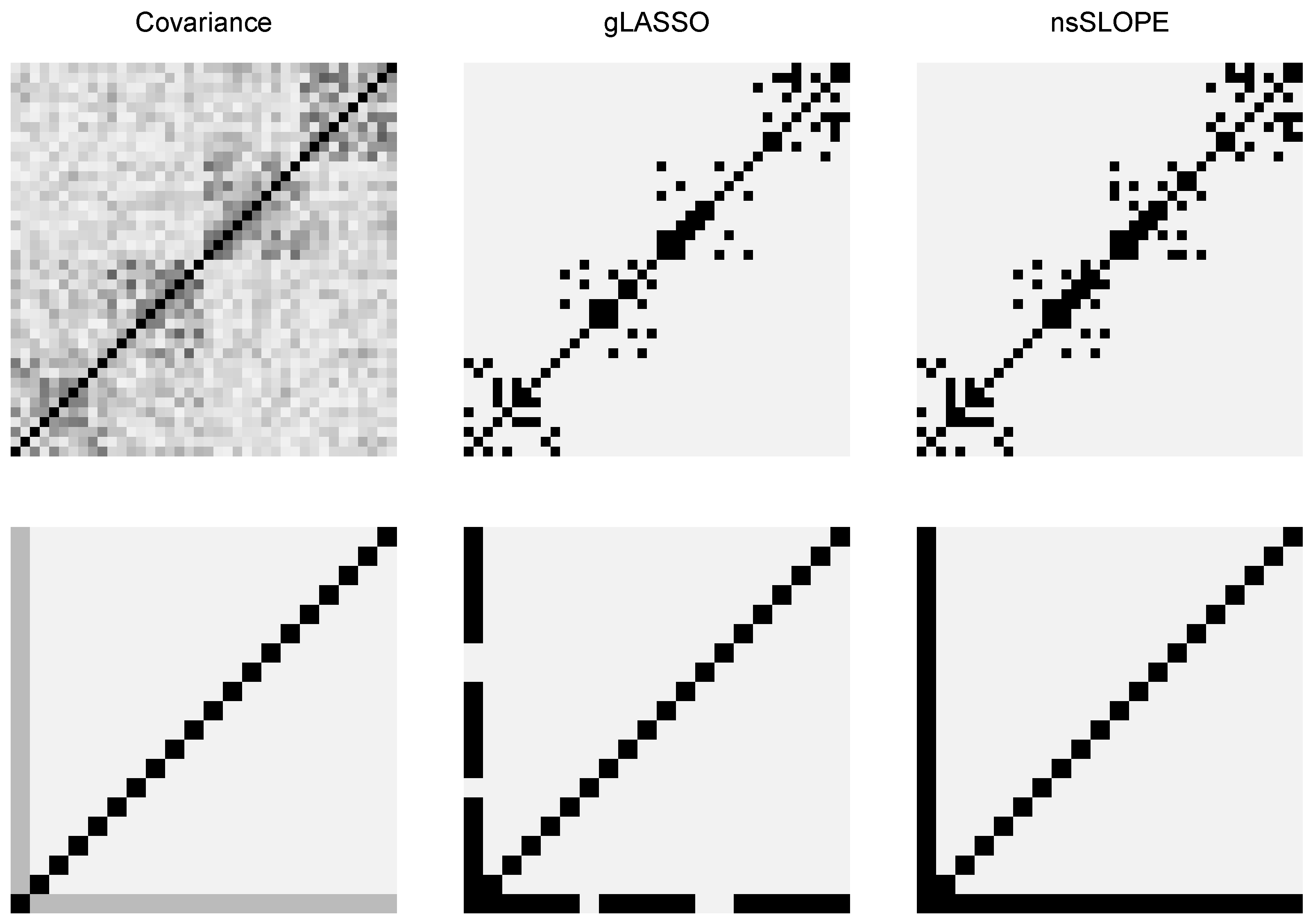
To further investigate the structure discovery by nsSLOPE, we have experimented with two different types of covariance matrices—one with a block-diagonal structure and another with a hub structure. The covariance matrix of the block diagonal case has been constructed using the data.simulation function from the varclust R package, with n = 100 , S N R = 1 , K = 4 , n u m b . v a r s = 10 , m a x . d i m = 3 (this gives us a data matrix with 100 examples and 40 variables). In the hub structure case, we have created a 20-dimensional covariance matrix with ones on the diagonal and 0 . 2 in the first column and the last row of the matrix. Then we have used the mvrnorm function from the MASS R package to sample 500 data points from a multivariate Gaussian distribution with zero mean and the constructed covariance matrix.
The true covariance matrix and the two estimates from gLASSO and nsSLOPE are shown in Figure 2. In nsSLOPE, the FDR control has been used based on the Benjamini-Hochberg sequence (5) with a target FDR value q = 0 . 05 and in gLASSO the FWER control [3] has been used with a target value α = 0 . 05 . Our method nsSLOPE appears to be more sensitive for finding the true structure, although it may contain a slightly more false discovery.

6. Conclusions

We introduced a new procedure based on the recently proposed sorted 1 regularization, to find solutions of sparse precision matrix estimation with more attractive statistical properties than the existing 1 -based frameworks. We believe there are many aspects of SL1 in graphical models to be investigated, especially when the inverse covariance has a more complex structure. Still, we hope our results will provide a basis for research and practical applications.
Our selection of the λ values in this paper requires independence assumptions on features or blocks of features. Although some extensions are possible [21], it would be desirable to consider a general framework, for example, based on Bayesian inference considering the posterior distribution derived from the loss and the regularizer [37,38], which enables us to evaluate the uncertainty of edge discovery and to find λ values from data.

Author Contributions

Conceptualization, S.L. and P.S.; methodology, S.L. and P.S.; software, S.L. and P.S.; validation, S.L, P.S. and M.B.; formal analysis, S.L.; writing–original draft preparation, S.L.; writing–review and editing, S.L.

Funding

This work was supported by the research fund of Hanyang University (HY-2018-N).

Conflicts of Interest

The authors declare no conflict of interest.

References

  1. Yuan, M.; Lin, Y. Model selection and estimation in the Gaussian graphical model. Biometrika 2007, 94, 19–35. [Google Scholar] [CrossRef] [Green Version]
  2. D’Aspremont, A.; Banerjee, O.; El Ghaoui, L. First-Order Methods for Sparse Covariance Selection. SIAM J. Matrix Anal. Appl. 2008, 30, 56–66. [Google Scholar] [CrossRef] [Green Version]
  3. Banerjee, O.; Ghaoui, L.E.; d’Aspremont, A. Model Selection Through Sparse Maximum Likelihood Estimation for Multivariate Gaussian or Binary Data. J. Mach. Learn. Res. 2008, 9, 485–516. [Google Scholar]
  4. Friedman, J.; Hastie, T.; Tibshirani, R. Sparse inverse covariance estimation with the graphical lasso. Biostatistics 2008, 9, 432–441. [Google Scholar] [CrossRef] [PubMed]
  5. Tibshirani, R. Regression Shrinkage and Selection via the Lasso. J. R. Stat. Soc. (Ser. B) 1996, 58, 267–288. [Google Scholar] [CrossRef]
  6. Oztoprak, F.; Nocedal, J.; Rennie, S.; Olsen, P.A. Newton-Like Methods for Sparse Inverse Covariance Estimation. In Advances in Neural Information Processing Systems 25; MIT Press: Cambridge, MA, USA, 2012; pp. 764–772. [Google Scholar]
  7. Rolfs, B.; Rajaratnam, B.; Guillot, D.; Wong, I.; Maleki, A. Iterative Thresholding Algorithm for Sparse Inverse Covariance Estimation. In Advances in Neural Information Processing Systems 25; MIT Press: Cambridge, MA, USA, 2012; pp. 1574–1582. [Google Scholar]
  8. Hsieh, C.J.; Dhillon, I.S.; Ravikumar, P.K.; Sustik, M.A. Sparse Inverse Covariance Matrix Estimation Using Quadratic Approximation. In Advances in Neural Information Processing Systems 24; MIT Press: Cambridge, MA, USA, 2011; pp. 2330–2338. [Google Scholar]
  9. Hsieh, C.J.; Banerjee, A.; Dhillon, I.S.; Ravikumar, P.K. A Divide-and-Conquer Method for Sparse Inverse Covariance Estimation. In Advances in Neural Information Processing Systems 25; MIT Press: Cambridge, MA, USA, 2012; pp. 2330–2338. [Google Scholar]
  10. Hsieh, C.J.; Sustik, M.A.; Dhillon, I.; Ravikumar, P.; Poldrack, R. BIG & QUIC: Sparse Inverse Covariance Estimation for a Million Variables. In Advances in Neural Information Processing Systems 26; MIT Press: Cambridge, MA, USA, 2013; pp. 3165–3173. [Google Scholar]
  11. Mazumder, R.; Hastie, T. Exact Covariance Thresholding into Connected Components for Large-scale Graphical Lasso. J. Mach. Learn. Res. 2012, 13, 781–794. [Google Scholar]
  12. Treister, E.; Turek, J.S. A Block-Coordinate Descent Approach for Large-scale Sparse Inverse Covariance Estimation. In Advances in Neural Information Processing Systems 27; MIT Press: Cambridge, MA, USA, 2014; pp. 927–935. [Google Scholar]
  13. Zhang, R.; Fattahi, S.; Sojoudi, S. Large-Scale Sparse Inverse Covariance Estimation via Thresholding and Max-Det Matrix Completion; International Conference on Machine Learning, PMLR: Stockholm, Sweden, 2018. [Google Scholar]
  14. Meinshausen, N.; Bühlmann, P. High-dimensional graphs and variable selection with the Lasso. Ann. Stat. 2006, 34, 1436–1462. [Google Scholar] [CrossRef] [Green Version]
  15. Meinshausen, N.; Bühlmann, P. Stability selection. J. R. Stat. Soc. (Ser. B) 2010, 72, 417–473. [Google Scholar] [CrossRef]
  16. Rothman, A.J.; Bickel, P.J.; Levina, E.; Zhu, J. Sparse permutation invariant covariance estimation. Electron. J. Stat. 2008, 2, 494–515. [Google Scholar] [CrossRef]
  17. Lam, C.; Fan, J. Sparsistency and rates of convergence in large covariance matrix estimation. Ann. Stat. 2009, 37, 4254–4278. [Google Scholar] [CrossRef]
  18. Raskutti, G.; Yu, B.; Wainwright, M.J.; Ravikumar, P.K. Model Selection in Gaussian Graphical Models: High-Dimensional Consistency of 1-regularized MLE. In Advances in Neural Information Processing Systems 21; MIT Press: Cambridge, MA, USA, 2009; pp. 1329–1336. [Google Scholar]
  19. Yuan, M. High Dimensional Inverse Covariance Matrix Estimation via Linear Programming. J. Mach. Learn. Res. 2010, 11, 2261–2286. [Google Scholar]
  20. Fattahi, S.; Zhang, R.Y.; Sojoudi, S. Sparse Inverse Covariance Estimation for Chordal Structures. In Proceedings of the 2018 European Control Conference (ECC), Limassol, Cyprus, 12–15 June 2018; pp. 837–844. [Google Scholar]
  21. Bogdan, M.; van den Berg, E.; Sabatti, C.; Su, W.; Candes, E.J. SLOPE—Adaptive Variable Selection via Convex Optimization. Ann. Appl. Stat. 2015, 9, 1103–1140. [Google Scholar] [CrossRef] [PubMed]
  22. Brzyski, D.; Su, W.; Bogdan, M. Group SLOPE—Adaptive selection of groups of predictors. arXiv 2015, arXiv:1511.09078. [Google Scholar] [CrossRef] [PubMed]
  23. Su, W.; Candès, E. SLOPE is adaptive to unknown sparsity and asymptotically minimax. Ann. Stat. 2016, 44, 1038–1068. [Google Scholar] [CrossRef]
  24. Bondell, H.D.; Reich, B.J. Simultaneous Regression Shrinkage, Variable Selection, and Supervised Clustering of Predictors with OSCAR. Biometrics 2008, 64, 115–123. [Google Scholar] [CrossRef]
  25. Figueiredo, M.A.T.; Nowak, R.D. Ordered Weighted L1 Regularized Regression with Strongly Correlated Covariates: Theoretical Aspects. In Proceedings of the 19th International Conference on Artificial Intelligence and Statistics, AISTATS 2016, Cadiz, Spain, 9–11 May 2016; pp. 930–938. [Google Scholar]
  26. Lee, S.; Brzyski, D.; Bogdan, M. Fast Saddle-Point Algorithm for Generalized Dantzig Selector and FDR Control with the Ordered l1-Norm. In Proceedings of the 19th International Conference on Artificial Intelligence and Statistics (AISTATS), Cadiz, Spain, 9–11 May 2016; Volume 51, pp. 780–789. [Google Scholar]
  27. Chen, S.; Banerjee, A. Structured Matrix Recovery via the Generalized Dantzig Selector. In Advances in Neural Information Processing Systems 29; Lee, D.D., Sugiyama, M., Luxburg, U.V., Guyon, I., Garnett, R., Eds.; Curran Associates, Inc.: Red Hook, NY, USA, 2016; pp. 3252–3260. [Google Scholar]
  28. Bellec, P.C.; Lecué, G.; Tsybakov, A.B. Slope meets Lasso: Improved oracle bounds and optimality. arXiv 2017, arXiv:1605.08651v3. [Google Scholar] [CrossRef]
  29. Derumigny, A. Improved bounds for Square-Root Lasso and Square-Root Slope. Electron. J. Stat. 2018, 12, 741–766. [Google Scholar] [CrossRef]
  30. Anderson, T.W. An Introduction to Multivariate Statistical Analysis; Wiley-Interscience: London, UK, 2003. [Google Scholar]
  31. Beck, A.; Tetruashvili, L. On the Convergence of Block Coordinate Descent Type Methods. SIAM J. Optim. 2013, 23, 2037–2060. [Google Scholar] [CrossRef]
  32. Beck, A.; Teboulle, M. A Fast Iterative Shrinkage-Thresholding Algorithm for Linear Inverse Problems. SIAM J. Imaging Sci. 2009, 2, 183–202. [Google Scholar] [CrossRef] [Green Version]
  33. Nesterov, Y. A Method of Solving a Convex Programming Problem with Convergence Rate O(1/k2). Soviet Math. Dokl. 1983, 27, 372–376. [Google Scholar]
  34. Razaviyayn, M.; Hong, M.; Luo, Z.Q. A Unified Convergence Analysis of Block Successive Minimization Methods for Nonsmooth Optimization. SIAM J. Optim. 2013, 23, 1126–1153. [Google Scholar] [CrossRef] [Green Version]
  35. Figueiredo, M.; Nowak, R. Sparse estimation with strongly correlated variables using ordered weighted 1 regularization. arXiv 2014, arXiv:1409.4005. [Google Scholar]
  36. Johnstone, I.M. Chi-square oracle inequalities. Lect. Notes-Monogr. Ser. 2001, 36, 399–418. [Google Scholar]
  37. Park, T.; Casella, G. The Bayesian Lasso. J. Am. Stat. Assoc. 2008, 103, 681–686. [Google Scholar] [CrossRef]
  38. Mallick, H.; Yi, N. A New Bayesian Lasso. Stat. Its Interface 2014, 7, 571–582. [Google Scholar] [CrossRef]
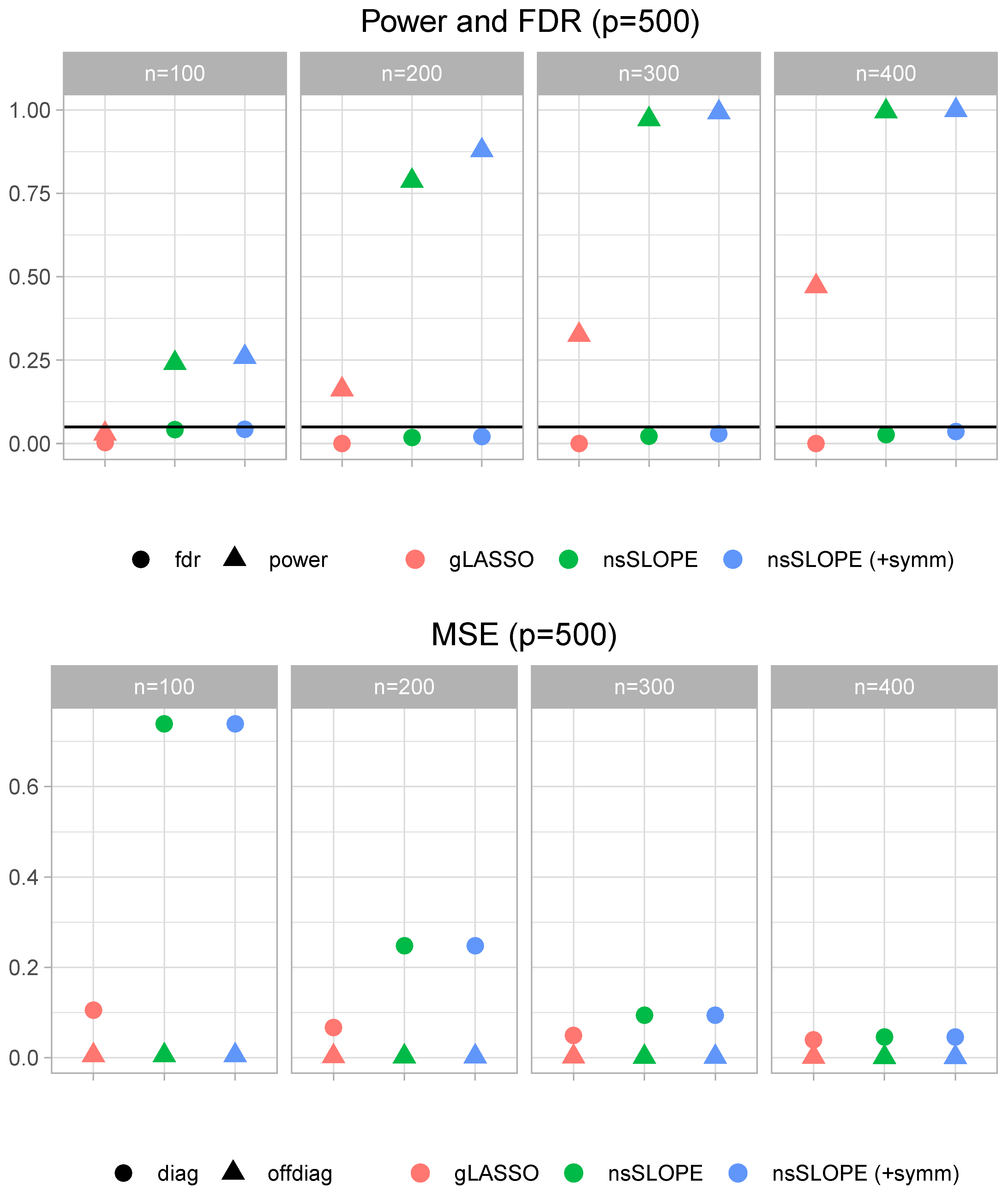
Figure 1. Quality of estimation. Top: empirical false discovery rate (FDR) levels (averaged over 25 repetitions) and the nominal level of q = 0 . 05 (solid black horizontal line). Bottom: mean square error of diagonal and off-diagonal entries of the precision matrix. p = 500 was fixed for both panels and n = 100 , 200, 300 and 400 were tried. (“nsSLOPE”: nsSLOPE without symmetrization, “+symm”: with symmetrization and gLASSO.)
Symmetry 11 01311 g001
Figure 2. Examples of structure discovery. Top: a covariance matrix with block diagonal structure. Bottom: a hub structure. True covariance matrix is shown on the left and gLASSO and nsSLOPE estimates (only the nonzero patterns) of the precision matrix are shown in the middle and in the right panels, respectively.
Symmetry 11 01311 g002