A Unified Proximity Algorithm with Adaptive Penalty for Nuclear Norm Minimization

Abstract

The nuclear norm minimization (NNM) problem is to recover a matrix that minimizes the sum of its singular values and satisfies some linear constraints simultaneously. The alternating direction method (ADM) has been used to solve this problem recently. However, the subproblems in ADM are usually not easily solvable when the linear mappings in the constraints are not identities. In this paper, we propose a proximity algorithm with adaptive penalty (PA-AP). First, we formulate the nuclear norm minimization problems into a unified model. To solve this model, we improve the ADM by adding a proximal term to the subproblems that are difficult to solve. An adaptive tactic on the proximity parameters is also put forward for acceleration. By employing subdifferentials and proximity operators, an equivalent fixed-point equation system is constructed, and we use this system to further prove the convergence of the proposed algorithm under certain conditions, e.g., the precondition matrix is symmetric positive definite. Finally, experimental results and comparisons with state-of-the-art methods, e.g., ADM, IADM-CG and IADM-BB, show that the proposed algorithm is effective.

1. Introduction

The rank minimization (RM) problem aims to recover an unknown low-rank matrix from very limited information. It has gained am increasing amount of attention rapidly in recent years, since it has a range of applications in many computer vision and machine learning areas, such as collaborative filtering [1], subspace segmentation [2], non-rigid structure from motion [3] and image inpainting [4]. This paper deals with the following rank minimization problem:

$$\underset{X\in {\mathbb{R}}^{m\times n}}{\min }\mathrm{rank}\left(X\right)\mathrm{s}.\mathrm{t}.\mathcal{A}X=\mathbf{b},$$

(1)

where $\mathcal{A}:{\mathbb{R}}^{m\times n}\to {\mathbb{R}}^p$ is a linear map and the vector $\mathbf{b}\in {\mathbb{R}}^p$ is known. The matrix completion (MC) problem is a special case of the RM problem, where $\mathcal{A}$ is a sampling operator in the form of $\mathcal{A}X=X_{\Omega }$, $\Omega \subset \{1,2,\dots ,m\}\times \{1,2,\dots ,n\}$ is an index subset, and $X_{\Omega }$ is a vector formed by the entries of X with indices in $\Omega$.

Although Label (1) is simple in form, directly solving it is an NP-hard problem due to the discrete nature of the rank function. One popular way is replacing the rank function with the nuclear norm, which is the sum of the singular values of a matrix. This technique is based on the fact that the nuclear norm minimization (NNM) is the tightest convex relaxation of the rank minimization problem [5]. The obtained new problem is given by

$$\underset{X\in {\mathbb{R}}^{m\times n}}{\min }{\parallel X\parallel }_{*}\mathrm{s}.\mathrm{t}.\mathcal{A}X=\mathbf{b},$$

(2)

where ${\parallel X\parallel }_{*}:={\sum }_{i=1}^r{\sigma }_i\left(X\right)$ denotes the nuclear norm. It has been shown that recovering a low-rank matrix can be achieved by solving Label (2) [1,6].

In practical applications, the observed data may be corrupted with noise, namely $b=\mathcal{A}X+e$, where e contains measurement errors dominated by certain normal distribution. In order to recover the low-rank matrix robustly, problem (2) should be modified to the following inequality constrained problem:

$$\underset{X\in {\mathbb{R}}^{m\times n}}{\min }{\parallel X\parallel }_{*}\mathrm{s}.\mathrm{t}.{\parallel \mathcal{A}X-\mathbf{b}\parallel }_2\le \delta ,$$

(3)

where ${\parallel ·\parallel }_2$ is the ${\ell }_2$ norm of vector and the constant $\delta \ge 0$ is the noise level. When $\delta =0$, problem (3) reduces to the noiseless case (2).

Alternatively, problems (2) and (3) can be rewritten as the nuclear norm regularized least-square (NNRLS) under some conditions:

$$\underset{X\in {\mathbb{R}}^{m\times n}}{\min }{\parallel X\parallel }_{*}+\frac{\gamma }{2}{\parallel \mathcal{A}X-\mathbf{b}\parallel }_2^2,$$

(4)

where $\gamma >0$ is as given parameter.

The studies on the nuclear norm minimization problem are mainly along two directions. The first one is enhancing the precision of a low rank approximation via replacing the nuclear norm by a non-convex regularizer—for instance, the Schatten p-norm [7,8], the truncated nuclear norm [4,9], the log or fraction function based norm [10,11], and so on. The second one is improving the efficiency of solving problems (2), (3) and (4) and their variants. For instance, the authors in [12] treated the problem (2) as a standard linear semidefinite programming (SDP) problem, and proposed the solving algorithm from the dual problem. However, since the SDP solver uses second-order information, with the increase in the size of the matrix, the memory required to calculate the descending direction quickly becomes too large. Therefore, algorithms that use only first-order information are developed, such as the singular value thresholding (SVT) algorithm [13], the fixed point continuation algorithm (FPCA) [14], the accelerated proximal gradient Lagrangian (APGL) method [15], the proximal point algorithm based on indicator function (PPA-IF) [16], the augmented Lagrange multiplier (ALM) algorithm [17] and the alternating direction methods (ADM) [18,19,20,21].

In particular, Chen et al. [18] applied the ADM to solve the nuclear norm based matrix completion problem. Due to the simplicity of the linear mapping $\mathcal{A}$, i.e., $\mathcal{A}{\mathcal{A}}^{*}=\mathcal{I}$, all of the ADM subproblems of the matrix completion problem can be solved exactly by an explicit formula; see [18] for details. Here, and hereafter ${\mathcal{A}}^{*}$ and $\mathcal{I}$ represent the adjoint of $\mathcal{A}$ and the identity operator. However, for a generic $\mathcal{A}$ with $\mathcal{A}{\mathcal{A}}^{*}\ne \mathcal{I}$, some of the resulting subproblems no longer have closed-form solutions. Thus, the efficiency of the ADM depends heavily on how to solve these harder subproblems.

To solve this difficulty, a common strategy is to introduce new auxiliary variables, e.g., in [19], one auxiliary variable was introduced for solving Label (2), while two auxiliary variables were introduced for Label (3). However, with more variables and more constraints, more memory is required and the convergence of ADM also becomes slower. Moreover, to update auxiliary variables, whose subproblems are least square problems, expensive matrix inversions are often necessary. Even worse, the convergence of ADM with more than two variables is not guaranteed. To mitigate these problems, Yang and Yuan [21] presented a linearized ADM to solve the NNRLS (4) as well as problems (2) and (3), where each subproblems admit explicit solutions. Instead of the linearized technique, Xiao and Jin [19] solve one least square subproblem iteratively by the Barzilai–Borwein (BB) gradient method [22]. Unlike [19], Jin et al. [20] used the linear conjugate gradient (CG) algorithm rather than BB to solve the subproblem.

In this paper, we further investigate the efficiency of ADM in solving the nuclear norm minimization problems. We first reformulate the problems (2), (3) and (4) into a unified form as follows:

$$\underset{X\in {\mathbb{R}}^{m\times n}}{\min }f\left(X\right)+g\left(\mathcal{A}X\right),$$

(5)

where $f:{\mathbb{R}}^{m\times n}\to \mathbb{R}$ and $g:{\mathbb{R}}^p\to \mathbb{R}$. In this paper, we always fix $f(·)={\parallel ·\parallel }_{*}$. When considering problems (2) and (3), we choose $g(·)={\mathcal{X}}_{B_{\delta }}(·-\mathbf{b})$, where ${\mathcal{X}}_{B_{\delta }}(·)$ denotes the indicator function over $B_{\delta }:=\{\mathbf{u}\in {\mathbb{R}}^p\mid {\parallel \mathbf{u}\parallel }_2\le \delta \}$, i.e.,

$$\begin{array}{c}\hfill {\mathcal{X}}_{B_{\delta }}\left(\mathbf{x}\right):=\left\{\begin{array}{cc}0,\hfill & \mathrm{if}\mathbf{x}\in B_{\delta },\hfill \\ +\infty ,\hfill & \mathrm{otherwise}.\hfill \end{array}\right.\end{array}$$

(6)

When considering problem (4), we choose $g(·)=\frac{\gamma }{2}{\parallel ·-\mathbf{b}\Vert }_2^2$. As a result, for a general linear mapping $\mathcal{A}$, we only need to solve such a problem whose objective function is a sum of two convex functions and one of them contains an affine transformation.

Motivated by the ADM algorithms above, we then present a unified proximity algorithm with adaptive penalty (PA-AP) to solve Label (5). In particular, we employ the proximity idea to deal with the problems encountered by the present ADM, by adding a proximity term to one of the subproblems. We term the proposed algorithm as a proximity algorithm because we can rewrite it as a fixed-point equation system of proximity operators of f and g. By analyzing the fixed-point equations and applying the “Condition-M” [23], the convergence of the algorithm is proved under some assumptions. Furthermore, to improve the efficiency, an adaptive tactic on the proximity parameters is put forward. This paper is closely related to the works [23,24,25,26]. However, this paper is motivated to improve ADM to solve the nuclear norm minimization problem with linear affine constraints.

The organization of this paper is as follows. In Section 2, a review of ADM and its application on NNM are provided. In addition, the properties about subdifferentials and proximity operators are introduced. To improve ADM, a proximity algorithm with adaptive penalty is proposed, and convergence of the proposed algorithm is obtained in Section 3. Section 4 demonstrates the performance and effectiveness of the algorithm through numerical experiment. Finally, we will make a conclusion in Section 5.

2. Preliminaries

In this section, we give a brief review on ADM and its applications to the NNM problem (2) developed in [19,20]. In addition, some preliminaries on subdifferentials and proximity operators are given. Throughout this paper, linear maps are denoted with calligraphic letters (e.g., $\mathcal{A}$), while capital letters represent matrices (e.g., A), and boldface lowercase letters represent vectors (e.g., $\mathbf{x}$).

We begin with introducing the ADM. The basic idea of ADM goes back to the work of Gabay and Mercier [27]. ADM is designed to solving the separable convex minimization problem:

$$\underset{\mathbf{x},\mathbf{y}}{\min }{\theta }_1\left(\mathbf{x}\right)+{\theta }_2\left(\mathbf{y}\right),\mathrm{s}.\mathrm{t}.A\mathbf{x}+B\mathbf{y}=\mathbf{c},$$

(7)

where ${\theta }_1:{\mathbb{R}}^s\to \mathbb{R}$, ${\theta }_2:{\mathbb{R}}^t\to \mathbb{R}$ are convex functions, and $A\in {\mathbb{R}}^{l\times s}$, $B\in {\mathbb{R}}^{l\times t}$ and $\mathbf{c}\in {\mathbb{R}}^l$. The corresponding augmented Lagrangian function is

$$\mathcal{L}(\mathbf{x},\mathbf{y},\lambda )={\theta }_1\left(\mathbf{x}\right)+{\theta }_2\left(\mathbf{y}\right)-⟨\lambda ,A\mathbf{x}+B\mathbf{y}-\mathbf{c}⟩+\frac{\beta }{2}{\parallel A\mathbf{x}+B\mathbf{y}-\mathbf{c}\parallel }_2^2,$$

(8)

where $\lambda \in {\mathbb{R}}^l$ is the Lagrangian multiplier and $\beta >0$ is a penalty parameter. ADM is to minimize (8) first with respect to $\mathbf{x}$, then with respect to $\mathbf{y}$, and finally update $\lambda$ iteratively, i.e.,

$$\begin{array}{c}\hfill \left\{\begin{array}{c}{\mathbf{x}}_{k+1}=\arg \underset{\mathbf{x}}{\min }\mathcal{L}(\mathbf{x},{\mathbf{y}}_k,{\lambda }_k),\hfill \\ {\mathbf{y}}_{k+1}=\arg \underset{\mathbf{y}}{\min }\mathcal{L}({\mathbf{x}}_{k+1},\mathbf{y},{\lambda }_k),\hfill \\ {\lambda }_{k+1}={\lambda }_k-\beta (A{\mathbf{x}}_{k+1}+B{\mathbf{y}}_{k+1}-\mathbf{c}).\hfill \end{array}\right.\end{array}$$

(9)

The main advantage of ADM is to make use of the separability structure of the objective function ${\theta }_1\left(\mathbf{x}\right)+{\theta }_2\left(\mathbf{y}\right)$.

To solve (2) based on ADM, the authors in [19,20] introduced an auxiliary variable Y, and equivalently transformed the original model into

$$\underset{X,Y}{\min }{\parallel X\parallel }_{*}\mathrm{s}.\mathrm{t}.X-Y=0,\mathcal{A}Y=\mathbf{b}.$$

(10)

The augmented Lagrangian function to (10) is

$$\mathcal{L}(X,Y,Z,\mathbf{z})={\parallel X\parallel }_{*}-⟨Z,X-Y⟩+\frac{\mu }{2}{\parallel X-Y\parallel }_F^2-⟨\mathbf{z},\mathcal{A}Y-\mathbf{b}⟩+\frac{\gamma }{2}{\parallel \mathcal{A}Y-\mathbf{b}\parallel }_2^2,$$

(11)

where $Z\in {\mathbb{R}}^{m\times n}$, $\mathbf{z}\in {\mathbb{R}}^p$ are Lagrangian multipliers, $\mu ,\gamma >0$ are penalty parameters and $⟨·⟩$ denotes the Frobenius inner product, i.e., the matrices are treated like vectors. Following the idea of ADM, given $(X_k,Y_k)$, the next pair $(X_{k+1},Y_{k+1})$ is determined by alternating minimizing (11),

$$\begin{array}{c}\hfill \left\{\begin{array}{c}{X}_{k+1}=\arg \underset{X}{\min }\mathcal{L}(X,Y_k,Z_k,{\mathbf{z}}_k),\hfill \\ Y_{k+1}=\arg \underset{Y}{\min }\mathcal{L}(X_{k+1},Y,Z_k,{\mathbf{z}}_k),\hfill \\ Z_{k+1}=Z_k-\mu (X_{k+1}-Y_{k+1}),\hfill \\ {\mathbf{z}}_{k+1}={\mathbf{z}}_k-\gamma (\mathcal{A}{Y}_{k+1}-\mathbf{b}).\hfill \end{array}\right.\end{array}$$

(12)

Firstly, $X_{k+1}$ can be updated by

$$\begin{array}{ccc}\hfill X_{k+1}& =& \arg \underset{X}{\min }{\parallel X\parallel }_{*}-⟨Z_k,X-Y_k⟩+\frac{\mu }{2}{\parallel X-Y_k\parallel }_F^2\hfill \\ & =& \arg \underset{X}{\min }{\parallel X\parallel }_{*}+\frac{\mu }{2}{\parallel X-(Y_k+\frac{1}{\mu }{Z}_k)\parallel }_F^2,\hfill \end{array}$$

(13)

which in fact corresponds to evaluating the proximal operator of ${\parallel ·\parallel }_{*}$, i.e., ${\mathrm{prox}}_{\frac{1}{\beta }{\parallel ·\parallel }_{*}}$ which is defined below.

Secondly, given $(X_{k+1},Z_k,{\mathbf{z}}_k)$, $Y_{k+1}$ can be updated by

$$\begin{array}{ccc}\hfill Y_{k+1}& =& \arg \underset{Y}{\min }-⟨Z_k,X_{k+1}-Y⟩+\frac{\mu }{2}\parallel X_{k+1}{-Y\parallel }_F^2-⟨{\mathbf{z}}_k,\mathcal{A}Y-b⟩+\frac{\gamma }{2}{\parallel \mathcal{A}Y-\mathbf{b}\parallel }_2^2\hfill \\ & =& \arg \underset{Y}{\min }\frac{\mu }{2}\parallel Y-(X_{k+1}-\frac{1}{\mu }{Z}_k){\parallel }_F^2+\frac{\gamma }{2}{\parallel \mathcal{A}Y-(\mathbf{b}+\frac{1}{\gamma }{\mathbf{z}}_k)\parallel }_2^2,\hfill \end{array}$$

(14)

which is a least square subproblem. Its solution can be found by solving a linear equation:

$$(\mu \mathcal{I}+\gamma {\mathcal{A}}^{*}\mathcal{A})Y=\mu X_{k+1}-Z_k-{\mathcal{A}}^{*}(\gamma \mathbf{b}+{\mathbf{z}}_k).$$

However, computing the matrix inverse ${(\mu \mathcal{I}+\gamma {\mathcal{A}}^{*}\mathcal{A})}^{-1}$ is too costly to implement. Though [19,20] adopted inverse-free methods, i.e., BB and CG, to solve (14) iteratively, they are still inefficient, which will be shown in Section 4.

Next, we review definitions of subdifferential and proximity operator, which play an important role in the algorithm and convergence analysis. The subdifferential of a convex function $\theta$ at a point $\mathbf{x}\in {\mathbb{R}}^d$ is the set defined by

$${\partial }_{\theta (·)}\left(\mathbf{x}\right)=\{\mathbf{y}\in {\mathbb{R}}^d:\theta \left(\mathbf{z}\right)\ge \theta \left(\mathbf{x}\right)+<\mathbf{y},\mathbf{z}-\mathbf{x}>,\forall \mathbf{z}\in {\mathbb{R}}^d\}.$$

(15)

The conjugate function of $\theta$ is denoted by ${\theta }^{*}$, which is defined by

$${\theta }^{*}\left(\mathbf{y}\right):=\underset{\mathbf{x}}{sup}\{⟨\mathbf{x},\mathbf{y}⟩-\theta \left(\mathbf{x}\right)\}.$$

For $\mathbf{x}\in \mathrm{dom}\left(\theta \right)$, $\mathbf{y}\in \mathrm{dom}\left({\theta }^{*}\right)$, it holds that

$$\mathbf{y}\in {\partial }_{\theta (·)}\left(\mathbf{x}\right)\iff \mathbf{x}\in {\partial }_{{\theta }^{*}(·)}\left(\mathbf{y}\right),$$

(16)

where $\mathrm{dom}(·)$ denotes the domain of a function.

For a given positive definite matrix $\mathcal{H}$, the weighted inner product is defined by ${⟨\mathbf{x},\mathbf{y}⟩}_{\mathcal{H}}=⟨\mathcal{H}\mathbf{x},\mathbf{y}⟩$. Furthermore, the proximity operator of $\theta$ at $\mathbf{x}$ with respect to $\mathcal{H}$ [23] is defined by

$${\mathrm{prox}}_{\theta (·),\mathcal{H}}\left(\mathbf{x}\right)=\arg \min \{\theta \left(\mathbf{u}\right)+\frac{1}{2}{\parallel \mathbf{u}-\mathbf{x}\parallel }_{\mathcal{H}}^2:\mathbf{u}\in {\mathbb{R}}^d\}.$$

(17)

If $\mathcal{H}=\beta \mathcal{I}$, then ${\mathrm{prox}}_{\theta (·),\mathcal{H}}(·)$ is reduced to

$${\mathrm{prox}}_{\theta (·),\beta \mathcal{I}}\left(\mathbf{x}\right)=\arg \min \{\theta \left(\mathbf{u}\right)+\frac{\beta }{2}{\parallel \mathbf{u}-\mathbf{x}\parallel }_2^2:\mathbf{u}\in {\mathbb{R}}^d\},$$

and ${\mathrm{prox}}_{\frac{1}{\beta }\theta (·)}(·)$ is short for ${\mathrm{prox}}_{\theta (·),\beta \mathcal{I}}(·)$. A relation between subdifferentials and proximity operators is that

$$\mathbf{y}\in {\partial }_{\theta (·)}\left(\mathbf{x}\right)\iff \mathbf{x}={\mathrm{prox}}_{\theta (·)}(\mathbf{x}+\mathbf{y}),$$

(18)

which is frequently used to construct fixed-point equations and prove convergence of the algorithm.

3. Proximity Algorithm with Adaptive Penalty

In Section 2, it is shown that the current ADM results in expensive matrix inverse computation when solving (2). Therefore, it is desirable to improve it. In this section, we propose a proximity algorithm with adaptive penalty (PA-AP) to solve the unified problem (5).

3.1. Proximity Algorithm

We derive our algorithm from ADM. First of all, we introduce an auxiliary variable $\mathbf{y}\in {\mathbb{R}}^p$, and convert (5) to

$$\underset{X,\mathbf{y}}{\min }f\left(X\right)+g\left(\mathbf{y}\right),\mathrm{s}.\mathrm{t}.\mathcal{A}X-\mathbf{y}=0.$$

(19)

The augmented Lagrangian function of (19) is defined by

$$\mathcal{L}(X,\mathbf{y})=f\left(X\right)+g\left(\mathbf{y}\right)-⟨\lambda ,\mathcal{A}X-\mathbf{y}⟩+\frac{\mu }{2}{\parallel \mathcal{A}X-\mathbf{y}\parallel }_2^2,$$

(20)

where $\lambda \in {\mathbb{R}}^p$ is the Lagrangian multiplier and $\mu >0$ is a penalty parameter. ADM first updates X by minimizing $\mathcal{L}(X,\mathbf{y})$ with $\mathbf{y}$ being fixed and then updates $\mathbf{y}$ with X fixed at its latest value, until some convergence criteria are satisfied. After some simplification, we get

$$\begin{array}{c}\hfill \left\{\begin{array}{c}{X}_{k+1}=\arg \underset{X}{\min }f\left(X\right)+\frac{\mu }{2}{\parallel \mathcal{A}X-({\mathbf{y}}_k+\frac{1}{\mu }{\lambda }_k)\parallel }_2^2,\hfill \\ {\mathbf{y}}_{k+1}=\arg \underset{\mathbf{y}}{\min }g\left(\mathbf{y}\right)+\frac{\mu }{2}{\parallel \mathbf{y}-(\mathcal{A}{X}_{k+1}-\frac{1}{\mu }{\lambda }_k)\parallel }_2^2,\hfill \\ {\lambda }_{k+1}={\lambda }_k-\mu (\mathcal{A}{X}_{k+1}-{\mathbf{y}}_{k+1}).\hfill \end{array}\right.\end{array}$$

(21)

Note that the subproblem of $X_{k+1}$ usually has no closed-form solutions when $\mathcal{A}$ is not the identity. In order to design efficient algorithms, we add a proximity term to this subproblem. More precisely, we propose the following algorithm:

$$\begin{array}{c}\hfill \left\{\begin{array}{c}{X}_{k+1}=\arg \underset{X}{\min }f\left(X\right)+\frac{\mu }{2}\parallel \mathcal{A}X-({\mathbf{y}}_k+\frac{1}{\mu }{\lambda }_k){\parallel }_2^2+\frac{1}{2}{\parallel X-X_k\parallel }_Q^2,\hfill \\ {\mathbf{y}}_{k+1}=\arg \underset{\mathbf{y}}{\min }g\left(\mathbf{y}\right)+\frac{\mu }{2}{\parallel \mathbf{y}-(\mathcal{A}{X}_{k+1}-\frac{1}{\mu }{\lambda }_k)\parallel }_2^2,\hfill \\ {\lambda }_{k+1}={\lambda }_k-\mu (\mathcal{A}{X}_{k+1}-{\mathbf{y}}_{k+1}),\hfill \end{array}\right.\end{array}$$

(22)

where $Q\in {\mathbb{R}}^{m\times m}$ is a symmetric positive definite matrix.

The next lemma shows that (22) is equivalent to a fixed-point equation of some proximity operators. The proof is similar to [25].

Lemma 1.

The problem (22) is equivalent to solving the following equations:

$$\begin{array}{c}\hfill \left\{\begin{array}{c}{\mathbf{z}}_{k+1}={\mathrm{prox}}_{\mu g^{*}(·)}(\mu \mathcal{A}{X}_k+{\mathbf{z}}_k),\hfill \\ X_{k+1}={\mathrm{prox}}_{\tau f(·)}(X_{k+1}-\tau (\mu {\mathcal{A}}^{*}\mathcal{A}+Q)(X_{k+1}-X_k)-\tau {\mathcal{A}}^{*}(2{\mathbf{z}}_{k+1}-{\mathbf{z}}_k)),\hfill \end{array}\right.\end{array}$$

(23)

where $\tau >0$ is arbitrary.

Proof. 

By changing the order of iterations, the first-order optimality condition of (22) is

$$\begin{array}{c}\hfill \left\{\begin{array}{c}0\in {\partial }_{g(·)}\left({\mathbf{y}}_{k+1}\right)+\mu ({\mathbf{y}}_{k+1}-\mathcal{A}{X}_k+\frac{1}{\mu }{\lambda }_k),\hfill \\ {\lambda }_{k+1}={\lambda }_k-\mu (\mathcal{A}{X}_k-{\mathbf{y}}_{k+1}),\hfill \\ 0\in {\partial }_{f(·)}\left(X_{k+1}\right)+\mu {\mathcal{A}}^{*}(\mathcal{A}{X}_{k+1}-{\mathbf{y}}_{k+1}-\frac{1}{\mu }{\lambda }_{k+1})+Q(X_{k+1}-X_k).\hfill \end{array}\right.\end{array}$$

(24)

From the first line of (24) and (16), we obtain

$$\mu {\mathbf{y}}_{k+1}\in {\partial }_{\mu g^{*}(·)}(\mu (\mathcal{A}{X}_k-{\mathbf{y}}_{k+1})-{\lambda }_k).$$

(25)

Denote ${\mathbf{z}}_k:=-{\lambda }_k$. Then,

$${\mathbf{z}}_{k+1}=\mu \mathcal{A}{X}_k+{\mathbf{z}}_k-\mu {\mathbf{y}}_{k+1}.$$

(26)

Using (18), it follows from (25) and (26) that

$${\mathbf{z}}_{k+1}={\mathrm{prox}}_{\mu g^{*}(·)}(\mu \mathcal{A}{X}_k+{\mathbf{z}}_k).$$

(27)

By (26), we have

$$\mu \mathcal{A}{X}_k+{\mathbf{z}}_k=\mu {\mathbf{y}}_{k+1}+\mu (\mathcal{A}{X}_k-{\mathbf{y}}_{k+1}-\frac{1}{\mu }{\lambda }_k)=\mu {\mathbf{y}}_{k+1}+{\mathbf{z}}_{k+1},$$

and thus

$$\mu {\mathcal{A}}^{*}(\mathcal{A}{X}_{k+1}-{\mathbf{y}}_{k+1}-\frac{1}{\mu }{\lambda }_{k+1})+Q(X_{k+1}-X_k)=(\mu {\mathcal{A}}^{*}\mathcal{A}+Q)(X_{k+1}-X_k)+{\mathcal{A}}^{*}(2{\mathbf{z}}_{k+1}-{\mathbf{z}}_k).$$

(28)

From (28) and the third line of (24), given $\tau >0$, we have

$$-\tau (\mu {\mathcal{A}}^{*}\mathcal{A}+Q)(X_{k+1}-X_k)-\tau {\mathcal{A}}^{*}(2{\mathbf{z}}_{k+1}-{\mathbf{z}}_k)\in {\partial }_{\tau f(·)}\left(X_{k+1}\right),$$

which yields

$$X_{k+1}={\mathrm{prox}}_{\tau f(·)}(X_{k+1}-\tau (\mu {\mathcal{A}}^{*}\mathcal{A}+Q)(X_{k+1}-X_k)-\tau {\mathcal{A}}^{*}(2{\mathbf{z}}_{k+1}-{\mathbf{z}}_k)).$$

(29)

Therefore, the results in (23) are achieved by combining (27) and (29). □

We now discuss the choice of Q. To make the first subproblem of (22) have closed-form solutions, in this paper, we simply choose $Q=\mu \eta \mathcal{I}-\mu {\mathcal{A}}^{*}\mathcal{A}$. To make sure Q is positive definite, $\eta$ must satisfy ${\eta >\parallel \mathcal{A}\parallel }_2^2$, where ${\parallel ·\parallel }_2$ is the spectral norm. By substituting Q into (22), we obtain

$$\begin{array}{c}\hfill \left\{\begin{array}{c}{X}_{k+1}=\arg \underset{X}{\min }f\left(X\right)+\frac{\mu \eta }{2}{\parallel X-(X_k+\frac{{\mathcal{A}}^{*}({\lambda }_k-\mu (\mathcal{A}{X}_k-{\mathbf{y}}_k))}{\mu \eta })\parallel }_2^2,\hfill \\ {\mathbf{y}}_{k+1}=\arg \underset{\mathbf{y}}{\min }g\left(\mathbf{y}\right)+\frac{\mu }{2}{\parallel \mathbf{y}-(\mathcal{A}{X}_{k+1}-\frac{1}{\mu }{\lambda }_k)\parallel }_2^2,\hfill \\ {\lambda }_{k+1}={\lambda }_k-\mu (\mathcal{A}{X}_{k+1}-{\mathbf{y}}_{k+1}).\hfill \end{array}\right.\end{array}$$

(30)

The subproblems in (30) can be solved explicitly based on proximity operators. Specifically, we have

$$X_{k+1}={\mathrm{prox}}_{\frac{1}{\mu \eta }{\parallel ·\parallel }_{*}}(X_k+\frac{{\mathcal{A}}^{*}({\lambda }_k-\mu (\mathcal{A}{X}_k-{\mathbf{y}}_k))}{\mu \eta })=Umax\{\Sigma -\frac{1}{\mu \eta },0\}{V}^T,$$

(31)

where $U\Sigma V^T$ is the singular value decomposition (SVD) of $X_k+\frac{{\mathcal{A}}^{*}({\lambda }_k-\mu (\mathcal{A}{X}_k-{\mathbf{y}}_k))}{\mu \eta }$, $U\in {\mathbb{R}}^{m\times m}$, $V\in {\mathbb{R}}^{n\times n}$, and $\Sigma \in {\mathbb{R}}^{m\times n}$ is a diagonal matrix containing the singular values.

Moreover, ${\mathbf{y}}_{k+1}={\mathrm{prox}}_{\frac{1}{\mu }g(·)}(\mathcal{A}{X}_{k+1}-\frac{1}{\mu }{\lambda }_k)$, which depends on the choice of $g(·)$. If $g(·)={\mathcal{X}}_{B_{\delta }}(·-\mathbf{b})$, then

$$\begin{array}{c}\hfill pro{x}_{\frac{1}{\mu }g(·)}\left(\mathbf{x}\right)=\left\{\begin{array}{cc}\mathbf{x},\hfill & \mathbf{x}-\mathbf{b}\in B_{\delta },\hfill \\ \mathbf{b}+\frac{\delta }{{\parallel \mathbf{x}-\mathbf{b}\parallel }_2}(\mathbf{x}-\mathbf{b}),\hfill & otherwise.\hfill \end{array}\right.\end{array}$$

(32)

If $g\left(\mathbf{x}\right)=\frac{\gamma }{2}{\parallel \mathbf{x}-\mathbf{b}\parallel }_2^2$, then

$$pro{x}_{\frac{1}{\mu }g(·)}\left(\mathbf{x}\right)=\frac{\gamma \mathbf{b}+\mu \mathbf{x}}{\gamma +\mu }.$$

(33)

3.2. Adaptive Penalty

In previous proximity algorithms [23,28,29], the penalty parameter $\mu$ is usually fixed. In view of the linearized ADM, Liu et al. [26] presented an adaptive updating strategy for the penalty parameter $\mu$. Motivated by it, we update $\mu$ by

$${\mu }_{k+1}=min\{{\mu }_{max},\rho {\mu }_k\},$$

(34)

where ${\mu }_{max}$ is an upper bound of $\left\{{\mu }_k\right\}$. The value of $\rho$ is defined as

$$\begin{array}{c}\hfill \rho =\left\{\begin{array}{cc}{\rho }_0,\hfill & \mathrm{if}{\mu }_{k}max\{\sqrt{\eta }\parallel X_{k+1}-X_k{\parallel }_F,\parallel {\mathbf{y}}_{k+1}-{\mathbf{y}}_k{\parallel }_2{\}/\parallel \mathbf{b}\parallel }_2\le {ϵ}_1,\hfill \\ 1,\hfill & \mathrm{otherwise},\hfill \end{array}\right.\end{array}$$

where ${\rho }_0>1$ and ${ϵ}_1>0$ are given.

Based on the above analysis in Section 3.1 and Section 3.2, the proximity algorithm with adaptive penalty (abbr. PA-AP) for solving (5) can be outlined in Algorithm 1.

Algorithm 1 PA-AP for solving (5)

Input: Observation vector $\mathbf{b}$, linear mapping $\mathcal{A}$, and some parameters ${\mu }_0,{\rho }_0,{\epsilon }_1,{\epsilon }_2>0$, ${\mu }_{max}\gg {\mu }_0>0$.

Initialize: Set $X_0$ and ${\mathbf{y}}_0$ to zero matrix and vector, respectively. Set $\mu ={\mu }_0$ and ${\eta >\parallel \mathcal{A}\parallel }_2^2$. Set $k=0$.

while not converged, do

step 1: Update $X_{k+1}$, ${\mathbf{y}}_{k+1}$ and ${\lambda }_{k+1}$ in turn by (30).

step 2: Update ${\mu }_{k+1}$ by (34), and let $\mu \leftarrow {\mu }_{k+1}$.

step 3: $k\leftarrow k+1$.

end while

3.3. Convergence

In this section, we establish the convergence of (22). For problem (5), Li et al. [23] presented a general formula of fixed-point algorithms. Given two symmetric positive definite matrices $S\in {\mathbb{R}}^{p\times p}$ and $T\in {\mathbb{R}}^{m\times m}$, denote

$$S_{\mathcal{A}}:=\left(\begin{array}{cc}0& \mathcal{A}\\ -{\mathcal{A}}^{*}& 0\end{array}\right),R:=\left(\begin{array}{cc}S& 0\\ 0& T\end{array}\right),E:=\mathcal{I}+R^{-1}{S}_{\mathcal{A}},$$

where $S_{\mathcal{A}},R$ and E can be treated as linear maps which map $\left({\mathbb{R}}^p\right)\times \left({\mathbb{R}}^{m\times n}\right)$ into itself.

Defining $Z:=(\mathbf{z},X)\in \left({\mathbb{R}}^p\right)\times \left({\mathbb{R}}^{m\times n}\right)$ and $\mathcal{T}:={\mathrm{prox}}_{(g^{*}+f)(·),R}$, then the solution to (5) is equivalent to

$$Z=(\mathcal{T}\circ E)\left(Z\right).$$

Furthermore, a multi-step proximity algorithm was proposed, which is

$$Z_{k+1}=\mathcal{T}(E_0{Z}_{k+1}+R^{-1}{\displaystyle \sum _{i=1}^l}{M}_i{Z}_{k-i+1}),$$

(35)

where $E_0=E-R^{-1}(S_{\mathcal{A}}-M_0)$ and $M_0={\sum }_{i=1}^l{M}_i$. Let $\mathcal{M}:=\{M_i:i=0,1,\dots ,l\}$. Li et al. [23] proved that the sequence $\left\{Z_k\right\}$ generated by (35) converges to a solution of problem (5) if $\mathcal{M}$ satisfies the “Condition-M”, which refers to

(i)

$M_0={\sum }_{i=1}^l{M}_i$,

(ii)

$M_1=M_2=\cdots =M_{l-1}$,

(iii)

$H:=M_0+M_l$, H is symmetric positive definite,

(iv)

$\mathcal{N}\left(H\right)\subseteq \mathcal{N}\left(M_l\right)\cap \mathcal{N}\left(M_l^T\right)$,

(v)

$\parallel {\left(H^{†}\right)}^{\frac{1}{2}}{M}_l{\left(H^{†}\right)}^{\frac{1}{2}}{\parallel }_2<\frac{1}{2}$,

where $\mathcal{N}\left(H\right)$ and $H^{†}$ are the null space and the Moore–Penrose pseudo-inverse matrix of H, respectively.

By checking the Condition-M, we prove the convergence of (22).

Theorem 1.

If Q is symmetric positive definite, and $\parallel \mathcal{A}{({\mathcal{A}}^{*}\mathcal{A}+\frac{1}{\mu }Q)}^{-\frac{1}{2}}{\parallel }_2<1$, then the sequence generated by (22) converges to the solution of (5).

Proof. 

By comparing (23) and (35), it can be found that $l=2$ and

$$E_0=\left(\begin{array}{cc}0& 0\\ -2\tau {\mathcal{A}}^{*}& \mathcal{I}-\tau (\mu {\mathcal{A}}^{*}\mathcal{A}+Q)\end{array}\right),R=\left(\begin{array}{cc}\frac{1}{\mu }\mathcal{I}& 0\\ 0& \frac{1}{\tau }\mathcal{I}\end{array}\right),M_0=M_1=\left(\begin{array}{cc}\frac{1}{\mu }\mathcal{I}& \mathcal{A}\\ {\mathcal{A}}^{*}& \mu {\mathcal{A}}^{*}\mathcal{A}+Q\end{array}\right),M_2=0.$$

We clearly see that Item (i) and Item (ii) of Condition-M hold. Furthermore, $H=M_0+M_2=M_0$, which is symmetric. By Lemma 6.2 in [23], H is positive definite if and only if $\parallel {(\mu {\mathcal{A}}^{*}\mathcal{A}+Q)}^{-\frac{1}{2}}{\mathcal{A}}^{*}{\left(\frac{1}{\mu }\right)}^{-\frac{1}{2}}{\parallel }_2<1$, which is equivalent to $\parallel \mathcal{A}{({\mathcal{A}}^{*}\mathcal{A}+\frac{1}{\mu }Q)}^{-\frac{1}{2}}{\parallel }_2<1$. Hence, Item (iii) of Condition-M also holds.

Since H is positive definite, it yields that $\mathcal{N}\left(H\right)=\left\{0\right\}$, which implies Item (iv) of Condition-M holds. Finally, $M_2=0$ implies that Item (v) holds. Consequently, the sequence generated by (23) converges to the solution of (5). The equivalence of (22) and (23) proves the result. □

Corollary 1.

Let $Q=\mu \eta \mathcal{I}-\mu {\mathcal{A}}^{*}\mathcal{A}$. If ${\eta >\parallel \mathcal{A}\parallel }_2^2$, then the sequence generated by (30) converges to the solution of (5).

Proof. 

Since ${\eta >\parallel \mathcal{A}\parallel }_2^2$ if and only if $\parallel \mathcal{A}{({\mathcal{A}}^{*}\mathcal{A}+\frac{1}{\mu }Q)}^{-\frac{1}{2}}{\parallel }_2<1$, the result is true by Theorem 1.  □

4. Numerical Experiments

In this section, we present some numerical experiments to show the effectiveness of the proposed algorithm (PA-AP). To this end, we test algorithms to solve the nuclear norm minimization problem, the noiseless matrix completion problem $(\delta =0)$, noisy matrix completion $(\delta >0)$ and low-rank image recovery problem. We compare PA-AP against the ADM [18], IADM-CG [20] and IADM-BB [19]. All experiments are performed under Windows 10 and MATLAB R2016 running on a Lenovo laptop with an Intel CORE i7 CPU at 2.7 GHz and 8 GB of memory. In the numerical experiments of the first two parts, we use randomly generated square matrices for simulations. We denote the true solution by $X^{*}\in {\mathbb{R}}^{m\times m}$. We generate the rank-r matrix $X^{*}$ as a product of $X_L{X}_R^T$, where $X_L$ and $X_R$ are independent $m\times r$ matrices with i.i.d. Gaussian entries. For each test, the stopping criterion is

$$\mathrm{RelChg}=\frac{\parallel X_k-X_{k-1}{\parallel }_F}{\parallel X_{k-1}{\parallel }_F}\le {\epsilon }_2,$$

where ${\epsilon }_2>0$. The algorithms are also forced to stop when the iteration number exceeds ${10}^3$.

Let $\widehat{X}$ be the solution obtained by the algorithms. We use the relative error to measure the quality of $\widehat{X}$ compared to the original matrix $X^{*}$, i.e.,

$$\mathrm{RelErr}=\frac{\parallel \widehat{X}-X^{*}{\parallel }_F}{\parallel X^{*}{\parallel }_F}.$$

It is obvious that, in each iteration of computing $X^{k+1}$, PA-AP contains an SVD computation that computes all singular values and singular vectors. However, we actually only need the ones that are bigger than $\frac{1}{\mu \eta }$. This causes the main computational load by using full SVD. Fortunately, this disadvantage can be smoothed by using the software PROPACK [30], which is designed to compute the singular values bigger than a threshold and the corresponding vectors. Although PROPACK can calculate the first fixed number of singular values, it cannot automatically determine the number of singular values greater than $\frac{1}{\mu \eta }$. Therefore, in order to perform a local SVD, we need to predict the number of singular values and vectors calculated in each iteration, which is expressed by $s{v}_k$. We initialize $s{v}_0=0.01m$, and update it in each iteration as follows:

$$s{v}_{k+1}=\left\{\begin{array}{ccc}\hfill & sv{p}_k+1,\hfill & \hfill \mathrm{if}sv{p}_k<s{v}_k,\\ \hfill & sv{p}_k+5,\hfill & \hfill \mathrm{if}sv{p}_k=s{v}_k,\end{array}\right.$$

where $sv{p}_k$ is the number of singular values in the $s{v}_k$ singular values that are bigger than $\frac{1}{\mu \eta }$.

We use r and p to represent the rank of an $(m\times n)$ matrix and the cardinality of the index set $\Omega$, i.e., $p=|\Omega |$, and use $sr=p/\left(mn\right)$ to represent the sampling rate. The “degree of freedom” of a matrix with rank r is defined by $\mathit{dof}=r(m+n-r)$. For PA-AP, we set ${\epsilon }_1={10}^{-4}$, ${\mu }_0=\frac{1}{{\parallel \mathbf{b}\parallel }_2}$, ${\mu }_{max}=max\{{10}^3{\mu }_0,{10}^{-2}\}$, ${\rho }_0=1.7$, and $\eta ={1.01\parallel \mathcal{A}\parallel }_2^2$. In all the experimental results, the boldface numbers always indicate the best results.

4.1. Nuclear Norm Minimization Problem

In this subsection, we use PA-AP to solve the three types of problems including (2)–(4). The linear map $\mathcal{A}$ is chosen as a partial discrete cosine transform (DCT) matrix. Specifically, in the noiseless model (2), $\mathcal{A}$ is generated by the following MATLAB scripts:

$$indices=randsample(m*n,p);b=dct2\left(X^{*}\right);b=b\left(indices\right),$$

which shows that $\mathcal{A}$ maps ${\mathbb{R}}^{m\times n}$ into ${\mathbb{R}}^p$. In the noise model (3), we further set

$$\mathbf{b}=\mathcal{A}{X}^{*}+\omega ,$$

where $\omega$ is the additive Gaussian noise of zero mean and standard deviation $\sigma$. In (3), the noise level $\delta$ is chosen as ${\parallel \omega \parallel }_2$.

The results are listed in Table 1, where the number of iterations (Iter) and CPU time in seconds (Time) besides RelErr are reported. To further illustrate the efficiency of PA-AP, we test problems with different matrix sizes and sampling rates ($sr$). In Table 2, we compare the PA-AP with IADM-CG and IADM-BB for solving the NNRLS problem (4). It shows that our method is more efficient than the other two methods, and thus it is suitable for solving large-scale problems.

Table 1. PA-AP for noiseless and noisy DCT matrix ($m=n,{\epsilon }_2={10}^{-4}$).

(n, r)	p/dof	sr	Prob. (3) ($\mathit{\delta }$ = 0)			Prob. (3) ($\mathit{\delta }$ = 10−2)			Prob. (4)
			Iter	Time	RelErr	Iter	Time	RelErr	Iter	Time	RelErr
(128, 3)	4.32	0.2	86	2.03	3.942 × 10−3	83	1.83	5.706 × 10−3	83	2.14	8.050 × 10−3
(128, 3)	8.64	0.4	31	0.57	4.042 × 10−4	33	0.69	5.535 × 10−3	34	0.70	6.196 × 10−3
(128, 3)	12.95	0.6	20	0.44	1.376 × 10−4	20	0.45	5.652 × 10−3	20	0.48	5.714 × 10−3
(128, 3)	17.27	0.8	13	0.29	6.251 × 10−5	12	0.34	5.952 × 10−3	13	0.28	5.966 × 10−3
(256, 5)	5.17	0.2	53	2.04	3.178 × 10−4	53	2.02	3.846 × 10−3	53	2.08	4.353 × 10−3
(256, 5)	10.34	0.4	31	1.22	1.649 × 10−4	31	1.16	4.424 × 10−3	31	1.28	4.404 × 10−3
(256, 5)	15.51	0.6	20	0.78	1.139 × 10−4	20	0.78	4.414 × 10−3	20	0.76	4.419 × 10−3
(256, 5)	20.68	0.8	13	0.50	3.893 × 10−5	13	0.52	4.458 × 10−3	14	0.52	4.297 × 10−3
(512, 10)	5.17	0.2	55	7.63	2.397 × 10−4	55	7.77	2.858 × 10−3	54	7.86	2.939 × 10−3
(512, 10)	10.34	0.4	34	4.22	1.259 × 10−4	34	4.55	3.068 × 10−3	34	4.46	3.081 × 10−3
(512, 10)	15.51	0.6	22	2.85	1.195 × 10−4	22	2.98	3.106 × 10−3	22	2.96	3.177 × 10−3
(512, 10)	20.68	0.8	13	1.81	1.009 × 10−4	13	1.85	3.129 × 10−3	13	1.86	3.262 × 10−3

Table 2. Comparisons of PA-AP, IADM-CG and IADM-BB for DCT matrix ($m=n,{\epsilon }_2={10}^{-4}$).

(n, r)	p/dof	sr	PA-AP			IADM-CG			IADM-BB
			Iter	Time	RelErr	Iter	Time	RelErr	Iter	Time	RelErr
(500, 10)	5.05	0.2	54	8.65	2.881 × 10−3	33	15.09	8.312 × 10−3	39	26.65	9.448 × 10−3
(500, 10)	10.10	0.4	33	4.14	3.035 × 10−3	23	8.45	4.433 × 10−3	26	16.58	6.484 × 10−3
(500, 10)	15.15	0.6	22	2.15	3.20 × 10−3	15	5.56	3.968 × 10−3	18	9.81	4.581 × 10−3
(500, 10)	20.20	0.8	13	1.72	3.224 × 10−3	10	4.79	3.292 × 10−3	12	7.50	3.528 × 10−3
(1000, 20)	5.05	0.2	70	38.20	2.110 × 10−3	33	69.23	8.806 × 10−3	40	141.57	5.047 × 10−3
(1000, 20)	10.10	0.4	38	15.14	2.379 × 10−3	22	41.34	3.442 × 10−3	23	78.78	7.097 × 10−3
(1000, 20)	15.15	0.6	21	8.83	2.322 × 10−3	17	30.52	3.362 × 10−3	19	60.35	4.277 × 10−3
(1000, 20)	20.20	0.8	14	6.60	2.379 × 10−3	13	25.36	3.665 × 10−3	20	57.51	2.724 × 10−3
(2000, 20)	5.05	0.2	74	144.89	2.270 × 10−3	39	581.64	1.039 × 10−2	46	1399.31	8.316 × 10−3
(2000, 20)	10.10	0.4	33	62.68	2.348 × 10−3	22	328.02	4.755 × 10−3	22	628.66	5.090 × 10−3
(2000, 20)	15.15	0.6	21	34.60	2.368 × 10−3	14	172.70	3.405 × 10−3	17	438.01	4.527 × 10−3
(2000, 20)	20.20	0.8	13	23.40	2.401 × 10−3	20	128.73	2.752 × 10−3	15	359.59	3.260 × 10−3

4.2. Matrix Completion

This subsection adopts the PA-AP method to solve the noiseless matrix completion problem (2) and the noisy matrix completion problem (3) to verify its validity. The mapping $\mathcal{A}$ is a linear projection operator defined as $\mathcal{A}{X}^{*}=X_{\Omega }$, where $X_{\Omega }$ is a vector formed by the components of $X^{*}$ with indices in $\Omega$. The indicators of the selected elements are randomly arranged to form a column vector, and the index set of the first $sr\times m\times n$ is selected to form the set $\Omega$. For noisy matrix completion problems, we take $\delta ={10}^{-2}$.

In Table 3, we report the numerical results of PA-AP for noiseless and noisy matrix completion problems, taking $m=n=1000$ and $m=n=2000$. Only the rank of the original matrix is considered to be $r=10$ and $r=20$. As can be seen from Table 3, the PA-AP method can effectively solve these problems. Compared with the noiseless problem, PA-AP solves the noisy problems accuracy of the solution dropped. Moreover, the number of iterations and the running time decrease as $sr$ increases.

Table 3. PA-AP for noiseless and noisy matrix completion problems ($m=n,{\epsilon }_2={10}^{-5}$).

(n, r)	p/dof	sr	Prob. (3) ($\mathit{\delta }$ = 0)			Prob. (3) ($\mathit{\delta }$ = 10−2)			Prob. (4)
			Iter	Time	RelErr	Iter	Time	RelErr	Iter	Time	RelErr
(1000, 10)	10.05	0.2	76	21.94	2.439 × 10−5	76	21.52	3.015 × 10−3	76	22.92	5.245 × 10−4
(1000, 10)	20.10	0.4	40	9.28	1.159 × 10−5	40	9.68	3.085 × 10−3	39	9.55	7.436 × 10−4
(1000, 10)	30.15	0.6	22	5.72	1.061 × 10−6	23	6.36	3.105 × 10−3	23	6.10	8.251 × 10−4
(1000, 10)	40.20	0.8	12	3.88	2.859 × 10−6	14	3.76	3.075 × 10−3	14	3.74	8.668 × 10−4
(1000, 20)	5.05	0.2	87	39.10	3.037 × 10−5	88	43.58	1.995 × 10−3	87	43.71	5.469 × 10−4
(1000, 20)	10.10	0.4	46	13.02	1.277 × 10−5	46	13.69	2.115 × 10−3	46	13.47	7.467 × 10−4
(1000, 20)	15.15	0.6	25	7.56	1.230 × 10−5	25	7.54	2.158 × 10−3	25	7.64	8.232 × 10−4
(1000, 20)	20.20	0.8	14	4.86	9.617 × 10−6	14	4.87	2.194 × 10−3	14	4.88	8.624 × 10−4
(2000, 10)	20.05	0.2	80	46.73	2.538 × 10−5	80	67.92	3.086 × 10−3	80	54.29	7.422 × 10−4
(2000, 10)	40.10	0.4	37	26.02	1.299 × 10−5	37	31.65	3.091 × 10−3	37	27.20	8.641 × 10−4
(2000, 10)	60.15	0.6	23	19.30	9.672 × 10−6	23	21.64	3.160 × 10−3	23	20.02	9.024 × 10−4
(2000, 10)	80.20	0.8	13	11.99	2.584 × 10−6	13	13.31	3.153 × 10−3	13	11.71	9.276 × 10−4
(2000, 20)	10.05	0.2	91	108.16	2.853 × 10−5	91	132.04	2.133 × 10−3	91	129.30	7.461 × 10−4
(2000, 20)	20.10	0.4	40	42.54	1.146 × 10−5	40	44.62	2.190 × 10−3	40	42.49	8.674 × 10−4
(2000, 20)	30.15	0.6	24	27.07	8.683 × 10−6	24	28.24	2.226 × 10−3	24	27.43	9.058 × 10−4
(2000, 20)	40.20	0.8	13	15.81	3.772 × 10−6	13	17.19	2.205 × 10−3	13	16.18	9.268 × 10−4

To further verify the validity of the PA-AP method, it is compared with ADM, IADM-CG and IADM-BB. When RelChg is lower than ${10}^{-5}$, the algorithms are set to terminate. The numerical results of the four methods for solving the noiseless and noisy MC problem are recorded in Table 4 and Table 5, from which we can see that the calculation time of the PA-AP method is much less than IADM-BB and IADM-CG, and the number of iterations and calculation time of PA-AP and ADM are almost the same, while our method is relatively more accurate. From the limited experimental data, the PA-AP method is shown to be more effective than the ADM, IADM-BB and IADM-CG.

Table 4. Comparisons of PA-AP, ADM, IADM-CG and IADM-BB for noiseless matrix completion.

(n, r)	p	p/dof	sr	PA-AP			ADM			IADM-CG			IADM-BB
				Iter	Time	RelErr	Iter	Time	RelErr	Iter	Time	RelErr	Iter	Time	RelErr
(1024, 5)	209235	10.29	0.2	80	17.52	2.218 × 10−5	81	18.74	6.133 × 10−4	52	58.41	3.266 × 10−3	50	112.50	1.801 × 10−3
(1024, 5)	314529	30.80	0.3	50	10.25	1.743 × 10−5	56	11.60	3.988 × 10−4	37	39.52	3.639 × 10−3	51	96.33	3.023 × 10−3
(1024, 5)	419547	41.06	0.4	37	7.57	1.036 × 10−5	40	8.31	3.023 × 10−4	36	36.77	2.439 × 10−3	37	67.10	2.655 × 10−3
(1024, 5)	525213	51.33	0.5	28	6.44	8.484 × 10−6	31	7.08	2.600 × 10−4	31	33.22	1.102 × 10−3	29	57.78	1.414 × 10−3
(1024, 5)	628736	61.59	0.6	22	4.89	6.311 × 10−6	26	6.01	2.063 × 10−4	21	22.91	2.330 × 10−3	32	55.61	1.020 × 10−3
(1024, 5)	733429	71.86	0.7	17	4.20	4.239 × 10−6	21	5.42	1.738 × 10−4	40	40.23	1.361 × 10−4	53	49.85	1.743 × 10−4
(1024, 5)	838513	82.12	0.8	13	3.17	3.840 × 10−6	16	3.95	1.593 × 10−4	41	29.95	4.171 × 10−4	30	41.92	1.031 × 10−4
(1024, 5)	943801	92.39	0.9	13	2.58	2.782 × 10−6	12	2.58	1.386 × 10−4	11	12.16	8.341 × 10−4	12	19.25	6.523 × 10−4
(1024, 10)	209469	10.29	0.2	77	15.94	2.341 × 10−5	71	14.79	6.273 × 10−4	51	50.90	2.646 × 10−3	53	109.16	2.210 × 10−3
(1024, 10)	315457	15.44	0.3	55	11.95	1.848 × 10−5	52	11.63	4.264 × 10−4	40	42.72	2.328 × 10−3	39	79.82	2.258 × 10−3
(1024, 10)	419442	20.58	0.4	40	10.66	1.005 × 10−5	39	10.79	3.031 × 10−4	32	33.68	1.268 × 10−3	34	68.76	8.858 × 10−3
(1024, 10)	524145	25.73	0.5	30	8.97	8.688 × 10−5	31	9.49	2.525 × 10−4	32	35.26	1.137 × 10−3	29	55.39	1.536 × 10−3
(1024, 10)	629555	30.87	0.6	23	5.26	7.085 × 10−6	24	5.56	1.972 × 10−4	39	37.55	4.376 × 10−4	32	51.02	7.468 × 10−3
(1024, 10)	733285	36.02	0.7	18	4.98	6.149 × 10−6	19	5.13	1.817 × 10−4	27	28.35	6.503 × 10−4	30	48.98	3.295 × 10−4
(1024, 10)	838650	41.16	0.8	14	4.53	2.647 × 10−6	16	5.28	1.557 × 10−4	31	33.23	5.794 × 10−4	17	30.96	6.046 × 10−4
(1024, 10)	943738	46.31	0.9	12	3.36	2.130 × 10−6	12	3.62	1.370 × 10−4	34	34.15	8.934 × 10−4	23	40.62	3.884 × 10−4

Table 5. Comparisons of PA-AP, ADM, IADM-CG and IADM-BB for noisy matrix completion ($\delta ={10}^{-2})$.

(n, r)	p	p/dof	sr	PA-AP			ADM			IADM-CG			IADM-BB
				Iter	Time	RelErr	Iter	Time	RelErr	Iter	Time	RelErr	Iter	Time	RelErr
(1024, 5)	210151	20.53	0.2	61	16.96	4.345 × 10−3	60	13.61	4.354 × 10−3	40	95.66	9.546 × 10−3	45	237.45	5.234 × 10−3
(1024, 5)	314332	30.80	0.3	43	10.68	4.413 × 10−3	43	10.88	4.448 × 10−3	27	64.23	1.215 × 10−2	31	164.52	5.319 × 10−3
(1024, 5)	418708	41.06	0.4	31	8.95	4.416 × 10−3	33	9.50	4.419 × 10−3	25	59.75	6.410 × 10−3	24	123.38	5.318 × 10−3
(1024, 5)	524429	51.33	0.5	24	7.65	4.387 × 10−3	25	7.74	4.402 × 10−3	21	49.00	4.920 × 10−3	19	97.81	4.791 × 10−3
(1024, 5)	628736	61.59	0.6	19	5.25	4.452 × 10−3	19	4.93	4.452 × 10−3	19	40.69	5.035 × 10−3	14	73.53	5.177 × 10−3
(1024, 5)	734131	71.86	0.7	15	4.47	4.335 × 10−3	17	4.56	4.337 × 10−3	17	39.24	4.791 × 10−3	21	76.87	4.524 × 10−3
(1024, 5)	838476	82.12	0.8	12	3.64	4.444 × 10−3	14	3.97	4.446 × 10−3	19	39.52	1.184 × 10−3	15	54.21	4.479 × 10−3
(1024, 5)	944170	92.39	0.9	10	3.16	4.486 × 10−3	11	2.94	4.557 × 10−3>	10	21.29	4.591 × 10−3	10	36.21	4.531 × 10−3
(1024, 10)	210118	10.29	0.2	77	20.56	3.017 × 10−3	71	19.10	3.081 × 10−3	53	62.98	3.894 × 10−3	48	123.01	4.089 × 10−3
(1024, 10)	314614	15.44	0.3	54	15.21	3.089 × 10−3	52	15.27	3.119 × 10−3	40	44.45	3.842 × 10−3	41	85.27	3.816 × 10−3
(1024, 10)	420191	20.58	0.4	40	11.53	3.060 × 10−3	39	11.01	3.075 × 10−3	32	36.46	3.306 × 10−3	34	72.74	3.178 × 10−3
(1024, 10)	523405	25.73	0.5	30	7.59	3.087 × 10−3	31	7.70	3.097 × 10−3	52	52.59	3.087 × 10−3	28	54.28	3.647 × 10−3
(1024, 10)	628935	30.87	0.6	23	6.04	3.061 × 10−3	24	6.76	3.068 × 10−3	44	45.74	3.061 × 10−3	39	61.59	3.113 × 10−3
(1024, 10)	734096	36.02	0.7	18	5.17	3.090 × 10−3	19	4.97	3.095 × 10−3	32	33.06	3.134 × 10−3	47	72.07	3.116 × 10−3
(1024, 10)	838509	41.16	0.8	14	4.26	3.121 × 10−3	16	4.65	3.125 × 10−3	31	31.85	3.175 × 10−3	38	60.78	3.183 × 10−3
(1024, 10)	944068	46.31	0.9	12	3.76	3.093 × 10−3	12	3.54	3.096 × 10−3	34	34.64	3.216 × 10−3	33	45.15	3.095 × 10−3

4.3. Low-Rank Image Recovery

In the section, we turn to solve problem (2) for low-rank image recovery. The effectiveness of the PA-AP method is verified by testing three $512\times 512$ grayscale images. First, the original images are transformed into low-rank images with rank 40. Then, we lose some elements from the low rank matrix to get the damaged image, and restore them by using the PA-AP, ADM, IADM-BB and IADM-CG, respectively. The iteration process is stopped when RelChg falls below ${10}^{-5}$. The original images, the corresponding low-rank images, the damaged images, and the restored images by the PA-AP are depicted in Figure 1. Observing the figure, we clearly see that our algorithm performs well.

Figure 1. Original $512\times 512$ images (Lena, Pirate, Cameraman) with full rank (first column); Corresponding low rank images with $r=40$ (second column); Randomly masked images from rank 40 images with $sr=40\%$ (third column); Recovered images by PA-AP (last column).

To evaluate the recovery performance, we employ the Peak Signal-to-Noise Ratio (PSNR), which is defined as

$$\begin{array}{c}\hfill PSNR=10·lo{g}_{10}\left(\frac{\parallel X^{*}{\parallel }_{\infty }^2}{\frac{1}{mn}{\parallel X^{*}-\widehat{X}\parallel }_F^2}\right),\end{array}$$

where $\parallel X^{*}{\parallel }_{\infty }$ is the infinity norm of $X^{*}$, defined as the maximum absolute value of the elements in $X^{*}$. From the definition, higher PSNR indicates a better recovery result.

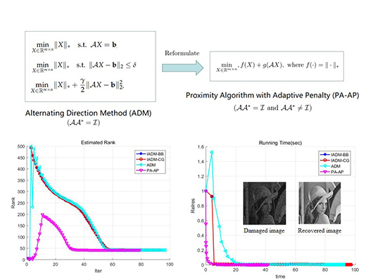
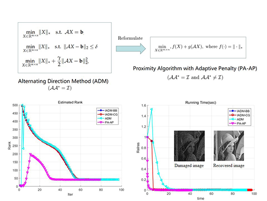
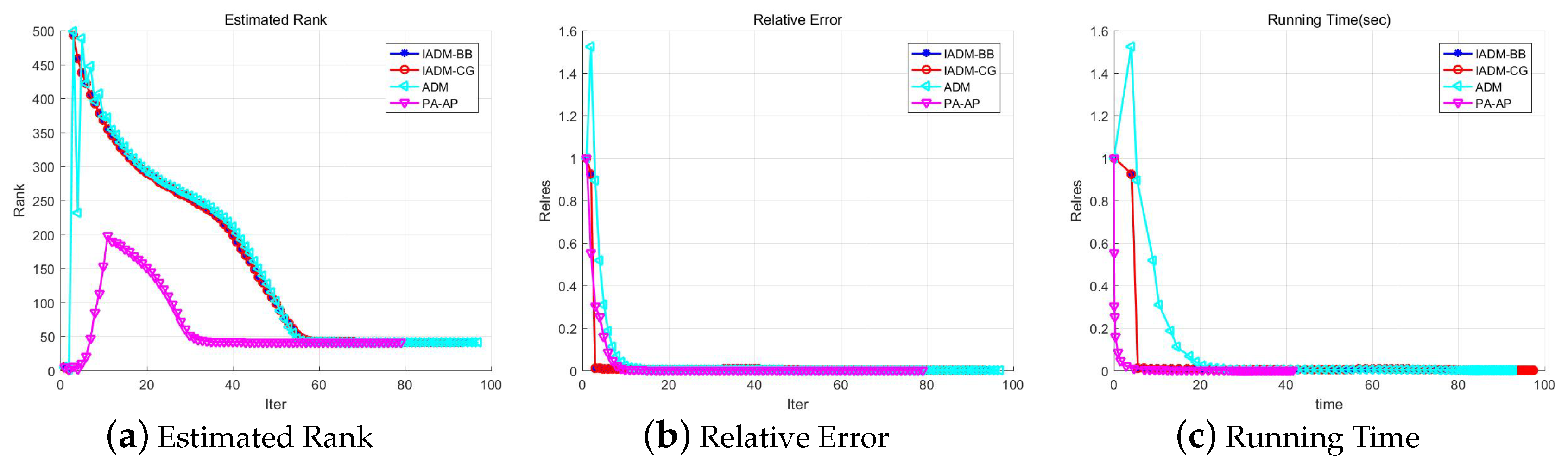
Table 6 shows the cost time, relative error and PSNR of recovery image by different methods. From Table 6, we can note that the PA-AP method is able to obtain higher PSNR as $sr$ increases. Moreover, the running time of PA-AP is always much less than the other methods with different settings. Figure 2 shows the executing process of the different methods. From Figure 2, it is clear that our method can estimate the rank exactly after 30 iterations, and runs much less time before termination than other methods.

Table 6. Comparisons of PA-AP, ADM, IADM-CG and IADM-BB for low-rank image recovery.

Name	sr	PA-AP			ADM			IADM-CG			IADM-BB
		Time	RelErr	PSNR	Time	RelErr	PSNR	Time	RelErr	PSNR	Time	RelErr	PSNR
Lena	0.2	58.66	1.730 × 10−4	26.17	127.86	1.751 × 10−4	26.61	148.71	1.625 × 10−4	26.78	161.59	1.633 × 10−4	26.78
	0.4	46.09	3.984 × 10−5	84.67	94.65	4.578 × 10−5	85.52	94.86	1.191 × 10−4	76.06	110.74	1.244 × 10−4	75.58
	0.6	7.52	2.071 × 10−5	93.42	55.92	2.717 × 10−5	92.60	54.78	8.376 × 10−5	81.65	65.75	9.504 × 10−5	80.40
	0.8	3.41	1.025 × 10−5	101.59	37.32	1.771 × 10−5	99.04	33.46	4.374 × 10−5	89.62	39.09	6.070 × 10−5	86.65
Pirate	0.2	54.23	1.561 × 10−4	26.03	121.73	1.745 × 10−4	26.25	140.40	1.643 × 10−4	26.41	154.24	1.651 × 10−4	26.41
	0.4	38.58	3.961 × 10−5	85.42	92.33	4.905 × 10−5	86.24	94.57	1.140 × 10−4	76.98	112.77	8.735 × 10−5	79.81
	0.6	8.15	1.313 × 10−5	97.97	53.13	2.839 × 10−5	92.92	54.81	4.376 × 10−5	86.89	66.42	6.227 × 10−5	84.26
	0.8	3.45	8.451 × 10−6	104.65	33.83	1.967 × 10−5	99.05	29.41	6.704 × 10−5	91.70	36.86	1.001 × 10−5	88.64
Cameraman	0.2	50.51	1.717 × 10−4	24.10	124.54	1.965 × 10−4	24.32	145.18	2.159 × 10−4	24.43	159.92	2.167 × 10−4	24.43
	0.4	46.81	5.290 × 10−5	80.18	102.31	5.570 × 10−5	81.30	106.05	1.182 × 10−5	73.72	115.48	1.313 × 10−4	73.00
	0.6	10.03	2.389 × 10−5	90.92	59.87	3.090 × 10−5	90.36	58.43	6.099 × 10−5	83.07	71.95	5.343 × 10−5	84.40
	0.8	4.18	1.613 × 10−5	96.46	37.86	2.036 × 10−5	96.03	35.31	3.360 × 10−5	90.22	45.53	2.106 × 10−5	93.04

Figure 2. Convergence behavior of the four methods ($Lena,sr=0.4,{\epsilon }_2={10}^{-5}$). The first subfigure is the estimated rank; the second is the relative error to the original matrix; and the last is the running time.

5. Conclusions and Future Work

In this paper, a unified model and algorithm for the matrix nuclear norm minimization problem are proposed. In each iteration, the proposed algorithm mainly includes computing matrix singular value decompositions and solving proximity operators of two convex functions. In addition, the convergence of the algorithm is also proved. A large number of experimental results and numerical comparisons show that the algorithm is superior to IADM-BB, IADM-CG and ADM algorithms.

The problem of tensor completion has been widely studied recently [31]. One of our future works is to extend the proposed PA-AP algorithm to tensor completion.