Abstract
We explore the role of symmetry in the theory of Special Relativity. Using the symmetry of the principle of relativity and eliminating the Galilean transformations, we obtain a universally preserved speed and an invariant metric, without assuming the constancy of the speed of light. We also obtain the spacetime transformations between inertial frames depending on this speed. From experimental evidence, this universally preserved speed is c, the speed of light, and the transformations are the usual Lorentz transformations. The ball of relativistically admissible velocities is a bounded symmetric domain with respect to the group of affine automorphisms. The generators of velocity addition lead to a relativistic dynamics equation. To obtain explicit solutions for the important case of the motion of a charged particle in constant, uniform, and perpendicular electric and magnetic fields, one can take advantage of an additional symmetry—the symmetric velocities. The corresponding bounded domain is symmetric with respect to the conformal maps. This leads to explicit analytic solutions for the motion of the charged particle.
1. Introduction
In this paper, we explore the role of symmetry in deriving Special Relativity () and in solving relativistic dynamics equations. These symmetries include the isotropy of space and the homogeneity of spacetime. We also show that an auspicious choice of axes preserves a symmetry and leads directly to the Lorentz transformations. By using the symmetric velocity, one can reduce the relativistic dynamics equation to an analytic equation in one complex variable. This leads to explicit solutions.
Albert Einstein developed from two postulates. The first is the “Principle of Relativity,” which states that the laws of physics are the same in all inertial frames of reference. The second postulate states that the speed of light in a vacuum is the same for all observers, regardless of the motion of the light source or the observer. In the approach here, on the other hand, using the above-mentioned symmetries, we derive the Lorentz transformations and the Minkowski metric using only the Principle of Relativity, without assuming the constancy of the speed of light. Instead, in the spirit of Noether’s Theorem, we use the symmetry following from the Principle of Relativity and obtain both a universal speed and a metric, which is conserved in all inertial frames. From the inception of relativity, there were derivations of that did not use the second postulate. The first was by Ignatowsky [1] in 1910. Many other derivations followed; see [2] for a full list of references. Nevertheless, the approach here, based on symmetry, is new.
The plan of the paper is as follows. In Section 2, we give an explicit and quantitative definition of an inertial frame and show that the spacetime transformations between inertial frames are affine. In Section 3, we show that there are only two possibilities for these transformations. The first possibility is the Galilean transformations. The second possibility is the Lorentz transformations. Actually, at this point, the transformations are defined up to a parameter, which a priori depends on the relative velocity between the frames. Nevertheless, after we derive Einstein velocity addition in Section 4, we show that this parameter is independent of the relative velocity. Moreover, this parameter represents the unique speed which is invariant among all inertial frames. The experimental evidence implies that this parameter is c, the speed of light in vacuum. In Section 5, we show that the ball of relativistically admissible velocities is a bounded symmetric domain with respect to the affine automorphisms. We interpret the generators of these automorphisms as forces and use them to derive a relativistic dynamics equation.
An application of relativity theory is solving the dynamics equation for the motion of a charged particle in a constant, uniform electromagnetic field. The dynamics equation derived in Section 5 may be readily solved if , or ( and parallel). The case in which and are perpendicular is harder. In fact, the first explicit lab frame solutions for the case were finally found by Takeuchi [3] in 2002. The approach here relies on an additional symmetry. By changing the dynamic variable from the velocity to the symmetric velocity, the dynamics equation becomes analytic in one complex variable. This leads to analytic solutions in all cases.
We discuss the symmetric velocity and symmetric velocity addition in Section 6. In the following section, we introduce a complexification of the plane of motion and derive the corresponding symmetric velocity addition formula. This leads to a dynamics equation which is analytic in one complex variable.
2. Inertial Frames
We follow Brillouin [4] and consider a frame of reference to be a “heavy laboratory, built on a rigid body of tremendous mass, as compared to the masses in motion”. We introduce 3D spatial coordinates and have a standard clock to measure the spacetime coordinates of events. Our frame of reference is equipped with two devices: an accelerometer and a gyroscope. The accelerometer measures the linear acceleration of our frame, and the gyroscope measures its rotational acceleration.
The next step is defining the concept of “inertial frame”. If, at every rest point of our frame, both the accelerometer and the gyroscope measure zero acceleration, then our frame is an inertial frame. Newton’s First Law states that in an inertial frame, an object moves with constant velocity unless acted upon by a force. This means that a freely moving object has uniform motion. The geometric representation of an object in uniform motion is a straight line in spacetime, for some constant velocity, v. Note that one must consider trajectories in 4D spacetime, not just in space alone. Knowing that an object moves along a straight line in space tells one nothing about whether the object is accelerating.
Consider now an object moving freely in an inertial frame. By the Principle of Relativity, this object’s motion is free in every inertial frame. By the above, the worldline of this object is a straight line in every inertial frame. This means that the spacetime transformations between inertial frames are “affine”. We derive these transformations in the next section.
We mention in passing that, practically speaking, there are no inertial frames, because the massive object to which our frame is attached introduces gravitational forces within the system. Moreover, even in a free-falling frame, where gravitational forces are not felt, there are tidal forces. Therefore, the accelerometer will not measure zero everywhere within the system. Nevertheless, in certain cases, the deviation from inertiality will be small. Examples of such “approximate” inertial frames include a space probe drifting through empty space far away from any massive objects, a satellite orbiting the Earth with the propulsion turned off, a cannonball after being shot from a cannon, an object in a drop tower, and Einstein’s elevator falling towards the Earth. In such a frame, Newton’s First Law holds approximately. An observer in such a frame experiences near weightlessness. In fact, aircraft in free fall are used to train astronauts for the weightless experience. The weightlessness is not perfect, however, because of tidal forces.
From this point on, we work with (true) inertial frames. The next step is to derive the spacetime transformations between them.
3. The Lorentz Transformations
In this section, we derive the Lorentz transformation L between two inertial frames K and , without assuming the constancy of the speed of light. Instead, we use a clever choice of axes, which makes L a symmetry. We obtain, as a consequence, that there is a preserved speed between K and . In the next section, we will show that this speed is independent of the relative velocity between K and . From experimental evidence, we conclude that this speed is c, the speed of light in vacuum.
The Lorentz transformation, L, maps the coordinates of an event in to the event’s coordinates in K. We assume, without loss of generality, that
- the x and axes are antiparallel, whereas the y and axes, as well as the z and axes, are parallel;
- the velocity of in K is a constant in the positive x direction ( is classical, not relativistic); and
- the origins O and correspond at time .
See Figure 1. We use reversed axes to preserve the symmetry between the two frames. In this way, the velocity of K in is also , the same as the velocity of in K. Note that when the x and axes are parallel, the frames K and are said to be in standard configuration. However, in standard configuration, the velocity of K in is . This breaks the symmetry.
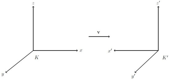
Figure 1.
Two inertial frames with axes antiparallel
One may object that the reversal induces a change of orientation. And even though R is a symmetry, that is, , one may object that it is not a continuous symmetry. Our answer is that continuity will be restored after we determine the transformation , by applying on L.
It follows immediately from condition 2 above that L leaves the y and z coordinates unchanged. Thus, , and we reduce the problem to two dimensions and consider L as a function from to K, with . Now, we invoke the Principle of Relativity, which states that all inertial frames are equivalent. This implies that the spacetime transformations between two inertial frames can depend only on the relative velocity between them. As the velocity of in K is numerically equal to the velocity of K in , the inverse transformation is the same as . In other words,
This means that L is a symmetry. Moreover, as L is affine, condition 3 implies that L is linear.
An independent argument for the linearity of L uses the homogeneity of spacetime (a symmetry) and appears in [5]. First, split L into two functions,
Taking differentials, we have
As spacetime has the same properties everywhere and everywhen, the coefficients cannot depend on t or x. Therefore, F and G are affine functions of and . This, together with condition 3, implies that L is a linear map.
As L is linear, we may represent it in matrix form as
We assume that the time t in K and the time in flow in the same direction. In other words, if t increases, so does . This implies that
Moreover, the velocity of in K is , so
- (I)
- (II)
- (III)
- (IV)
From (I),we get . Let . Then, , or
where we took the positive square root in light of Equation (5).
As , (III) and Equation (5) imply that . Thus,
If , then and . Re-reversing the axis (), we obtain the Galilean transformations:
For the case , we invoke the Principle of Relativity. As the laws of physics are the same in all inertial frames, we look for invariant quantities, quantities which the Lorentz transformations preserve. We search for an invariant metric of the form
where is a positive scalar with dimensions of velocity. Note that may depend on the relative velocity v between K and . By the isotropy of space (a symmetry), the coefficients of , and must be the same, and the homogeneity of spacetime (a symmetry), neither these coefficients nor the coefficient of can depend on any of . Cross-terms like do not appear because such a metric is not invariant under rotations (another symmetry). (One might have thought to define , but this metric leads to physically unreasonable results.)
As we want , we have
or
Thus,
- (1)
- (2)
- (3)
- .
Now , Equation (5) and (1) imply that
Substituting this value for a into (2) yields
It is easy to check that these values for a and satisfy (3). Therefore, there exists an invariant metric of the form Equation (10). Thus, from Equations (8) and (12), the matrix L of the transformation from to K is
Re-reversing the axis (), we obtain the Lorentz transformation :
where .
We would like to show that the scalar is independent of v, but for this, we need velocity addition.
4. Velocity Addition and a Universally Preserved Speed
Einstein velocity addition is actually a composition of velocities and is defined in the following way. Let K and be two inertial frames, where has velocity in K. Suppose an object has velocity in . Then, the velocity of the object in K is denoted by .
To derive a formula for , we take K and in standard configuration, so that . Consider an object with velocity in . Without loss of generality, the object passes through the origin of at time . Therefore, the worldline of the object in is .
Using the Lorentz transformation Equation (14), we have
where and . Thus, the velocity of the object in K is
implying that
For arbitrary and , decompose as , where is the projection of onto and . Then, Equation (16) generalizes to
where is the usual scalar product on . If and are parallel, then
Equations (17) and (18) show that velocity addition is commutative only for parallel velocities. The following two properties will also prove useful.
- (V1)
- (V2)
- If and are parallel, then .
Next, we show that the scalar is independent of v. We assume only a continuity condition, namely, that and can be made arbitrarily close for close enough v and w. Let K and be in standard configuration, where v is the relative velocity of in K. Suppose in K the interval , that is,
so . As the Lorentz transformation preserves the interval, we have , so in , . Note that is the unique speed, which is invariant between K and .
Consider now a third inertial frame , which is in standard configuration with and has relative velocity v in . Repeating the above argument, we see that the speed is invariant between K and . However, the velocity of in K is , implying that the speed is also invariant between K and . By uniqueness, .
Introduce the following notation. For each , define
Note that parentheses are not necessary by (V2). Similarly, we say that iff . In this notation, we have just shown that , or, equivalently, . It is easy to show by induction on n that for all n, and so for all n.
It remains to show only that for arbitrary (parallel) velocities v and w. There are positive integers m and n, such that and are arbitrarily close. By the continuity condition, and are arbitrarily close. Therefore, and are arbitrarily close. We conclude that .
Several experiments at end of nineteenth century, including [6], showed that the speed of light is the same in all inertial systems. Therefore, , the speed of light in vacuum, and the Lorentz transformation is
where .
Note that velocity addition Equation (17) maps a subluminal (less than c) velocity to a subluminal velocity. Subluminal velocities are appropriate for massive particles. There are also particles, such as photons, with speed c in every inertial frame. Our theory does not preclude the existence of superluminal velocities, nor does it predict them.
At this point, we introduce the dimensionless velocity and rename it . Thus, a velocity is subluminal if . This amounts to measuring time in light seconds (or light years).
5. The Velocity Ball as a Bounded Symmetric Domain
The velocity ball is defined as the set of all subluminal velocities
We study the symmetries on that follow from the Principle of Relativity.
A domain D in a real or complex Banach space is called symmetric with respect to a group G of automorphisms of D if for every , there is an automorphism , such that g is a symmetry () and g fixes only the point a.
Clearly, is a bounded domain. We show here that is symmetric with respect to the group of affine automorphisms of . An automorphism is affine if it maps lines to lines.There is an obvious affine symmetry, namely, , which fixes only 0. By shifting this map, we can get an affine symmetry about any given point.
The symmetries we require are constructed from the velocity addition, so let us first understand how velocity addition acts on . For each , define the map by
By the velocity addition Equation (17), the image of a disc in perpendicular to is also a disc in , moved in the direction of , and uniformly scaled in the component, see Figure 2.
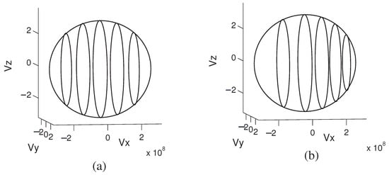
Figure 2.
(a) Five uniformly spread discs , obtained by intersecting the three-dimensional velocity ball of radius 1 with planes at . (b) The images of the five discs under the action of , with .
We show now that for each , the map , defined by Equation (22), is an affine automorphism of . Clearly, is a bijection. Velocities that are different in K are different in , and every velocity in has a corresponding velocity in K. Moreover, the inverse of is
The proof of affinity is via the projective geometry of the velocity ball . We identify each as the point of intersection of the worldline of an object with velocity and the plane . A segment T in is the intersection of with a plane, Q, through the spacetime origin, O, of K. The Lorentz transformation maps Q to a plane, , through the spacetime origin of . The image of T under is the intersection of with and is therefore a segment. This shows that is an affine map.
Fix , and let . Note that : the symmetric velocity corresponding to . Define by
We claim that is an affine automorphism of and a symmetry fixing only the symmetric velocity .
The map is a composition of affine automorphisms of , and is therefore an affine automorphism of . The map is a symmetry because, using Equation (24) and (V1) and (V2),
The map fixes , as
The map fixes only . Suppose . From the definition Equation (17) of velocity addition, it follows that . Then, as fixes and using (V2), we have
so . This completes the proof that is a bounded symmetric domain with respect to the group of affine automorphisms of .
Next, we characterize the elements of . Let be any affine automorphism of . Set and . Then, U is an affine map that maps and is thus a linear map which can be represented by a matrix, which we also call U. As U maps onto itself, it is an isometry and U is an orthogonal matrix. As , the group of all affine automorphisms is given by
where is the group of orthogonal transformations of . The group is a six-dimensional real Lie group. Three dimensions are needed to determine the boost vector , and three dimensions determine the orthogonal matrix . This gives a representation of the Lorentz group by affine maps of .
It is well known that a force generates an acceleration, which is a change in velocity. There are two types of forces. The first type generates a change in the magnitude of the velocity and can be modeled by a velocity boost. An example is the force exerted by an electrostatic field on a charged particle. The second type of force generates a change in the direction of the velocity and can be modeled by a rotation. Such a force generates an acceleration in a direction perpendicular to the velocity of the object. An example is the force exerted by a magnetic field on a moving charge.
For example, the generator of the boost is given by
Using the triple product , defined by
the above generator can be written as
In [7], the first author calculates the elements of the Lie algebra and shows that the generators of boosts act on like an electric field, and the generators of rotations act on like a magnetic field. The classical equation of motion
for a particle of charge, q, and mass, m, in an electromagnetic field , is then shown to be equivalent to
where is the rest mass of the particle, and is the proper time of the particle. The relationship between t and is given by .
For constant, uniform fields and , Equation (29) can be solved in a straightforward manner in the three cases , and ( and are parallel). See [7] for details. The case in which and are perpendicular presents more difficulties. The standard approach (see, for example, ref. [8,9]) solves Equation (28) in the well-known drift frame. In the case , it is then straightforward to transform the solution back to the lab frame. None of the standard texts, however, obtain explicit solutions in the lab frame for the case . The first explicit lab frame solutions were found by Takeuchi [3] in 2002.
The case is greatly simplified if we make a change of dynamic variable and use the symmetric velocity instead of the usual velocity. We take this up in the next section.
6. The Symmetric Velocity Ball as a Bounded Symmetric Domain
The procedure of the previous section may be applied to the ball of symmetric velocities. One defines symmetric velocity addition and shows that the action induced on the ball by a “boost” is a conformal map. Indeed, one can show that the symmetric velocity ball is a bounded symmetric domain with respect to the group of conformal automorphisms. See Chapter 2 of [7] for the details of this and the next two sections.
As in the previous section, the relativistic dynamics equation for symmetric velocities can be written in terms of generators—this time, the generators of conformal maps. Moreover, in the historically troublesome case , the dynamics equation becomes analytic in one complex variable. This leads to explicit analytic solutions.
In this section and the next, we develop the tools necessary to work with the symmetric velocity.
As defined just prior to Equation (24), the symmetric velocity corresponding to the velocity is the unique velocity , such that . The relationship between a symmetric velocity , and its corresponding velocity is given by
The symmetric velocity ball is the set of all relativistically admissible symmetric velocities:
Addition (composition) of symmetric velocities is defined using Einstein velocity addition and the map . Let and be symmetric velocities. Then,
A straightforward albeit tedious calculation leads to the following symmetric velocity addition formula,
A 4D version of Equation (33) can be found in [10].
As in Equation (22), we define, for each , the map by
In [7], it is shown that is a conformal map and that is a bounded symmetric domain with respect to the group of conformal automorphisms of . Moreover,
The group is a six-dimensional real Lie group. Three dimensions are needed to determine the boost vector , and three dimensions determine the orthogonal matrix . This gives a representation of the Lorentz group by conformal maps of .
Similar to Equation (27), the generator of the boost is given by
where the spin triple product [11] is defined by
Equation (28) can then be written as
As in Equation (29), is the proper time of the particle. Once one obtains an explicit solution for , the time t can be calculated using
The coefficient of is so as to obtain the correct commutation relations.
Under certain initial conditions, the solutions to Equation (38) will be planar. We will see next how symmetric velocity addition acts on the complexified plane of motion.
7. Symmetric Velocity Addition on a Complex Plane
Equation (33) shows that is a linear combination of and , and therefore belongs to the plane generated by and . We introduce a complex structure on in such a way that the disk is homeomorphic to the unit disc . Denote by a the complex number corresponding to the vector and by w the complex number corresponding to the vector . We make use of the familiar relationships
where the dot product is the usual one on , and the bar denotes complex conjugation. Substituting these into Equation (33), we get
which is the well-known complex analytic Möbius transformation of the complex unit disk. Thus, symmetric velocity addition is a generalization of the Möbius addition of complex numbers.
In Figure 3, the lower circle in the figure is the unit disc of the complex plane, a two-dimensional section of . The upper circle is the image of the lower circle under the transformation , for . Each circle is enhanced with a grid to highlight the effect of this transformation. Notice how a typical square of the lower grid is deformed and changes in size under the transformation.
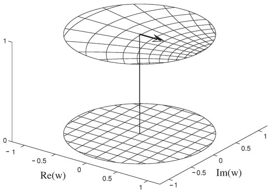
Figure 3.
Symmetric velocity addition for .
8. Explicit Analytic Solutions When
We will use a complexified version of Equation (38) to find explicit analytic solutions for motion in constant, uniform fields , where and are perpendicular. We assume that the initial velocity is perpendicular to . In this case, the motion remains in the plane , which is perpendicular to . This follows from the fact that the right side of Equation (38) is in at and belongs to this plane.
We will complexify the plane so that the vector lies on the positive part of the imaginary axis. We associate to any symmetric velocity a complex vector , with real . The vector will be represented by the complex number . In this representation, the vector , which is in , is equal to . Using Equation (40), the term is represented by the complex number
Equation (38) becomes
For notational convenience, we introduce the constants
which allows us to rewrite Equation (44) as
which is a first-order, complex analytic, separable differential equation. By a well-known theorem from differential equations, this equation has an analytic solution, which is unique for each initial condition, . Equation (46) may be solved straightforwardly for in all three cases, , , and . The velocity may then be found using Equation (30) and the position via integration.
When , the symmetric velocity traces out a circular trajectory. When , the trajectories are arcs of circles and . The symmetric velocities for are also arcs of circles, but with finite terminal velocity. For more details and examples, see [12].
9. Discussion
We have taken advantage of several symmetries to develop the Special Theory of Relativity without assuming the constancy of the speed of light. These symmetries include the principle of relativity, the isotropy of space, and the homogeneity of spacetime. We also made an auspicious choice of axes to preserve a symmetry between inertial frames. Eliminating the Galilean transformations, we obtained a universally preserved speed and an invariant metric. The ensuing spacetime transformations between inertial frames depend on this speed. From experimental evidence, this universally preserved speed is c, the speed of light, and the transformations become the usual Lorentz transformations Equation (14).
The velocity ball is a bounded symmetric domain with respect to the affine automorphisms induced by velocity addition. We represent an electromagnetic field by the generators of these automorphisms and derive a dynamics Equation (29). This equation can be solved explicitly in certain cases.
The other cases require the symmetric velocity ball, which is a bounded symmetric domain with respect to the conformal automorphisms induced by symmetric velocity addition. There is a canonical representation of the Lorentz group into the Lie algebra of conformal generators. The dynamics Equation (38) is built from these generators, and under the right initial conditions, the dynamics equation becomes analytic in one complex variable. This leads to explicit solutions.
It should be noted that the dynamics Equation (29) is Lorentz covariant with respect to affine maps. Likewise, Equation (38) is Lorentz covariant with respect to conformal maps. One can obtain Lorentz covariance with respect to linear maps by using a 4D representation. In fact, Equation (28) is canonically embedded in the fully Lorentz covariant dynamics equation
where is the four-velocity, and is a rank 2 antisymmetric tensor with units of acceleration. The components of A, in general, are functions of spacetime. For constant A, the explicit solutions of Equation (47) are divided into four Lorentz-invariant classes: null, linear, rotational, and general. For null acceleration, the worldline is cubic in the time. Linear acceleration covariantly extends one-dimensional hyperbolic motion, whereas rotational acceleration covariantly extends pure rotational motion. See [13] for details.
A motion is uniformly accelerated if it has constant motion in the instantaneously comoving inertial frame. In [14], Equation (47) is extended a system of differential equations which define this so-called generalized Fermi–Walker frame. It is shown in [15], that, in flat spacetime, when A is constant, a motion is uniformly accelerated if and only if it satisfies Equation (47). Thus, Equation (47) provides a complete and covariant description of uniformly accelerated motion.
We note that the approach of the authors of [13,14,15] is equivalent to that of B. Mashhoon [16,17]. Mashhoon works on a manifold, and so his approach is frame-independent, whereas our definition is with respect to a particular inertial frame. On the other hand, Mashhoon’s system of differential equations is coupled, and therefore harder to solve.
Reference [15] also contains velocity and acceleration transformations from a uniformly accelerated frame to an inertial frame, as well as the time dilation between clocks in a uniformly accelerated frame. The power series expansion of our time dilation formula contains all of the usual terms, but also an additional term that had only been obtained previously in Schwarzschild spacetime. We applied these results to the case of an accelerated charge and obtained the Lorentz–Abraham–Dirac equation
where the triple product Equation (26) has been extended to 4D using the Minkowski inner product.
The theory extends to curved spacetimes ([18]). Given an arbitrary curved spacetime, there is a system of nonlinear first-order differential equations that extends the geodesic equation, and whose solutions are precisely the uniformly accelerated motions in the given spacetime. This improved a result of [19], whose corresponding equation models only hyperbolic motion. We consider the particular case of radial motion in Schwarzschild spacetime and show that in this situation, there are no bounded orbits.
The theory of Special Relativity developed here is local and assumes that physical phenomena can be reduced to pointlike coincidences. However, many phenomena are nonlocal. The measurement of the electromagnetic field, for example, is not instantaneous but usually averaged over a spacetime domain [20,21]. Similarly, the Huygens principle implies that wave phenomena are, in general, not local. The “Hypothesis of Locality,” used to obtain the transformations of [14,15], states that an accelerated observer is at each instant physically equivalent to a hypothetical inertial observer that is otherwise identical and instantaneously comoving with the accelerated observer. As shown in [22], this hypothesis is inconsistent with quantum theory. Thus, it is necessary to develop a nonlocal theory of relativity. One possible approach is to take advantage of the properties of bounded symmetric domains, using the techniques found in [23], for example. We hope to develop a nonlocal theory in the future.
Author Contributions
Conceptualization, Y.F. and T.S.; methodology, Y.F. and T.S.; writing—original draft preparation, Y.F. and T.S.; writing—review and editing, Y.F. and T.S.
Funding
This research received no external funding.
Acknowledgments
The authors would like to thank the four reviewers for helpful comments and suggestions.
Conflicts of Interest
The authors declare no conflicts of interest.
References
- Von Ignatowsky, W.A. Einige allgemeine Bemerkungen zum Relativitätsprinzip. Verh. Deutsch. Phys. Ges. 1910, 12, 788–796. [Google Scholar]
- Baccetti, V.; Tate, K.; Visser, M. Inertial frames without the relativity principle. J. High Energy Phys. 2012, 119. [Google Scholar] [CrossRef]
- Takeuchi, S. Relativistic E×B acceleration. Phys. Rev. E 2002, 66. [Google Scholar] [CrossRef] [PubMed]
- Brillouin, L. Relativity Reexamined; Academic Press: New York, NY, USA, 1970. [Google Scholar]
- Lévy-Leblond, J. One more derivation of the Lorentz transformation. Am. J. Phys. 1976, 44, 271–277. [Google Scholar] [CrossRef]
- Michelson, A.; Morley, E. On the Relative Motion of the Earth and the Luminiferous Ether. Am. J. Sci. 1887, 34, 333–345. [Google Scholar] [CrossRef]
- Friedman, Y. Physical Applications of Homogeneous Balls. In Progress in Mathematical Physics; Birkhauser: Boston, MA, USA, 2004; Volume 40. [Google Scholar]
- Jackson, J. Classical Electrodynamics, 3rd ed.; Wiley: New York, NY, USA, 1999; Volume 586–588, pp. 617–618. [Google Scholar]
- Landau, L.; Lifshitz, E. The Classical Theory of Fields, 4th ed.; Pergamon Press: Oxford, UK, 1975; pp. 43–65. [Google Scholar]
- Mashhoon, B. Conformal Symmetry, Accelerated Observers, and Nonlocality. Symmetry 2019, 11, 978. [Google Scholar] [CrossRef]
- Dang, T.; Friedman, Y. Classification of JBW*-triple factors and applications. Math. Scand. 1987, 61, 292–330. [Google Scholar] [CrossRef]
- Friedman, Y.; Semon, M. Relativistic acceleration of charged particles in uniform and mutually perpendicular electric and magnetic fields as viewed in the laboratory frame. Phys. Rev. E 2005, 72, 026603. [Google Scholar] [CrossRef] [PubMed]
- Friedman, Y.; Scarr, T. Making the Relativistic Dynamics Equation Covariant: Explicit Solutions for Constant Force. Phys. Scr. 2012, 86, 065008. [Google Scholar] [CrossRef]
- Friedman, Y.; Scarr, T. Spacetime Transformations from a Uniformly Accelerated System. Phys. Scr. 2013, 87, 055004. [Google Scholar] [CrossRef]
- Friedman, Y.; Scarr, T. Uniform Acceleration in General Relativity. Gen. Relativ. Gravit. 2015, 47, 121. [Google Scholar] [CrossRef]
- Mashhoon, B. Limitations of spacetime measurements. Phys. Lett. A 1990, 143, 176–182. [Google Scholar] [CrossRef]
- Mashhoon, B. The hypothesis of locality in relativistic physics. Phys. Lett. A 1990, 145, 147–153. [Google Scholar] [CrossRef]
- Friedman, Y.; Scarr, T. Solutions for Uniform Acceleration in General Relativity. Gen. Relativ. Gravit. 2016, 48, 65. [Google Scholar]
- De la Fuente, D.; Romero, A. Uniformly accelerated motion in General Relativity: Completeness of inextensible trajectories. Gen. Relativ. Gravit. 2015, 47, 33. [Google Scholar] [CrossRef]
- Bohr, N.; Rosenfeld, L. Zur Frage der Messbarkeit der elektromagnetischen Feldgrössen. R. Dan. Acad. Sci. Lett. J. Math. Phys. 1933, 12, 8. [Google Scholar]
- Bohr, N.; Rosenfeld, L. Field and charge measurements in quantum electrodynamics. Phys. Rev. 1950, 78, 794–798. [Google Scholar] [CrossRef]
- Mashhoon, B. Nonlocal Special Relativity. Ann. Phys. 2008, 17, 705–727. [Google Scholar] [CrossRef]
- Faraut, J.; Kaneyuki, S.; Korányi, A.; Lu, Q.; Roos, G. Analysis and Geometry on Complex Homogeneous Domains; Birkhauser: Boston, MA, USA, 2000. [Google Scholar]
© 2019 by the authors. Licensee MDPI, Basel, Switzerland. This article is an open access article distributed under the terms and conditions of the Creative Commons Attribution (CC BY) license (http://creativecommons.org/licenses/by/4.0/).