Comparative Evaluation of Algorithms for Spatial Interpolation of Atmospheric State Parameters Based on a Dynamic Stochastic Model Taking into Account the Vertical Variation of a Meteorological Field

Abstract

The paper presents a comparative analysis of two algorithms for the spatial interpolation of meteorological fields. Both algorithms are based on a four-dimensional low-order parametric dynamic stochastic model, taking into account the vertical variation of a meteorological field. The algorithms are characterized by different representations of the forecast model in state and observation space equations for the Kalman filter. The authors studied the accuracy of the spatial interpolation of temperature and wind fields for the developed algorithms. The results of the study are presented in this paper. Numerical simulation was conducted using long-term upper-air observations obtained for a typical mesometeorological range. The results of the study demonstrate that the accuracy of interpolation for the two considered algorithms is comparable.

1. Introduction

The state of the atmosphere at a given time (or for a given period) over any place or region of the globe is characterized by a combination of meteorological variables, such as pressure, temperature and humidity, wind speed and direction, cloud cover, precipitation, as well as by specific phenomena such as fog, thunderstorms, snowstorms, etc. For objective reasons, it is impossible to obtain reliable measurement data from every point on the globe. This is due to the fact that the existing network of weather and upper-air stations is unevenly distributed across the planet and almost not available in some areas. For example, in Eurasia, high-density networks of measuring stations can be found in the industrially developed countries of Central Europe. Networks in underdeveloped regions of Central Asia are rare or completely absent. The current remote space-based facilities cannot yet provide measurements with the necessary accuracy and frequency. Therefore, the applied meteorology focuses on diagnosing and predicting the state of the atmosphere over the areas poorly covered by meteorological observations and, accordingly, on developing solutions to this problem. This is especially important for mesoscale, i.e., for the areas with linear dimensions of 20–500 km and a height of the upper boundary up to 10 km. This is because the vast majority of applied problems related to air basin monitoring are solved at a local level, within large cities and large industrial centers. In particular, modeling and predicting the spatial distribution of industrial pollutants within small (up to 100–500 km) distances from emission sources plays an important role in the environmental protection system. Other important problems include the assessment and forecast of weather conditions in the areas affected by industrial or natural disasters. Meteorological support is also necessary for applied problems of radiophysics, radiolocation, radio navigation, and telecommunications, as well as for assessing the attenuation and transformation of electromagnetic radiation during atmospheric propagation. They are also needed to study environmental effects on the performance of optical space systems, to interpret multispectral satellite measurements and laser location data on atmospheric parameters.

Areas in which a network of weather stations is rare or absent face a problem regarding the spatial restoration of meteorological fields using data from stations located in adjacent areas. Previously, problems of spatial extrapolation have traditionally been solved using a fact-based analysis of meteorological fields based on methods of polynomial [1,2] and spline [3] approximation, as well as optimal interpolation (extrapolation) [4,5,6,7,8]. Currently, the meteorological data assimilation procedure is used to solve these problems [9,10,11,12,13]. To date, a number of methods have been developed with different initial forecast models and algorithms for the numerical processing of measurement data. These methods combine forecast and fact-based analysis of meteorological fields, and simultaneously take into account both measurements themselves and the results of spatial extrapolation based on a selected mathematical model. The weather forecast over the area covered by measurements is an extrapolation of current weather conditions in time [4,5]. Extrapolation in space is used to extend meteorological fields to areas not covered by observations (extrapolation in a horizontal plane) [7], as well as to restore fields at high altitudes according to data for underlying levels (vertical extrapolation) [14,15].

Methods for the interpolation and extrapolation of meteorological fields can be divided into dynamic, statistical, dynamic stochastic, and formal. The dynamic methods are methods based on equations of atmospheric hydrodynamics and thermodynamics. For example, the numerical forecast (hydrodynamic) methods are based on extrapolating meteorological fields in time and space [8,16,17,18]. The methods that provide, when applied repeatedly, the best results in relation to a particular statistical variable are called statistical [4,17]. These methods are based on the patterns identified by the statistical processing of bulk meteorological data.

The ‘formal’ methods refers to methods based on the assumptions that follow neither from the laws of atmospheric dynamics nor from empirical laws. The synoptic method is the best-known formal method [18]. The formal methods also include the extrapolation of pressure fields, which is based on the assumption that the velocity of wind and pressure systems remains constant during the forecast period. These methods also include the interpolation methods based on the expansion of fields in a certain system of specified functions, which provide satisfactory forecast results in simple situations [4].

The dynamic stochastic methods are implemented within the framework of the optimal estimation theory based on Kalman filtering techniques [7,19,20,21,22]. This approach assumes that the current atmospheric state can be represented by random fields, which are described by a system of dynamic stochastic equations. The forecast models for these methods are defined as a system of first-order stochastic differential equations for the variables to be estimated. In this case, both linear and nonlinear functions can be used for models. Unknown meteorological variables are estimated recursively as current measurement data become available. The development of the dynamic stochastic approach has led to the creation of the methods based on the ensemble Kalman filter (EnKF) [23] and its various modifications [24,25,26,27,28,29]. Currently, this approach is most often used to assimilate meteorological data and extrapolate meteorological fields.

When applying the Kalman filter to data assimilation using complex equations of hydrodynamics, researchers face a number of challenges associated with a high dimension of the forecast error covariance matrix [9,10,16,22,23,24]. Therefore, some authors paid considerable attention to the development of interpolation (extrapolation) algorithms based on the dynamic stochastic approach and low-parameter models. [14,15,19,20,21,22] summarize studies of various methods developed for evaluating and predicting atmospheric state parameters for a mesometeorological scale. Various types of forecast models (low-order parametric dynamic stochastic, polynomial, regression, etc.) were used to synthesize the filtering algorithm.

Our previous studies [14,15] proposed a simplified four-dimensional model that represents the evolution of meteorological variables in time and space for a mesometeorological scale. The dynamic stochastic model considers spatial and temporal changes in meteorological fields as random processes with known correlation properties. The algorithm based on the linear Kalman filter (LKF) is used to estimate (in fact, interpolate) a meteorological variable for a given point in space according to observations from several available weather stations. In order to restore meteorological fields over a limited area (for example, to nodes of a regular grid in three-dimensional space), an ensemble of filters should be used. This approach limits the dimension of state and observation vectors, reduces the dimension of forecast and estimation error covariance matrices, and therefore, simplifies the implementation of the filtering algorithm.

In this paper, we use a low-order parametric dynamic stochastic model with a vertical component based on a four-dimensional differential equation. It should be noted that based on this model, researchers have developed two filtering algorithms that ensure the interpolation of meteorological fields at the mesoscale [14,15]. These algorithms are characterized by different representations of the initial forecast model in state and observation space equations in terms of the Kalman filter.

Thus, the aim of this paper is to consider the structural differences between the two algorithms [14,15], and to assess the effects of these differences on the accuracy of interpolation of meteorological fields.

2. Problem Statement and Features of the Proposed Approach

2.1. General Problem Statement and Description of the Model

Let us briefly state the problem considered earlier in [14,15] in general form. Assume that (s + 1) of spatially separated points with known coordinates (x_i, y_i), where i = 0, …, s, is given in the mesoscale range at the ground level. Regular upper-air measurements of meteorological variables (temperature and orthogonal wind velocity components) were conducted in the vertical profile of the atmosphere above points i = 1, …, s. It should be noted that such measurements are absent for point i = 0 with coordinates (x₀, y₀). The restoration of the meteorological field ξ₀ at point i = 0 implies estimating its values from the measurements obtained at points i = 1, …, s. According to [21,22], the resulting estimate of the field ${\xi }_0$ at the required point (x₀, y₀) is determined as the sum of the random ${\xi }_0^{\prime }$ and regular ${\overline{\xi }}_0$ components:

$${\xi }_0={\xi }_0^{\prime }+{\overline{\xi }}_0.$$

(1)

The average value of the data from three nearby measuring stations calculated for a specific height h is used as a regular field component.

$${\overline{\xi }}_0={\displaystyle \sum _{i=1}^3{q}_i{\xi }_i}/{\displaystyle \sum _{i=1}^3{q}_i},$$

(2)

where ${\xi }_i$ v i, $q_i=1-({\rho }_{i0}/{\displaystyle \sum _{i=1}^3{\rho }_{i0}})$ is the weighting factor, and ${\rho }_{i0}=\sqrt{{{(x}_i{-x}_0)}^2+{{(y}_i{-y}_0)}^2}$ is the distance between the weather station i and the forecast point (i = 0).

To describe the random component ${\xi }_0^{\prime }$, we use a dynamic stochastic model with two equations:

$${\xi }_i^{\prime }(k+1)={\xi }_0^{\prime }(k)(1-\alpha \Delta t)(1-\beta \Delta {\rho }_{i0})(1-\gamma \Delta h)+{\mathsf{\epsilon }}_i(k),$$

(3)

$${\xi }_0^{\prime }(k+1)={\xi }_0^{\prime }(k)(1-\alpha \Delta t)+{\mathsf{\epsilon }}_0(k),$$

(4)

where $\alpha$ and $\beta$ are the coefficients that determine the temporal and spatial relationships among the data of upper-air stations within the mesoscale range; $\gamma$ is the coefficient that determines the inter-level relationship of meteorological fields; k is the discrete time; and $\epsilon$ is the noise of the model that determines the random nature of atmospheric processes.

Equation (3) demonstrates the temporal and spatial relationship between the interpolation point and the measuring stations. Equation (4) describes changes in the field in time directly at the interpolation point. Statistical properties of the atmospheric parameters can be described by correlation functions using the following exponential expressions: $\mu (\tau )=\exp (-\alpha \tau )$ in time, $\mu (\rho )=\exp (-\beta \rho )$ in the horizontal plane, and the correlation function of height $\mu (h)=\exp (-\gamma h)$. Where $\alpha =1/{\tau }_0$, $\beta =1/{\rho }_0$, $\gamma =1/h_0$ are the coefficients that are inversely proportional to the intervals of temporal, spatial, and inter-level correlation, respectively.

As compared to the model [21,22], based on the two-dimensional mesoscale diffusion equation, the proposed model [14,15] includes a new element that is responsible for vertical correlation, as shown in Equation (3). Meteorological variables at the interpolation point (x₀, y₀) are unknown and need to be estimated. The coefficients $\alpha$, $\beta$, and $\gamma$ should be determined in advance during the preliminary analysis of the upper-air data obtained for the selected mesoscale range. This is because the meteorological fields can be considered to be homogeneous and isotropic for time intervals between upper-air observations and within the selected mesoscale range (maximum size 500 × 500 km).

Equations (3) to (4) can be represented as a system of difference first-order equations [30] with the following matrix form:

$$x_{k+1}^t={\mathsf{\psi }}_k{x}_k^t+{\mathsf{\omega }}_k^t,$$

(5)

where $x_k^t$ is the state vector, including unknown variables to be estimated, at time k; ${\mathsf{\psi }}_k$ is the transition matrix for a linear discrete system; ${\mathsf{\omega }}_k^t$ is the state noise vector; and t stands for true values.

The general observation model should be represented by a sum of the true value of the meteorological variable and the observational error at the measurement point i [30]:

$$z_k^o=H_k{x}_k^t+{\epsilon }_k^o,$$

(6)

where $z_k^o$ is the observation vector, including a set of centered measurements obtained at stations at time k; $H_k$ is the observation matrix that determines the functional relationship between state variables and current measurements; ${\epsilon }_k^o$ is the vector of observational errors at time k; and the symbol o stands for observations.

Recall that this paper considers two interpolation algorithms [14,15], in which Equations (3)–(6) is used in different representations. Accordingly, the dimension and content of the matrices ${\mathsf{\psi }}_k$ and $H_k$ for the developed algorithms will be different. In any case, the coefficients $\alpha$, $\beta$, and $\gamma$ are estimated a priori, separately from the filtering algorithm.

2.2. Kalman Filter Structure for the First Variant of the Interpolation Algorithm

In the first case [14], the state vector $x_k^t$ consists of a single element shown in Equation (4), which is the value of the required meteorological variable at the point with the coordinates (x₀, y₀) for a given height level h at time k. Therefore, the transition matrix also consists of a single element:

$${\mathsf{\psi }}_{1,k}=\Vert 1-\alpha \Delta t\Vert .$$

(7)

where ${\mathsf{\psi }}_{1,k}$ is the transition matrix for the first interpolation algorithm [14]; and subscript “1” indicates that the transition matrix is defined specifically for the first algorithm.

In turn, the vector $z_k^o$ consists of centered values of meteorological variables, as shown in Equation (8), where it is represented as elements of the vertical profiles obtained for all observation stations s at synchronous times k:

$$z_k^o={\Vert z_{11}^o(k),z_{10}^o(k),z_{12}^o(k),z_{21}^o(k),z_{20}^o(k),z_{22}^o(k),\dots ,z_{s2}^o(k)\Vert }^{\mathrm{T}}.$$

(8)

The first subscript of each element of the observation vector ($z_{ij}^o$) shows the number of a measuring station (i = 1, …, s), and the second subscript stands for the number of the height level (j = 0, 1, 2). Here, the element of the height profile is defined by three successive levels: below (j = 1); above (j = 2), and at the level of the estimation point (j = 0). The levels are selected on the basis of the applicable height grid. The height difference between the levels is $\Delta h_{10}$ and $\Delta h_{20}$, respectively. According to Equation (8), the dimension of the observation vector $z_k^o$ is equal to (3s × 1).

The comparison of Equations (3) and (8) shows that the elements of the observation matrix in Equation (6) consist of the coefficients $\beta$ and $\gamma$, which represent the horizontal and vertical spatial correlations of meteorological fields:

$$H_{1,k}=\Vert \begin{array}{l}(1- {\gamma }_{10}\Delta h_{10})(1- \beta \Delta {\rho }_{10})\\ (1-\beta \Delta {\rho }_{10})\\ (1- {\gamma }_{20}\Delta h_{20})(1-\beta \Delta {\rho }_{10})\\ (1- {\gamma }_{10}\Delta h_{10})(1-\beta \Delta {\rho }_{20})\\ \dots \\ (1- {\gamma }_{20}\Delta h_{20})(1-\beta \Delta {\rho }_{s0})\end{array}\Vert ,$$

(9)

where ${\gamma }_{10}$ and ${\gamma }_{20}$ are the values that determine the vertical inter-level correlation between the given height levels (1-0) and (2-0), respectively; while $\Delta {\rho }_{s0}$ is the distance between the station s and the interpolation point. Accordingly, the dimension of the matrix $H_{1,k}$ is equal to (3s × 1).

2.3. Kalman Filter Structure for the Second Variant of the Interpolation Algorithm

In the second case [15], the state vector $x_k^t$ consists of n elements and includes the meteorological variables to be estimated:

$$x_k^t=\left|x_1(k), x_2(k), x_3(k), \dots ,x_n(k)\right|=\left|{\xi }_0^{\prime }(k), {\xi }_1^{\prime }(k), {\xi }_2^{\prime }(k), \dots ,{\xi }_{3S}^{\prime }(k)\right|.$$

(10)

The elements of the vector ${\xi }_0^{\prime }$ and ${\xi }_i^{\prime }$ in Equations (3) and (4) determine the values of meteorological variables at different points of the mesoscale range. According to Equations (3), (4) and (10), the transition matrix for the second interpolation algorithm [15] is given by:

$${\mathsf{\psi }}_{2,k}=\Vert \begin{array}{cccc}(1-\alpha \Delta t)& 0& \cdots & 0\\ (1-\alpha \Delta t)(1-\beta \Delta {\rho }_{10})(1-{\gamma }_{10}\Delta h_{10})& 0& \cdots & 0\\ (1-\alpha \Delta t)(1-\beta \Delta {\rho }_{10})& 0& \cdots & 0\\ (1-\alpha \Delta t)(1-\beta \Delta {\rho }_{10})(1-{\gamma }_{20}\Delta h_{20})& 0& \cdots & 0\\ (1-\alpha \Delta t)(1-\beta \Delta {\rho }_{20})(1-{\gamma }_{10}\Delta h_{10})& 0& \cdots & 0\\ \cdots & \cdots & \cdots & \cdots \\ (1-\alpha \Delta t)(1-\beta \Delta {\rho }_{s0})(1-{\gamma }_{20}\Delta h_{20})& 0& \cdots & 0\end{array}\Vert .$$

(11)

According to Equations (8) and (10), the observation matrix for the second interpolation algorithm [15] is given by:

$$H_{2,k}=\Vert \begin{array}{ccccc}0& 1& 0& \dots & 0\\ 0& 0& 1& \dots & 0\\ 0& 0& 0& \dots & 0\\ \dots & \dots & \dots & \dots & \dots \\ 0& 0& 0& \dots & 1\end{array}\Vert .$$

(12)

The dimension of the observation matrix $H_{2,k}$ is equal to (3 s) × (3 s + 1).

2.4. General Matrix Expressions for the Synthesized Algorithms

To develop the interpolation algorithms, we used the classical matrix equations of the linear Kalman filter [14,15,30], which provides an estimate of all the elements of the state vector shown in Equations (5) and (10) with a minimum value of the root mean square (RMS) error. Matrices (7), (9) and (11), (12) completely determine the filter (LKF) structure, which makes it possible to estimate the meteorological variable at a point with coordinates (x₀, y₀) at height h.

The basic matrix equation for the Kalman filter is given by [30]:

$$x_k^a=x_k^f+K_k(z_k^o-H_k{x}_k^f),$$

(13)

where $x_k^a$ is the estimate (analysis) of the state vector at time k; $x_k^f$ are the predicted values for the state vector at time k; and $K_k$ is the weighting matrix. The matrix $K_k$ for the linear Kalman filter is calculated using the following recurrence equations [30]:

$$K_k=P_k^f{H}_k^{\mathrm{T}}{(H_k{P}_k^f{H}_k^{\mathrm{T}}+R_k)}^{-1}$$

(14)

$$P_k^f={\mathsf{\psi }}_k{P}_{k-1}^a{\mathsf{\psi }}_k^{\mathrm{T}}+Q_{k-1},$$

(15)

$$P_k^a=(I-K_k{H}_k)P_k^f,$$

(16)

where $P_k^a=<(x_k^a-x_k^t){(x_k^a-x_k^t)}^{\mathrm{T}}>$ is the estimation error covariance matrix;$P_k^f=<(x_k^f-x_k^t){(x_k^f-x_k^t)}^{\mathrm{T}}>$ is the forecast error covariance matrix; I is the identity matrix; $R_k$ is the measurement error covariance matrix; and $Q_{k-1}$ is the state noise covariance matrix.

3. Results of the Experiment and Statistical Evaluation

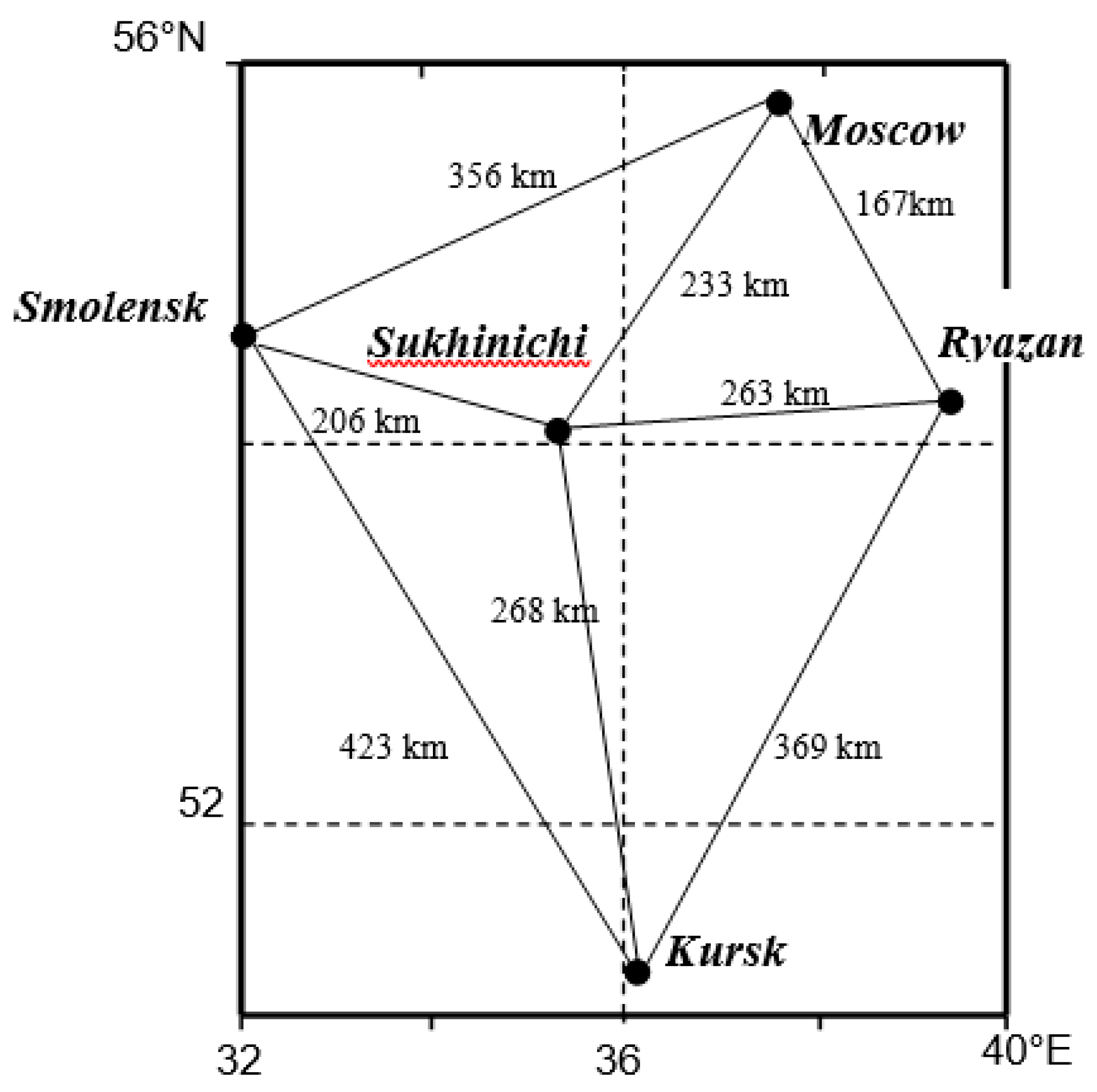
3.1. Description of the Experimental Data

The mesoscale spatial interpolation algorithms discussed above were tested for meteorological ranges of various sizes. The experiment was based on the data obtained in 2015 in the area limited by the mesoscale, which included five upper-air stations: Ryazan, Moscow, Kursk, Sukhinichi, and Smolensk (Figure 1). The Moscow and Kursk weather stations were chosen as reference points for interpolation. Based on the algorithms, the spatial distribution of a cloud of pollutants was numerically analyzed using orthogonal wind velocity components and temperature, averaged within the upper-air layer. The averaging was performed using the expression $<\xi {>}_{h_0,h}$ (here, h₀ is the ground height above sea level, and h is the height of the upper boundary of the layer), for atmospheric layers: 0–200, 0–400, 0–800, 0–1200, 0–1600, 0–2000, 0–2400, 0–3000, 0–4000, 0–5000, 0–6000 and 0–8000 m. Thus, the observations were based on the average values of temperature $<\mathrm{T}{>}_{h_0,h}$, zonal $<\mathrm{U}{>}_{h_0,h}$, and meridional $<\mathrm{U}{>}_{h_0,h}$ wind velocity components for the layer, which were calculated using the actual measurements taken at standard isobaric levels in the height range from 0 to 8 km [21,22].

3.2. Initial Conditions for LKF Initiation

To initiate the Kalman filter shown in Equations (13)–(15) for each interpolation algorithm, the following initial conditions were defined: $\alpha =0.9$, $1/\beta =1200$, $\gamma =1$, ${\gamma }_1=1$, and ${\gamma }_2=1$ for estimating the temperature, and $\alpha =0.3$, $1/\beta =700$, $\gamma =0.5$, ${\gamma }_1=0.5$, and ${\gamma }_2=0.5$ for estimating the orthogonal wind velocity components. The matrices $x_0^a=0$ and $P_0^a=10$ were selected as initial conditions for the state parameters. The main diagonal of the observation noise covariance matrix $R_k={\sigma }_{\xi }^2 I$ is defined using values of the elements of the radiosonde error covariance matrix taken from [22]: ${\sigma }_{\xi }=1$ °C for air temperature, and ${\sigma }_{\xi }=1$ m/s for the orthogonal wind velocity components. The state noise covariance matrix $Q_k=I$ was defined as an identity matrix.

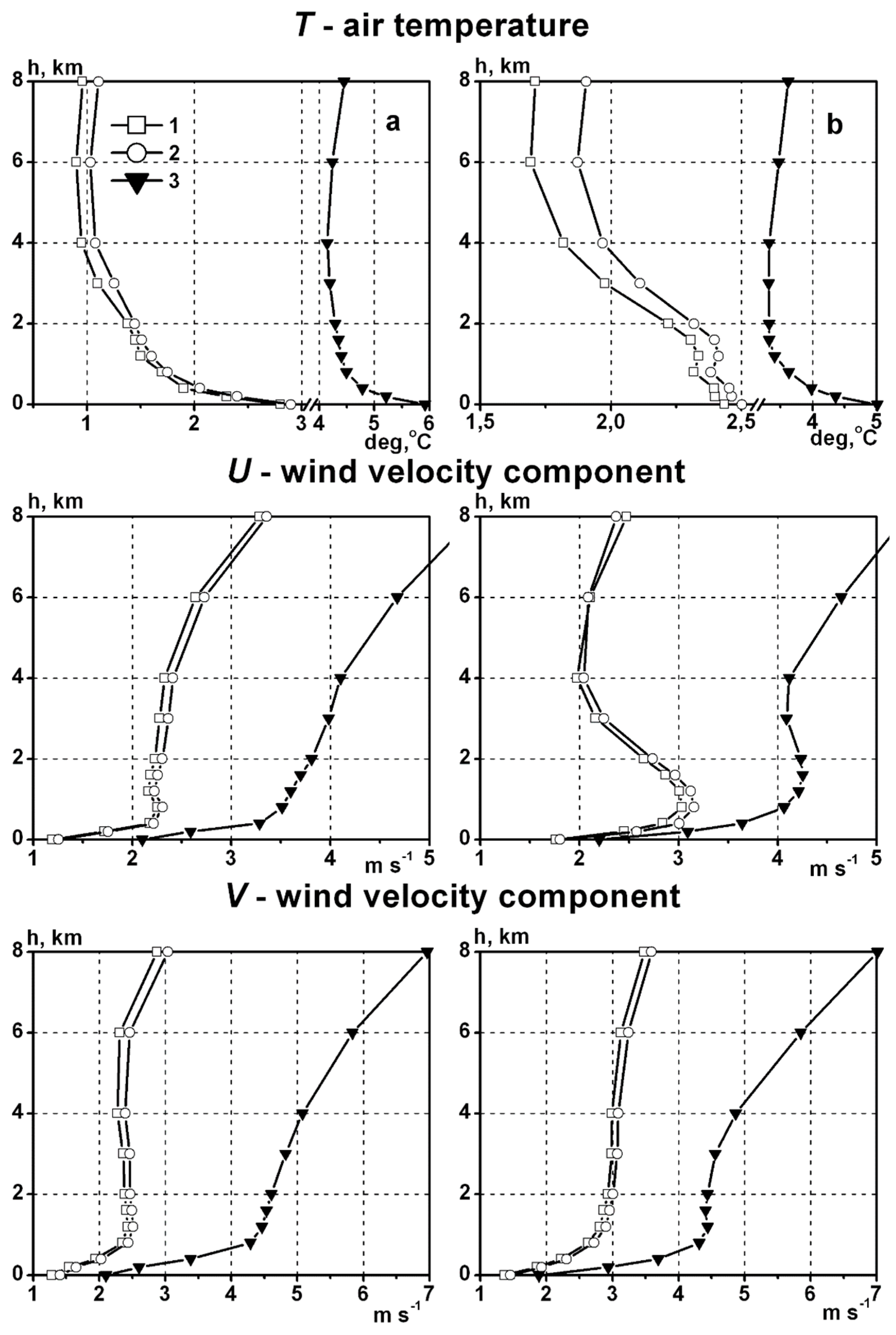
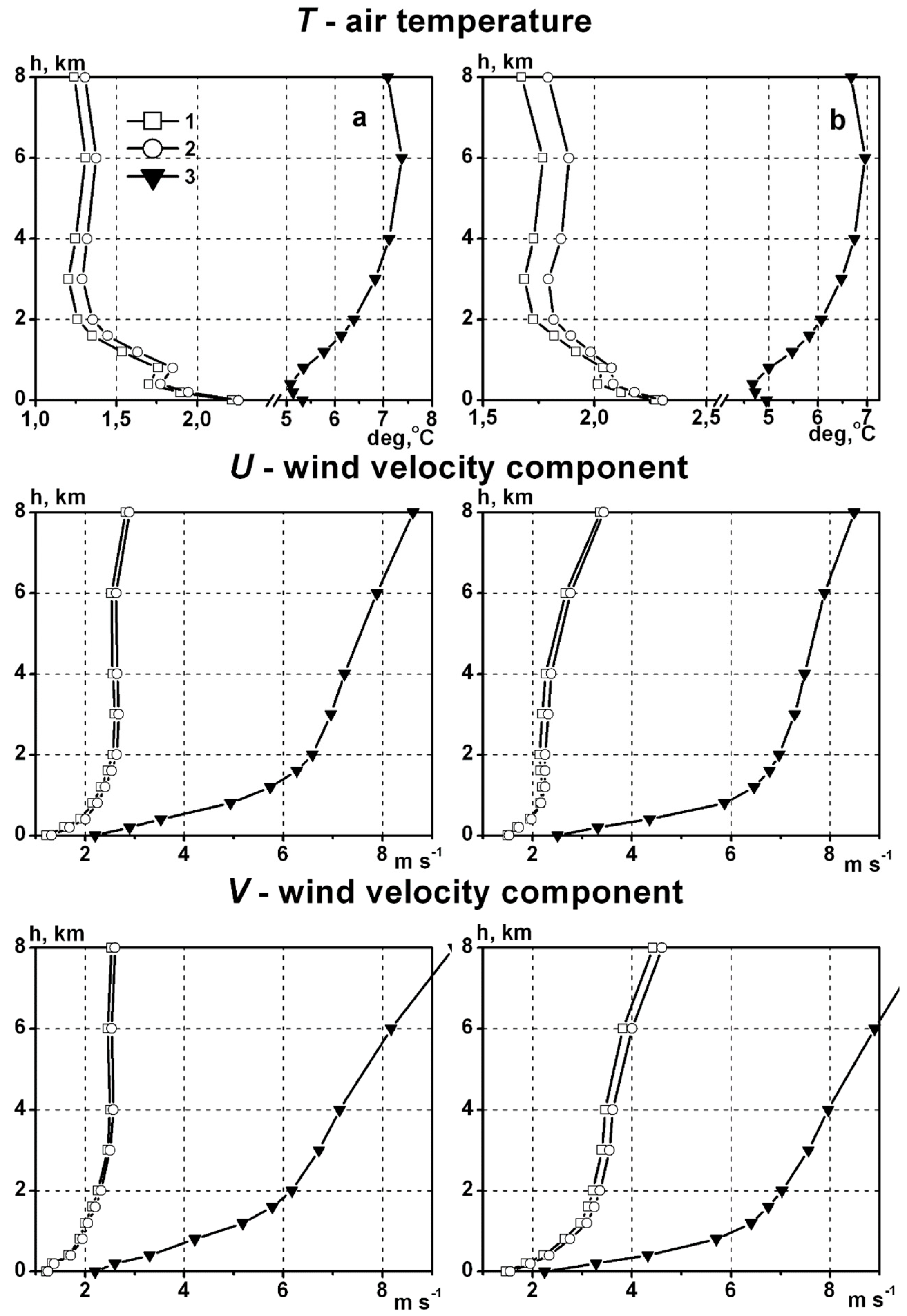
3.3. Comparative Analysis of the Simulation Results

Let us compare the results of numerical simulation for the two spatial interpolation algorithms. It should be noted that the algorithms were compared under equal conditions.

Figure 2 and Figure 3 show behavior graphs for the spatial interpolation (extrapolation) of RMS errors for air temperature, and orthogonal (zonal and meridional) wind velocity components obtained for summer and winter seasons at Kursk and Moscow measuring stations.

The analysis of the graphs suggests that the proposed algorithms can be successfully applied in practice, since the RMS errors of spatial interpolation T, U, and V vary in the range of 0.8–2.5 °C (for air temperature) and 1.0–4.5 m/s (for orthogonal wind velocity components), depending on the height range and season.

The research results show that the proposed algorithms have comparable characteristics in terms of interpolation accuracy. The difference in the accuracy is about 0.1–0.3 °C for air temperature and 0.1–0.5 m/s for wind velocity components.

Thus, the application of the model shown in Equations (3) and (4) in variants (6), (11) or (8), (12) is not necessary for the synthesis of the interpolation algorithm. In any case, the accuracy of the interpolation is comparable.

3.4. Additional Notes

It should be noted that the simulation is based on the pre-calculated coefficients $\alpha$, $\mathsf{\beta }$, and $\gamma$. The parameters of the model in Equations (3) and (4) were set using the empirical correlation functions obtained for each meteorological variable under study (T, V, U) and approximated by exponential expressions $\mu (\tau )=\exp (-\alpha \tau )$, $\mu (\rho )=\exp (-\beta \rho )$, and $\mu (h)=\exp (-\gamma h)$. The calculation technique is well known and considered by the authors in [7].

Obviously, in order to solve operational problems, unknown variables $\alpha$, $\mathsf{\beta }$, and $\gamma$ should be calculated in real time. Two approaches can be used. The first is to introduce unknown variables to be estimated into the state vector. In this case, the problem becomes nonlinear and requires the use of the extended Kalman filter (EKF). The second approach is to use the ensemble Kalman filter (EnKF). Both approaches led to a significant complication of the algorithm structure and require more computation.

The authors are aware that the interpolation algorithms based on a simplified dynamic stochastic model have some limitations. Their application is limited to local areas with a size of not more than 500 × 500 km. Nevertheless, the ease of implementation and the acceptable accuracy of interpolation for a number of applied problems suggest that this approach is applicable to autonomous local networks for collecting meteorological data. In particular, the authors applied these methods to restore a vertical profile of the atmospheric boundary layer using measurements from unmanned aerial vehicles (UAVs). The results suggest that the proposed approach can be successfully used for areas limited by the γ (gamma) and β (beta) mesoscale.

4. Conclusions

In conclusion, it should be noted that the studies of interpolation algorithms based on the Kalman filter and the low-order parametric dynamic stochastic model taking into account the height variation of meteorological fields demonstrate that the presented algorithms are sufficiently effective and can be successfully used to solve applied meteorological problems.

A preliminary estimation of the parameters $\alpha$, $\mathsf{\beta }$, and $\gamma$ should be based on spatial, inter-level, and temporal correlation properties of the atmosphere in a given mesoscale region, which were obtained by processing meteorological and upper-air measurements in real time. This conclusion is supported by the studies of the algorithms with different sets of coefficients $\alpha$, $\mathsf{\beta }$, and $\gamma$ for different values of meteorological variables and heights. The results of these studies allowed us to identify some clear trends and impose relevant requirements. Thus, the further development of the algorithm will be aimed at estimating the parameters of the model based on both EKF and EnKF.

From the point of view of software implementation, the algorithm using the first variant of state and observation Equations (7) and (9) has a smaller dimension of the state vector, and therefore requires less computational cost. It should be noted that this filter provides an estimate of meteorological variables for only one fixed height level. Therefore, in order to restore the entire vertical profile at a forecast point, we need to use several filters that operate simultaneously (in our case, 12 filters operating in parallel). Nevertheless, the scope of computational operations for the first variant (7), (9) is less than that for the second variant (8), (12). This makes the first variant more preferable for practical use.

Due to low requirements for computer memory and performance, the developed algorithms can be used in operational environmental monitoring systems, including those based on mobile platforms. In this regard, using UAVs as a versatile platform that can carry meteorological sensors and provide regular automatic measurements of vertical profiles in the atmospheric boundary layer over areas not covered by measurements is a promising application.

References

1. Bushby, F.H.; Huckle, V.M. Objective analysis in numerical forecasting. Q. J. R. Meteorol. Soc. 1957, 83, 232–247. [Google Scholar] [CrossRef]
2. Belov, P.N. Numerical Methods of Weather Forecasting; Gidrometeoizdat: Leningrad, Russia, 1967; p. 335. [Google Scholar]
3. Gordin, V.A.; Loktionova, E.A. On the application of the spline-approximation of the hydrostatic equation to the checking and adjustment of temperature and height data samples. Res. Act. Atmos. Ocean. Model. 1981, 2, 12–17. [Google Scholar]
4. Gandin, L.S.; Kagan, R.L. Statistical Methods of Meteorological Data Interpretation; Gidrometeoizdat: Leningrad, Russia, 1976; p. 359. [Google Scholar]
5. Gandin, L.S. Objective Analysis of Meteorological Fields; Gidrometeoizdat: Leningrad, Russia, 1963; p. 287. [Google Scholar]
6. Komarov, V.S. Statistics in Application to Solve Applied Meteorological Problems; Publishing House “Spektr” of IAO SB RAS: Tomsk, Russia, 1997; p. 256. [Google Scholar]
7. Komarov, V.S.; Popov, Y.B.; Suvorov, S.S.; Kurakov, V.A. Dynamic-Stochastic Methods with Their Application to Meteorology; Publishing House of IAO SB RAS: Tomsk, Russia, 2004; p. 236. [Google Scholar]
8. Popov, Y.B.; Popova, A.I. Optimum Filtering and Its Application in Tasks of Monitoring of State Parameters of Atmosphere within the Bounds of Local Areas; Polygraphist: Khanty-Mansiysk, Russia, 2008; p. 188. [Google Scholar]
9. Klimova, E.G. Recovering Meteorological Fields from Observational Data. Doctor Thesis, Institute of Computational Technologies of SB RAS, Novosibirsk, Russia, 2005. [Google Scholar]
10. Klimova, E.G. A suboptimal data assimilation algorithm based on the ensemble Kalman filter. Q. J. R. Meteorol. Soc. 2012, 138, 2079–2085. [Google Scholar] [CrossRef]
11. Houtekamer, P.L.; Mitchell, H.L. Data assimilation using an ensemble Kalman filtering technique. Mon. Weather Rev. 1998, 126, 796–811. [Google Scholar] [CrossRef]
12. Schlatter, T.W. Variational assimilation of meteorological observations in the lower atmosphere: A tutorial on how it works. J. Atmos. Sol. Terr. Phys. 2000, 62, 1057–1070. [Google Scholar] [CrossRef]
13. Wilks, D.S. Statistical Methods in the Atmospheric Sciences, 2nd ed.; Academic Press: Cambridge, MA, USA, 2006; p. 611. [Google Scholar]
14. Lavrinenko, A.V.; Moldovanova, E.A.; Mymrina, D.F.; Popova, A.I.; Popova, K.Y.; Popov, Y.B. Spatial interpolation of meteorological fields using a multilevel parametric dynamic stochastic low-order model. J. Atmos. Sol. Terr. Phys. 2018, 181 Pt A, 38–43. [Google Scholar] [CrossRef]
15. Popov, Y.B. Estimation of atmospheric state parameters using the four-dimensional dynamic-stochastic model and Kalman linear filter. Part 1. Methodical foundations. J. Proc. TUSUR 2010, 21 Pt 2, 5–11. [Google Scholar]
16. Klimova, E.G. A primitive-equation model for calculation of forecast error covariances in the Kalman filter algorithm. Russ. Meteorol. Hydrol. 2001, 11, 5–12. [Google Scholar]
17. Marchuk, G.I. Numerical Methods in Weather Prediction; Academic Press: Cambridge, MA, USA, 1974; p. 288. [Google Scholar]
18. Zverev, A.S. Synoptic Meteorology; Gidrometeoizdat: Leningrad, Russia, 1977; p. 711. [Google Scholar]
19. Komarov, V.S.; Popov, Y.B. Estimation and prediction of atmospheric state parameters using the Kalman filtering algorithm. Part 1. Methodic foundation. J. Atmos. Ocean. Opt. 2001, 14, 230–234. [Google Scholar]
20. Komarov, V.S.; Il’in, S.N.; Kreminskii, A.V.; Lomakina, N.Y.; Popov, Y.B.; Popova, A.I.; Suvorov, S.S. Estimation and extrapolation of the atmospheric state parameters on the mesoscale level using a Kalman filter algorithm. J. Atmos. Ocean. Technol. 2004, 21, 488–494. [Google Scholar] [CrossRef]
21. Komarov, V.S.; Lavrinenko, A.V.; Lomakina, N.Y.; Popov, Y.B.; Popova, A.I.; Il’in, S.N. Spatial extrapolation of mesoscale meteorological fields using a 4D-dynamic-stochastic model and the Kalman filter algorithm. J. Atmos. Ocean. Opt. 2004, 17, 651–656. [Google Scholar]
22. Komarov, V.S.; Lavrinenko, A.V.; Kreminskii, A.V.; Lomakina, N.Y.; Popov, Y.B.; Popova, A.I. New method of spatial extrapolation of meteorological fields on the mesoscale level using a Kalman filter algorithm for a four-dimensional dynamic-stochastic model. J. Atmos. Ocean. Technol. 2007, 24, 182–193. [Google Scholar] [CrossRef]
23. Evensen, G. The Ensemble Kalman Filter: Theoretical formulation and practical implementation. Ocean Dyn. 2003, 53, 343–365. [Google Scholar] [CrossRef]
24. Wang, S.; Ancell, B.C.; Huang, G.H.; Baetz, B.W. Improving Robustness of Hydrologic Ensemble Predictions Through Probabilistic Pre- and Post-Processing in Sequential Data Assimilation. Water Resour. Res. 2018, 54, 2129–2151. [Google Scholar] [CrossRef]
25. Bishop, C.H.; Etherton, B.J.; Majumdar, S.J. Adaptive Sampling with the Ensemble Transform Kalman Filter. Part I: Theoretical Aspects. Mon. Weather Rev. 2001, 129, 420–436. [Google Scholar] [CrossRef]
26. Whitaker, J.S.; Hamill, T.M. Ensemble data assimilation without perturbed observations. Mon. Weather Rev. 2002, 130, 1913–1924. [Google Scholar] [CrossRef]
27. Ott, E.; Hunt, B.R.; Szunyogh, I.; Zimin, A.V.; Kostelich, E.J.; Corazza, M.; Kalnay, E.; Patil, D.J.; Yorke, J.A. A local ensemble Kalman Filter for atmospheric data assimilation. Tellus 2004, 56A, 415–428. [Google Scholar] [CrossRef]
28. Szunyogh, I.; Kostelich, E.; Gyarmati, G.; Kalnay, E.; Hunt, B.R.; Ott, E.; Satterfield, E.; Szunyogh, I.; Yorke, J.A. A local ensemble transform Kalman Filter data assimilation system for the NCEP global model. Tellus 2007, 59A, 1–18. [Google Scholar]
29. Zupanski, M. Maximum Likelihood Ensemble Filter: Theoretical Aspects. Mon. Weather Rev. 2005, 133, 1710–1726. [Google Scholar] [CrossRef]
30. Sage, A.P.; Melsa, J.L. Estimation Theory with Application to Communication and Control, 1st ed.; McGraw-Hill: New York, NY, USA, 1971; p. 752. [Google Scholar]
Figure 1. Diagram of the meteorological proving ground.
Symmetry 11 01207 g001
Figure 2. Vertical distributions of the root mean square (RMS) spatial interpolation (extrapolation) errors on air temperature, as well as zonal and meridional wind velocity components, based on a low-order parametric model with a vertical component for first (1) and second (2) variant of design, and the corresponding vertical profiles of the standard deviations (3), for Moscow (a) and Kursk (b) stations. Summer.
Symmetry 11 01207 g002
Figure 3. Vertical distributions of the RMS spatial interpolation (extrapolation) errors on air temperature, as well as zonal and meridional wind velocity components, based on the low-order parametric model with a vertical component for the first (1) and second (2) variant of design, and the corresponding vertical profiles of the standard deviations (3), for Moscow (a) and Kursk (b) stations. Winter.
Symmetry 11 01207 g003