Efficient Vehicle Detection and Distance Estimation Based on Aggregated Channel Features and Inverse Perspective Mapping from a Single Camera

Abstract

In this paper a method for detecting and estimating the distance of a vehicle driving in front using a single black-box camera installed in a vehicle was proposed. In order to apply the proposed method to autonomous vehicles, it was required to reduce the throughput and speed-up the processing. To do this, the proposed method decomposed the input image into multiple-resolution images for real-time processing and then extracted the aggregated channel features (ACFs). The idea was to extract only the most important features from images at different resolutions symmetrically. A method of detecting an object and a method of estimating a vehicle’s distance from a bird’s eye view through inverse perspective mapping (IPM) were applied. In the proposed method, ACFs were used to generate the AdaBoost-based vehicle detector. The ACFs were extracted from the LUV color, edge gradient, and orientation (histograms of oriented gradients) of the input image. Subsequently, by applying IPM and transforming a 2D input image into 3D by generating an image projected in three dimensions, the distance between the detected vehicle and the autonomous vehicle was detected. The proposed method was applied in a real-world road environment and showed accurate results for vehicle detection and distance estimation in real-time processing. Thus, it was showed that our method is applicable to autonomous vehicles.

1. Introduction

In recent years, interest in autonomous vehicles has been increasing rapidly. Traditional vehicles can be improved with advances in artificial intelligence and its applications in various fields. Automakers are developing self-driving vehicles and are selling vehicles with safe driving devices to support the driver. For safe autonomous driving, a fusion of various technologies is needed along with vehicle IT technology [1,2,3,4]. For vehicle IT technology, the sensors include laser, radar, ultrasonic wave, lidar, charge coupled device (CCD) sensors, and additional devices for communication among vehicles. However, sensors for the safe driving of vehicles remain expensive. An additional problem is that sensors can be easily damaged in slight collisions [5,6]. Moreover, sensors that collect three-dimensional information (such as lidar) are not practical for common use, because the price of a sensor is comparable to the price of a vehicle [3,7]. Therefore, ultrasonic sensors are used to collect two-dimensional information to recognize nearby objects as an auxiliary device for safe driving. However, most of these sensors are located on the outside of the vehicle (front and rear bumper and rearview mirror). In some cases, sensors may malfunction because of the damage caused by an external collision or the presence of dust. In recent years, most vehicles have been equipped with black-box devices to record driving conditions [6,8,9,10]. In some countries, black boxes are mandatory for business vehicles or are installed with government support [6]. Currently, black-box devices for vehicles are used to recover information only in special situations, such as vehicle accidents. Therefore, it was required to develop a black box for a vehicle equipped with a function of automatically recognizing the driving situation in advance and automatically providing relevant information for the driver to support safe driving. Some of the existing video recording devices include a driver assistance function (such as a lane departure and a departure guide on the front side) [6,8,9,10,11,12,13]. However, it has a very limited capacity for supporting driving safety because it cannot detect and estimate the distance of objects 50 m or beyond in all directions. Therefore, we proposed a technique of estimating the distance between the vehicle and other vehicles in real-time, by using an image acquired from a low-cost image-recording device.

Many studies based on vision sensors have been carried out for vehicle detection and symmetrical distance estimation [14,15,16,17]. Image processing can be applied in different ways based on the features of the vision sensor. By detecting the vehicle on the input image using image processing, various information about the detected vehicle can be obtained. Vehicle detection research includes, for example, feature-based template matching methods [18,19,20,21,22], neural networks or support vector machines [23,24,25], or shape- and motion-based methods [19,26,27]. Vehicle detection methods are mostly based on features that assume an invariable and formal shape of the vehicle. Vehicle-to-vehicle distance estimation research includes a distance estimation method based on the size of the detected vehicle [15,17,28], stereo camera-based method [16,29], and a method that compares the size of road infrastructure (lane, guide rail, etc.). Vehicle distance estimation methods are mostly based on the detected vehicle shape information [12]. Although the distance estimation based on the stereo camera provides a relatively accurate result, the stereo camera is more expensive, and the computation throughput is more limited than for a mono camera.

Therefore, in this paper, I proposed a method to detect a forward moving vehicle from a single camera and to estimate the distance of the current vehicle from the detected vehicle. To reduce computational cost and ensure symmetrical real-time processing, the input road image was decomposed into multiple-resolution images, and vehicle detection was performed for a low-resolution image. The proposed method used a cascade classifier using aggregated channel features (ACFs) and the AdaBoost algorithm [30,31] to learn vehicle images and generate vehicle detectors. The AdaBoost algorithm is known as a classifier that can classify two classes well by adaptive boosting. The AdaBoost algorithm is an improved method to use the idea of boosting algorithm in real data analysis. It generates a strong classifier with a combination of several week classifiers and weight values. The Adaboost algorithm re-adjusts the weight of the sample data at the beginning of learning; the data are equally weighted but misclassified data increase the weight difference and well-classified data decrease the weight. The classifier with the lowest weighted error value at each stage is one weak classifier. The Viola-Jones algorithm [32] is known as an effective real-time object detection algorithm using the AdaBoost algorithm using square features as a weak classifier.

In the proposed method, the ACFs are used to downsample a multi-resolution image without reducing the feature information included in the input image. The ACF is a method that reduces the original image size by downsampling it, while maintaining unique features of the image and skipping other features. Thus, ACF aims to reduce the dimensions of the image and maintain unique features at the same time. After all, two-dimensional feature information is extracted and downsampled k times to generate kth feature information while maintaining (k−1)th feature information. This has the advantage of reducing the amount of computation [33]. In the proposed method, ACF and AdaBoost algorithms [32,34] are used to learn the automotive domain in advance for vehicle detection. The reason for using the AdaBoost algorithm is that it is about 15 times faster than the study using neural networks or SVM (support vector machine), and has high accuracy, as Viola [32] revealed.

Subsequently, an inverse perspective transformation (IPM) was applied to estimate the distance from the detected vehicle region in the input image [35,36]. Inverse perspective transformation is a method of generating a bird-view (or top-view) image by projecting a two-dimensional image acquired by a camera into a three-dimensional real-world space and mapping it to a two-dimensional space again. Although it is impossible to accurately calculate the distance with image-based processing, the experiments showed that the distance error was within ±5 m for moving vehicles. To apply the proposed method to the safe driving support system of a vehicle under a road driving environment, real-time processing was required. In our method, the image size was reduced while maintaining the feature information of the input image, and then the vehicle was detected using an AdaBoost-based vehicle detector. Afterwards, using the inverse perspective transformation, the two-dimensional road image was mapped onto the three-dimensional space that corresponded to the real-world space, and the distance to the detected vehicle was estimated symmetrically.

1.1. Related Works

Kim et al. [13] used Haar-like features and edge orientation information to detect vehicles, and they used the detected vehicle widths and location information to estimate the distance among vehicles. To build a classifier that can detect vehicles, a large number of vehicle images is required for training. To overcome this difficulty, they used the pattern of the rear part of the vehicle on the road to detect the vehicle. However, if the surface of the vehicle reflects sunlight or if objects that are not related to the vehicle (such as road pollution or lanes) are included in the road image, misdetection may occur. To use the width of the detected vehicle for the estimation of the vehicle distance, it is required to accurately detect the shape of the vehicle.

Jeong et al. [37] proposed a method to detect a vehicle and estimate the distance to prevent collision. They proposed a method that uses Haar-like features to detect driving vehicles. To estimate the distance, the method uses the number of horizontal pixels of the detected vehicle area. Candidate vehicle regions are selected using Haar-like features, and only vehicle regions are detected in the candidate vehicle regions according to the shape of the edge distribution through the Sobel edge. The distance to the detected vehicle was estimated using a pre-trained distance database that calculates the actual number of pixels per meter. This method has the disadvantage of low accuracy because it does not consider changes in image resolution and the degree of distortion of the camera in actual calculations. In addition, the estimated distance database (DB) is calculated up to 15 m, which limits its application in real-world road environments.

Bertozzi et al. [29] proposed a method of projecting a two-dimensional image onto a three-dimensional real world through computation of inverse perspective transformation to estimate the distance to the vehicle detected in the image acquired from the camera. However, projecting a two-dimensional image onto a three-dimensional space is challenging for real-time processing, because the amount of calculations is increased per pixel.

In order to implement a safe ADAS, Lee et al. [38] and Yin et al. [39] proposed a method for analyzing a driver’s movement while driving and focusing on a driving task. In their proposed method, the risk level was estimated using the hand movement information of the driver. While their methods are concerned with the inadvertent driving behavior of the driver, the proposed method proposes a method that is interested in the movement of other vehicles.

1.2. Definition of Problems

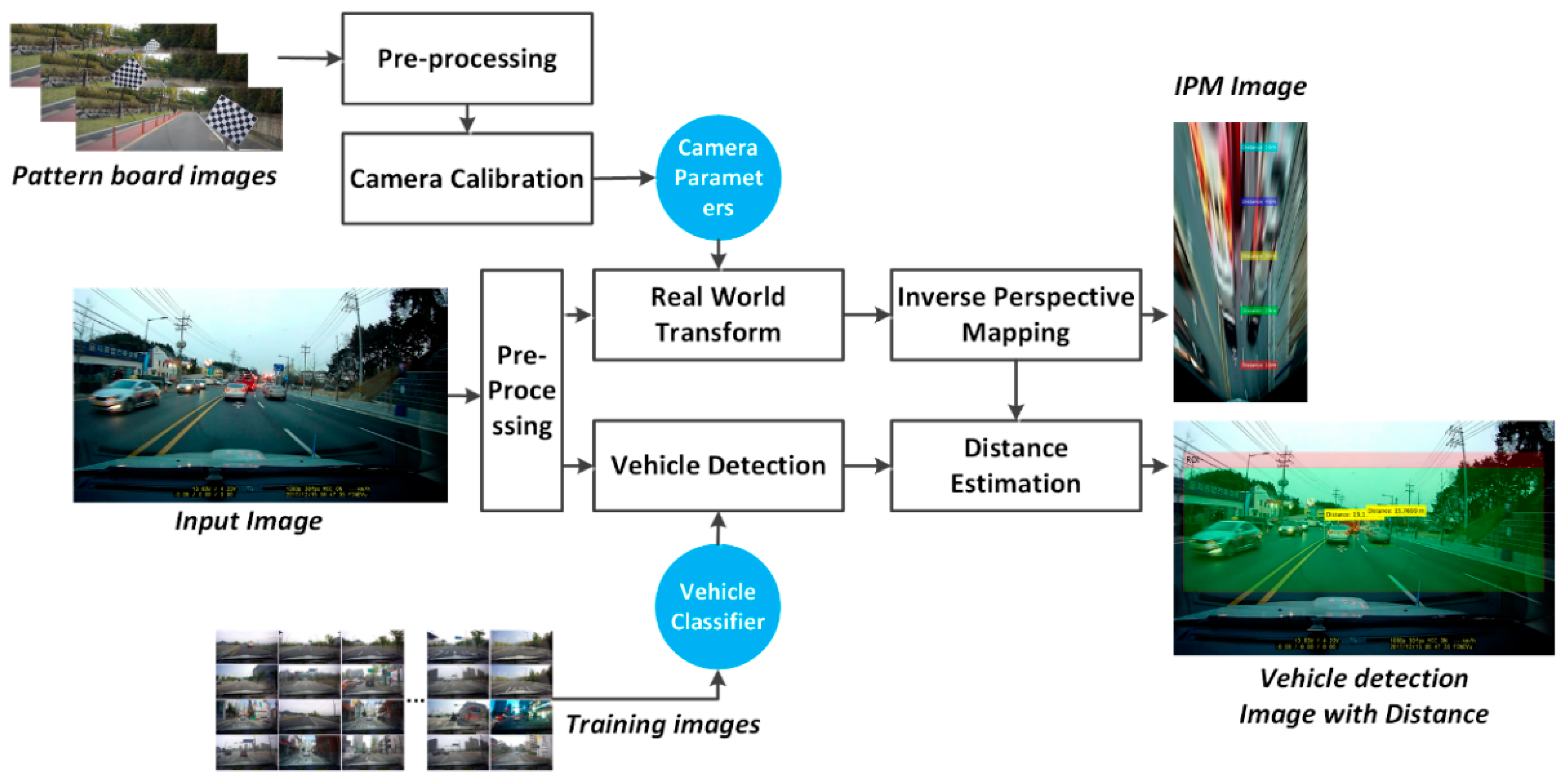
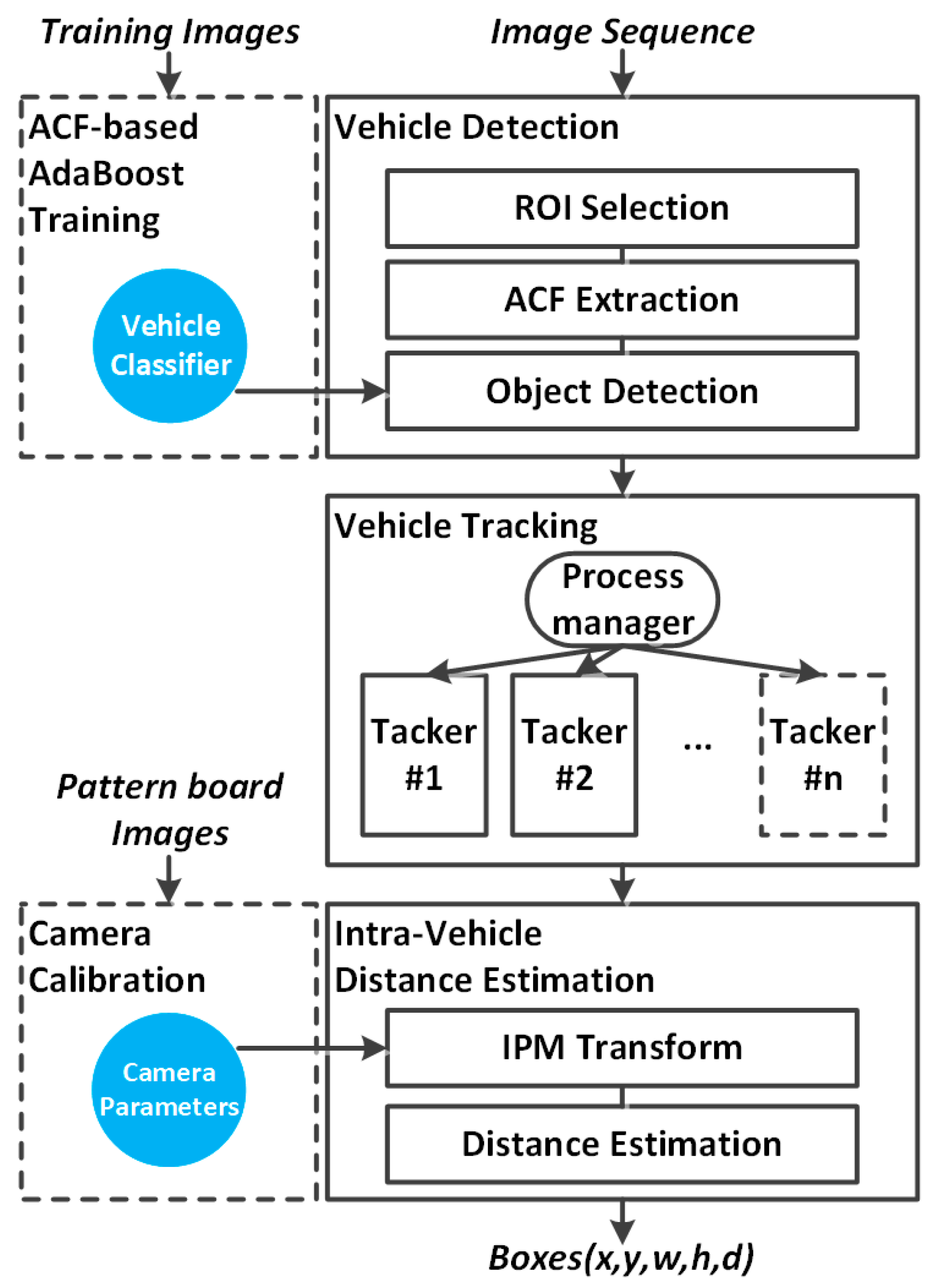
To ensure vehicle safety, detection of a vehicle moving forward in road environment requires real-time processing. The storage capacity of the black-box camera used in the proposed method is more than 30 frames per second. However, it is difficult to process more than 10 frames per second because of the high computational complexity of the image processing algorithm for vehicle detection and inter-vehicle distance estimation. Therefore, a problem in this study was that the computational complexity increased with the increase in the dimensions of the input image. As a result, the calculation time required for image processing increased. As proposed by Dollar et al. [30], several well-refined image features can be extracted, and these features can be enhanced to improve detection performance. However, it is difficult to process more than 15 frames per second because of an increased amount of pixel calculations. As in the autonomous driving and safe driving support system to be applied in the proposed method, a vehicle detection and inter-vehicle distance estimation of more than 10 frames per second were required to ensure a relatively high accuracy at the speed of 60 km/h. To guarantee the satisfaction of these processing constraints in this problem area, it was necessary to select whether or not to reduce the processing of more than 10 frames per second instead of increasing the accuracy of the vehicle detection by applying complex features. Furthermore, it was necessary to estimate the distance among vehicles in real-time and to implement the method without additional sensors (ultrasonic, lidar, stereo vision, etc.). Therefore, in this paper, the problems of vehicle detection and distance estimation are defined as follows. The detection of the target vehicle is limited to vehicles in the same driving lane. The distance estimation is limited by the vehicles within 70 m ahead. To achieve real-time processing and a relatively high accuracy, it is necessary to apply a method that can effectively extract unique features and reduce computational complexity, even if the dimensions of the input image is reduced.

2. Proposed Methods

Figure 1 shows the workflow of the proposed method for vehicle detection and distance estimation based on road images when driving forward symmetrically. The proposed method includes three processing steps: vehicle detection, tracking, and distance estimation. Additionally, two preliminary steps are required for this workflow: learning the vehicle images and extracting the camera parameters. Figure 2 shows the process of vehicle detection and distance estimation. In the pre-processing step, the 1920 × 1080 pixel size was reduced to a 900 × 505 pixel size, and the median filtering process was performed to remove the salt and pepper noise included in the road image. In the vehicle detection step, the regions of interest (ROI) corresponding to the vehicle detection area was first selected in the input image. Next, the ACFs were extracted from the ROI and the vehicles were detected using the ACF-based vehicle detector. It was possible not only to process the entire input image for detecting the vehicle but also to reduce computations by performing the detection step only in the region of interest. Next, vehicle regions detected by the vehicle detector were tracked through a pixel-matching process. Finally, the distance of the current vehicle from the detected vehicle was estimated (during the vehicle distance estimation step) based on the center coordinates of the bounding box area of the detected vehicle. In the proposed method, the inverse perspective transformation method was applied to transform the input image into a three-dimensional space to estimate the actual distance to the vehicle.

In this paper, I propose a vehicle detection method, a car tracking method, and a car distance estimation method in Section 3, Section 4 and Section 5, respectively. Next, the experimental results are shown in Section 6. Finally, the paper is concluded in Section 7.

3. Vehicle Detection

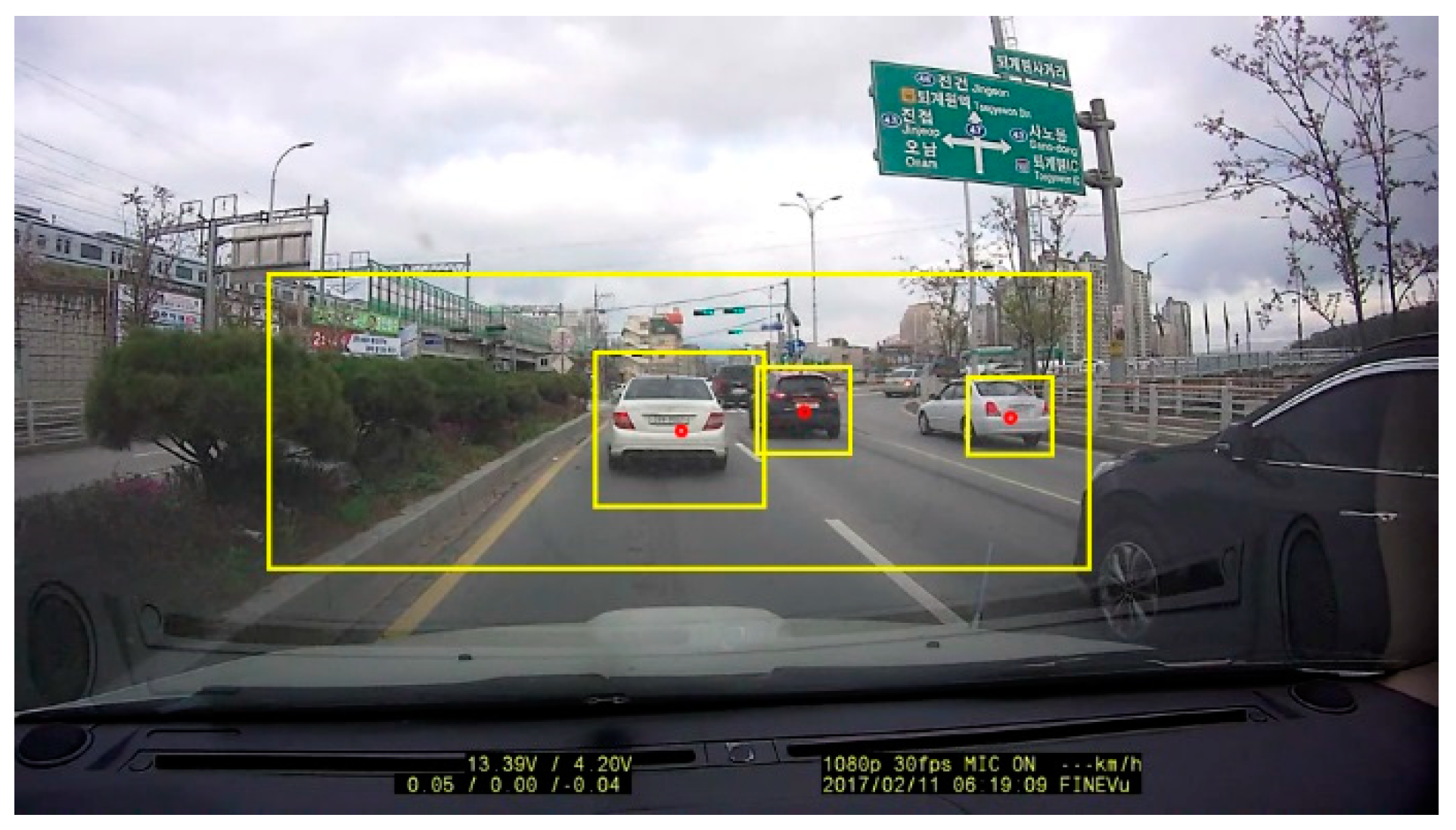
3.1. ROI Selection

To detect vehicles in the input image, it is necessary to reduce the detection processing range. This step is required to provide vehicle detection information in real time to enable safe driving support. Therefore, in the proposed method, ROI was selected from the input image. In the problem definition, the selection of the ROI includes the left and right lanes of the driving lane, as it determines the range of the detection and distance estimation of the vehicle traveling in the same road lane. Moreover, the ROI for the vehicle detection was selected from the center part of the image obtained from the moving vehicle. The ROI can be selected without any processing by applying a pre-defined pixel size filtering on the input image, to reduce the execution time. However, when the ROI includes a bus or truck with a height of approximately 3 m or more, part of the vehicle is omitted in the ROI, thus the vehicle is not be detected. After selecting the ROI for the vehicle detection process, the ACFs were extracted from the detected area of the vehicle in the ROI, and the vehicle was detected by inputting it into a previously trained vehicle detector.

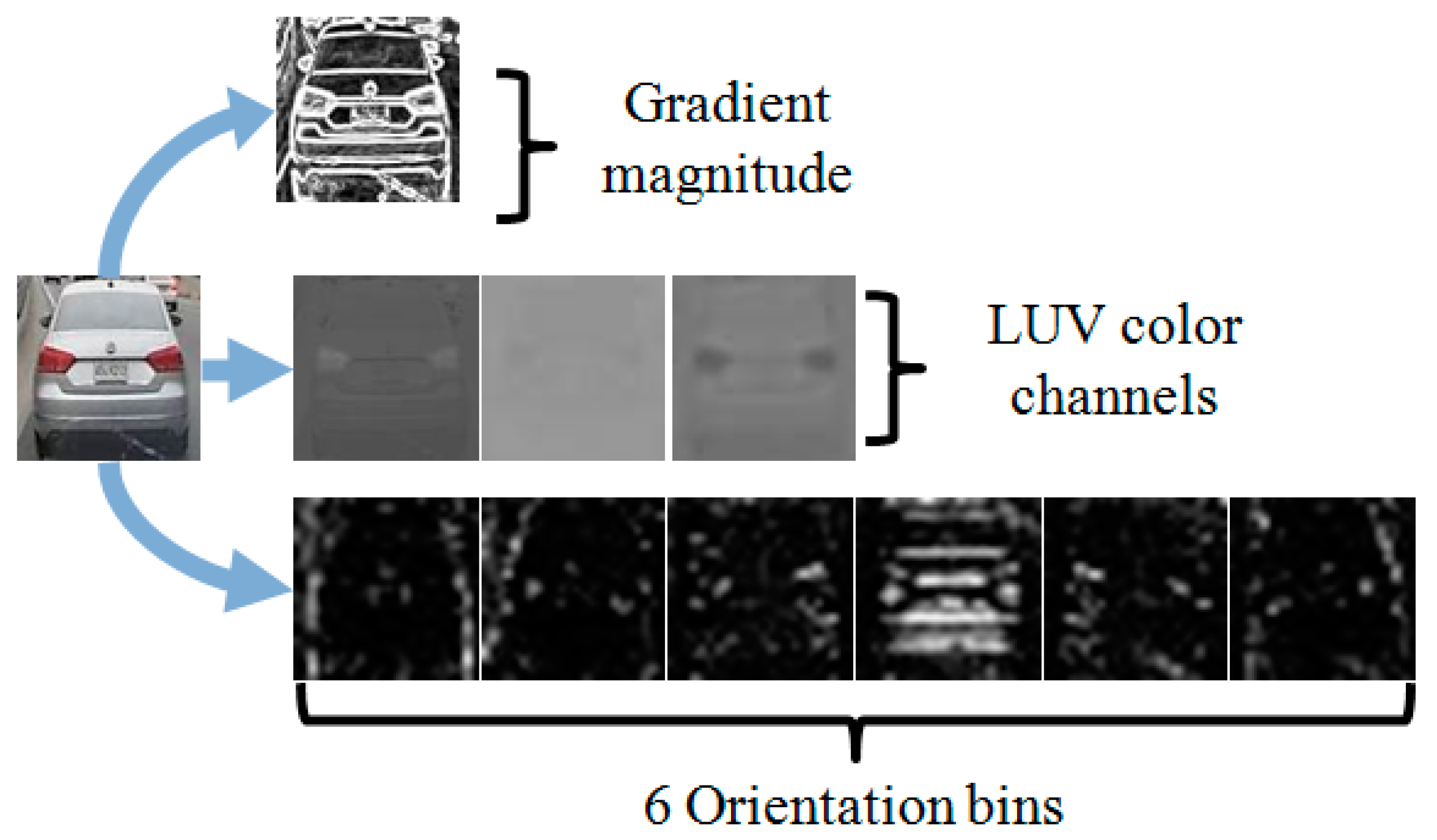
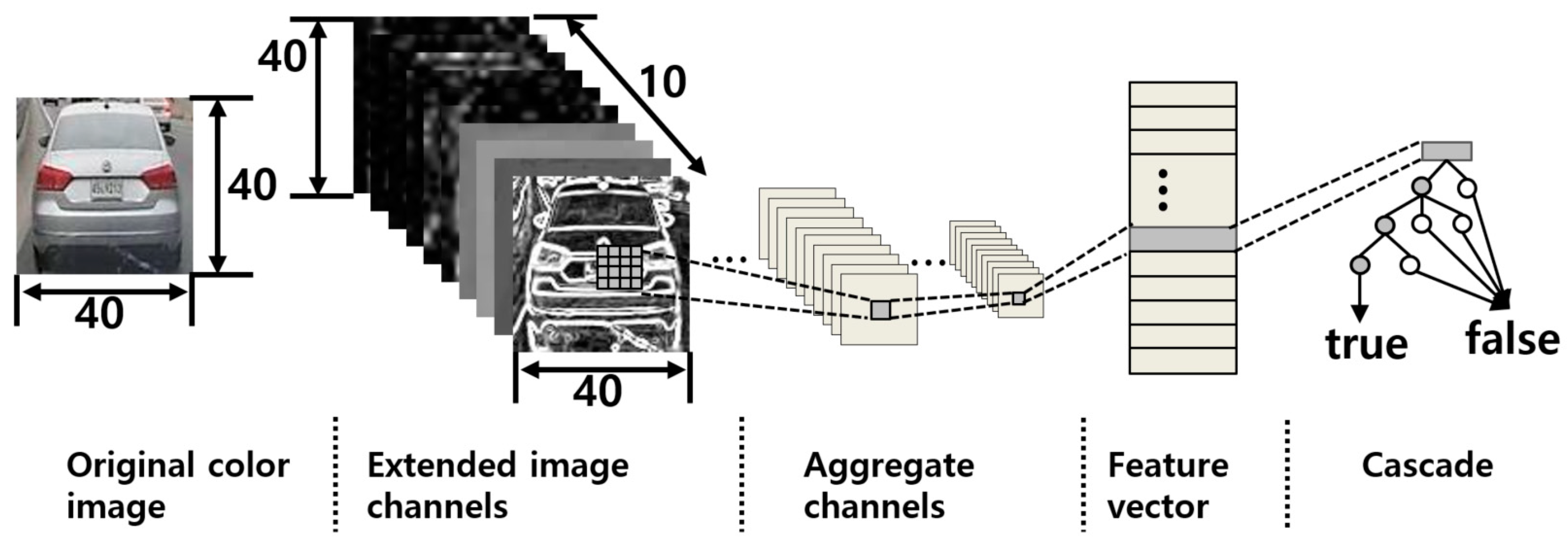
3.2. Extraction of Aggregated Channel Features

Dollar et al. [30] proposed the ACFs to dramatically enhance the performance of pedestrian detection. The ACFs have the characteristic of extracting unique features quickly from the image. To quickly extract the ACFs, the input image was first generated as a multiple-resolution pyramid of images at a high speed. For the images included in the pyramid, the feature information was extracted, including the same and uniquely extracted features from the high-level resolution image to the low-level resolution image. The process of extracting ACFs was as follows. After extracting feature information from the input image, the kth feature information was generated, while the (k−1)th feature information was maintained while downsampling k times. That is, the ACFs have a characteristic of keeping the (k−1)th extracted feature information, even if it is the kth downsampled extracted feature information.

Therefore, it is possible to extract the unique features of an input image even from a low-resolution image (in which the dimensions are reduced) without processing the input image; thus, the amount of calculations can be reduced [29,30].

Among features used in existing object detection studies, Haar-like [40,41,42] and integral channel features (ICFs) [43,44] extract features from fixed-size blocks. However, the ACFs proposed by Dollar et al. [30] have the advantage of extracting characteristic information regardless of object size variations (by extracting features from blocks of various sizes). The input RGB image (I) was calculated as a total of ten feature channels (C = Ω (I)) as shown in Figure 3. Each feature channel included a normalized gradient magnitude, a quantized gradient angle in six orientations, and LUV color channels. Each feature channel was calculated by a 4 × 4 pixels block sum, reduced four times, and smoothed by a (1/4 1/2 1/4) filter. Finally, the feature vectors were extracted from the feature space of the low-level resolution multi-channel decomposition of the input image. Subsequently, a classification process was performed to distinguish whether the extracted feature vectors belong to the object of interest. To classify the ACFs of the object of interest, this step used a binary decision-tree-based classifier to generate a strong classifier. Among the ACF channels, the LUV color model focused on the fact that human beings are more visually sensitive to intensity than color. The L channel is the brightness value, the U channel is red and green, and the V channel is blue and purple [45]. The process of recalculating the RGB color model as the LUV color model is shown in Equation (1). Here, X_n, Y_n, and Z_n are white color information. Figure 4 shows a flowchart of the vehicle detector processing based on ACF.

$$\begin{array}{l}\left[\begin{array}{c}X\\ Y\\ Z\end{array}\right]=\left[\begin{array}{ccc}0.607& 0.174& 0.200\\ 0.299& 0.587& 0.114\\ 0.000& 0.066& 1.116\end{array}\right]\left[\begin{array}{c}R\\ G\\ B\end{array}\right]\\ U^{\prime }= \frac{4X}{X+15Y+3Z^{\prime }}\\ V^{\prime }= \frac{9Y}{X+15Y+3Z^{\prime }}\\ U_n^{\prime }= \frac{4X_n}{X_n+15Y_n+3Z_n^{\prime }}\\ V_n^{\prime }= \frac{9Y_n}{X_n+15Y_n+3Z_n^{\prime }}\\ L= \{\begin{array}{c}116{\left(\frac{Y}{Y_n}\right)}^{\frac{1}{3}}-16, if \frac{Y}{Y_n}>0.008856\\ 903.3\frac{Y}{Y_n} , Other\end{array}\\ U=13L\left(U^{\prime }-U_n^{\prime }\right), U=13L\left(V^{\prime }-V_n^{\prime }\right)\end{array}$$

(1)

3.3. Object Detection

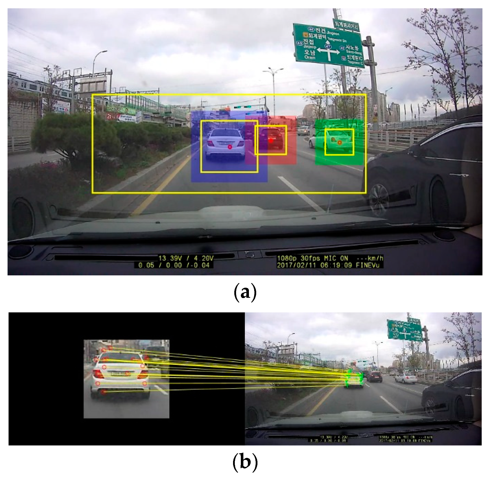
In this step, the vehicle is detected in the input image using the ACF-based vehicle detector. The vehicle detector extracts ACFs from training images in advance and combines it with an AdaBoost-based learning algorithm to generate a strong classifier. The AdaBoost algorithm is a method of binary classification through matching process based on features of training images. The ACFs extracted from the vehicle and non-vehicle training images are matched and can be used to distinguish the two classes. The mutual matching process of features is performed not only once, but also on various conditions. As a result, these multiple conditions are composed of weak classifiers by generating a strong classifier with a linear combination of weak classifiers. The resulting classifier can quickly produce a result with a good accuracy. In other words, a strong classifier is generated that provides high accuracy through linear combinations of weak classifiers that correctly classify learned features.

Table 1. Overview of the AdaBoost algorithm.

Step 1. Define learning data: m objects of interest (+1) and n non-objects of interest (−1):

$\left(x_1,y_1\right), \dots , \left(x_i,y_i\right),i=1, \dots , N,N=m+n$ $x_i\in \left\{training samples\right\}, y_i\in \left\{1, -1\right\}$

Step 2. Initialization of the weight value of i-th weak classifier (h):

$weigt{h}_i^1=\{\begin{array}{c}\frac{1}{m}, y_i=-1 \\ \frac{1}{n}, y_i=+1\end{array}$

Step 3. Training step (repeat for t = 1, …, C, t++)

(1) Normalization of the weight value of the i-th learning sample of the t-th weak classifier:

$weigt{h}_i^t=\frac{weigh{t}_i^t}{{{\displaystyle \sum }}_{i=1}^{N}weigh{t}_i^i}$

(2) Calculation of error rate (${\epsilon }_t$) of t-th weak classifier:

${\epsilon }_t={\displaystyle {\displaystyle \sum }_{i=1}^N}weigh{t}_i^t\left|h_t\left(x_i\right)-y_i\right|$

(3) Selection of a weak classifier (h) with a minimum error rate.

(4) Updating weight values:

$weigt{h}_i^{t+1}=weigt{h}_i^t\times \{\begin{array}{c}{e}^{-{\alpha }_t}, if h_t\left(x_i\right)=y_i \\ e^{{\alpha }_t}, if h_t\left(x_i\right)\ne y_i\end{array}$ ${\alpha }_t=log\frac{1}{{\beta }_t}, {\beta }_t=\frac{{\epsilon }_t}{1-{\epsilon }_t}$

Step 4. Creation of a strong classifier (H(x)) as a linear combination of weak classifiers (h):

$H\left(x\right)=sign\left({\displaystyle {\displaystyle \sum }_{n=1}^C}{\alpha }_n{h}_n\left(x\right)\right)$

describes the AdaBoost algorithm.

To create an AdaBoost-based vehicle detector, the first step is to collect a training dataset N that represents two classes: images with vehicles (m, class: +1) and images without vehicles (n, class: −1). In the second step, the weight of the training data(x) are initialized to the same value. It is possible to select strong classifiers by updating weight values iteratively in the learning process. In the third step, the learning data are fed to the weak classifier. Subsequently, the error rate between the predicted result and the previously known result is calculated. To calculate the learning error rate, the weight value of the learning data is first normalized. The error rate is a total sum of values obtained by multiplying the learning data values erroneously classified in the learning data by the weight values. Here, the error rate means the probability of presenting misclassified results in the classifier’s learning process. Therefore, it is necessary to adjust the weight values assigned to them to exclude weak classifiers that present the results that are misclassified in the learning process. Therefore, the weak classifiers correctly presented by the learning result, that is, classifiers exhibiting a low error rate, are selected. If the tth weak classifier is correctly classified as the label of the learning data, the error (${\epsilon }_t$) becomes small. As a result, ${\alpha }_t$ increases, and the weight value becomes small. If the weight value of the tth weak classifier becomes smaller, the probability that a weak classifier with a smaller weight value is selected in the next learning process becomes higher, thereby reducing the probability of misclassifying the learning data. Finally, the final step is to create a strong classifier that can correctly classify the learning data as a linear combination of weak classifiers with a low misclassification probability [46]. Figure 5 shows examples of images used for training the vehicle detector. The images show the rear part of the front vehicle that was driving in various road environments. The ACFs were extracted from the training image, and the extracted information was converted into a feature vector and used as an input to the AdaBoost-based vehicle classifier. The vehicle image detected by the classifier is shown in Figure 6. Generally, a large amount of training images is required to improve the performance of the vehicle detector.

The proposed method has a disadvantage if a large amount of training images cannot be obtained. Therefore, to reduce the possibility of false detections of vehicles, the detection region was verified by using some preliminary information. The proposed method used additional information to verify that the vehicle was included in the area detected by the vehicle detector. This information included the position of the detected region, the aspect ratio of the detected region, the ratio of the average brightness of the learning vehicle regions to the brightness of the detected vehicle region, and vehicle template. To determine whether the vehicle was included in the detected region, the information applied in the proposed method was determined as the final vehicle region by comparing the position, aspect ratio, average brightness, and the vehicle template. The vehicle averaging template was an image accumulated by normalizing the learning vehicle region to 31 × 34 pixels and converting it to gray color.

Table 2. Criteria of vehicle region verification.

Criteria	Method
position (x, y, width, height)	position = [25, 101, 846, 267]
aspect ratio (width/height)	0.6939 <= ratio <= 13.1700
brightness Ratio (avrIntensity)	0.3563 <= avrIntensity <= 3.7889
vehicle template	template >= 0.7

shows the criteria for verifying the presence of the vehicle in the region detected by the vehicle detector. Each validation criterion value determines whether it is the vehicle (according to whether it is included in the range).

4. Vehicle Tracking

At this step, the vehicle regions (previously detected in the vehicle detection step) are tracked through a pixel-matching process [47]. Based on the feature information contained in the detected vehicle region, the vehicle region is tracked by performing a comparison process, specifically, by searching for adjacent regions that have the most similar feature information. In the proposed method for reducing the pixel-matching processing time, a range for comparison with the most similar regions in the adjacent frames was set. Generally, in an image obtained at a speed of 15 frames per second, the position of a moving vehicle was less than approximately 20 pixels in an adjacent frame. Therefore, the region of 20 pixels was set as the center of interest in the vehicle region detected in the vehicle detection step. Pixel matching was performed in the corresponding region in the adjacent frame. Figure 7 shows the results of vehicle tracking through the pixel matching process in the detected vehicle region.

5. Vehicle Distance Estimation

At this step, we estimated the distance of the current vehicle from the detected vehicle. To estimate the distance, we used the inverse perspective transformation method [35]. The input image was projected to a real-world image through inverse perspective transformation. Next, the distance between the actual camera and the detected vehicle was estimated from the image projected in three dimensions. The distance estimation method was processed as shown in Figure 2. The camera calibration process was performed to acquire the parameters of the camera in advance. Through this process, information such as the focal length of the camera, degree of distortion, and lens bending rate were obtained. The inverse perspective transformation method transforms a two-dimensional image into a three-dimensional space image that has a perspective using camera parameters. Finally, the real-world coordinates were calculated to estimate the distance between the camera and the pixels of the actually detected vehicle region on the inverse perspective transformed three-dimensional space.

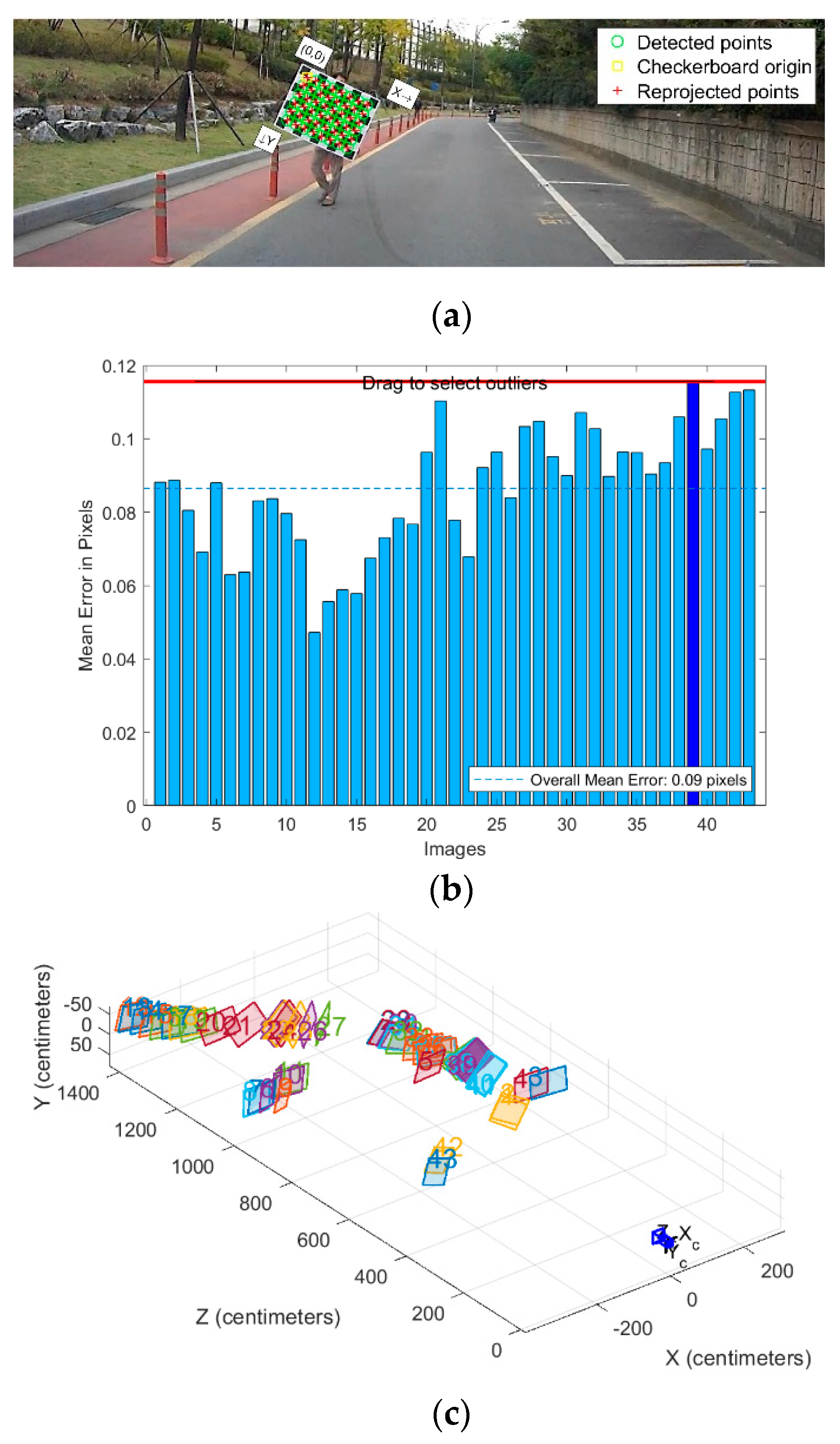
5.1. Camera Parameters Extraction

At this step, we extracted the parameters of the vehicle’s black-box camera. In most cases, a vehicle black-box camera was installed to acquire an omnidirectional road image from a driver’s point of view. In other words, it was installed depending on the visual sensation without going through the accurate measurement for the black-box camera installation. Therefore, an accurate acquisition of the parameters of the black-box camera was required to estimate the distance from the vehicle. Camera parameters included the degree of image warping, tilt and rotation angle, installation height, and focal length of the camera lens. To calculate these parameters, it was necessary to analyze the environment in which the image was acquired. In the proposed method, the camera parameters were calculated using pattern board images. Figure 8 shows the results of estimating the camera parameters in the checkerboard pattern image. Camera calibration is the process of estimating parameters of the camera using images in a checkerboard pattern, and the reprojection error is calculated using the calibration image. The reprojection error is the distance between the checkerboard pattern detected in the calibration image and a world point projected on the same image. The calibration image with a high mean reprojection error was excluded. Figure 8c shows the location of the checkerboard pattern images using camera parameters in real-world space.

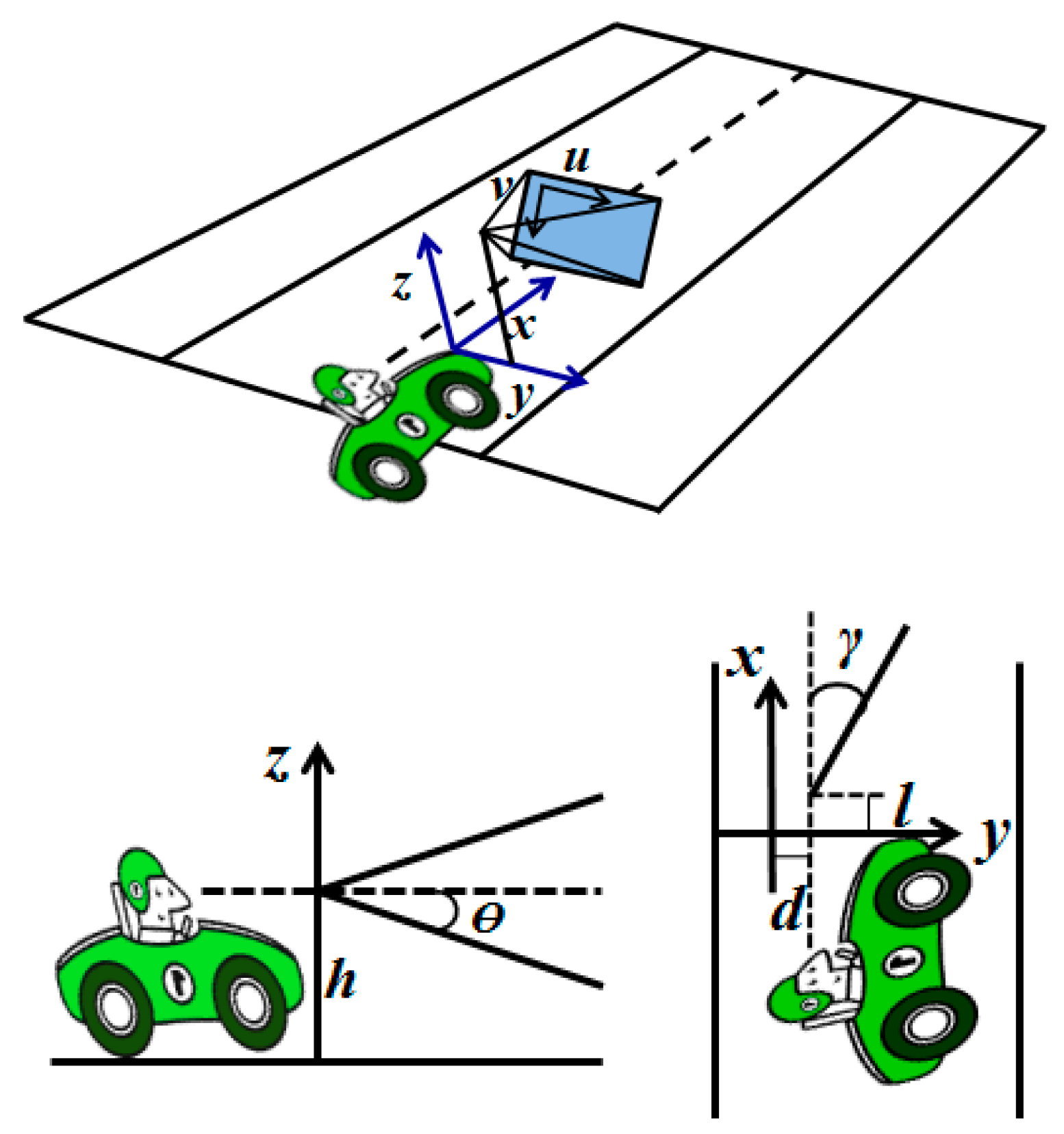
5.2. Inverse Perspective Transformation

As shown in the previous research [29,35], a 2D image obtained from a vehicle black-box camera contains the perspective effect and stores it. The perspective effect means that the coordinates of three-dimensional space (x,y,z) are mapped to two-dimensional space (u,v). Therefore, the two-dimensional image loses perspective information in the real world, and the inverse perspective transformation re-estimates the information about the perspective through the calculation process. As shown in Figure 9, when the three-dimensional coordinate system is mapped to the two-dimensional coordinate system, information about the image acquisition camera is required to estimate the perspective information. To transform the three-dimensional real-world coordinate system from two-dimensional images, the proposed method acquires the angle of camera view (α), installed height (h), twist degree (r: top-down camera angle, θ: horizontal camera angle), size of the input image (n × m), and location information of the camera (l and d). Next, the obtained values were substituted into Equation (2) to generate a two-dimensional image that included the perspective [48].

In the proposed method, position (d, l) of the camera was set to 1. The height (h) of the camera at the ground was set to 1.8. The left and right rotation (r, θ = 0) of the camera was set to 0. Figure 10 shows the result of a bird-view image mapping a 2D image to a 3D real-world image.

$$\begin{array}{l}x\left(u,v\right)=h tan\left[\left(\overline{\theta }-\alpha \right)+u\frac{2\alpha }{n_u-1}\right]\times cos\left[\left(\overline{\gamma }-\alpha \right)+v\frac{2\alpha }{n_v-1}\right]+l\\ y\left(u,v\right)=h tan\left[\left(\overline{\theta }-\alpha \right)+u\frac{2\alpha }{n_u-1}\right]\times sin\left[\left(\overline{\gamma }-\alpha \right)+v\frac{2\alpha }{n_v-1}\right]+d \\ z\left(u,v\right)=0\end{array}$$

(2)

6. Experimental Results

To validate the proposed method, experimental images were obtained from a vehicle black-box camera in real-world road conditions at various times. The images obtained for the experiment were 1920 × 1080 pixels in the HD-class black-box image.

The experimental setup was a PC with Windows 10 OS (3.3 GHz Hexa Core, 48 GB RAM, dual 1080Ti GPUs) and MATLAB. To reduce the processing time, the size of the input image was reduced to 900 × 505 pixels by the bilinear interpolation method. In the proposed method, the number of positive vehicle images used for training of the AdaBoost algorithm was 2256 and non-vehicle images were selected for the remaining area that excluded the vehicle regions. The average size of the training vehicle regions for the vehicle detection was 31 × 34, the repetition period (T) of the AdaBoost algorithm is set to 4, the number of training samples in the non-vehicle (negative) for each learning step was 2 (S: 2), and the maximum number of weak classifiers was set to 2048. (It is necessary to measure errors according to each setting.)

As shown in Figure 11, the proposed method was evaluated by comparing precision (P) and recall (R), as in Equation (3). Accuracy shows how often the vehicle detector provides correct results, and the recall rate is an indicator of how much the detector actually detects the vehicle. In other words, the accuracy (P) measures how accurately the vehicle area is detected, and the recall rate (R) is a measure of how much the area deviates from the detected vehicle area.

$$P=\frac{M_m{{\displaystyle \cap }}^{ }{M}_o}{\left(M_m{{\displaystyle \cap }}^{ }{M}_o\right)+M_o}, R=\frac{M_m{{\displaystyle \cap }}^{ }{M}_o}{M_m+\left(M_m{{\displaystyle \cap }}^{ }{M}_o\right)}$$

(3)

Here, $M_m$ and $M_o$ are the region previously specified as ground-truth in the learning stage and the vehicle region detected by the vehicle detection algorithm, respectively.

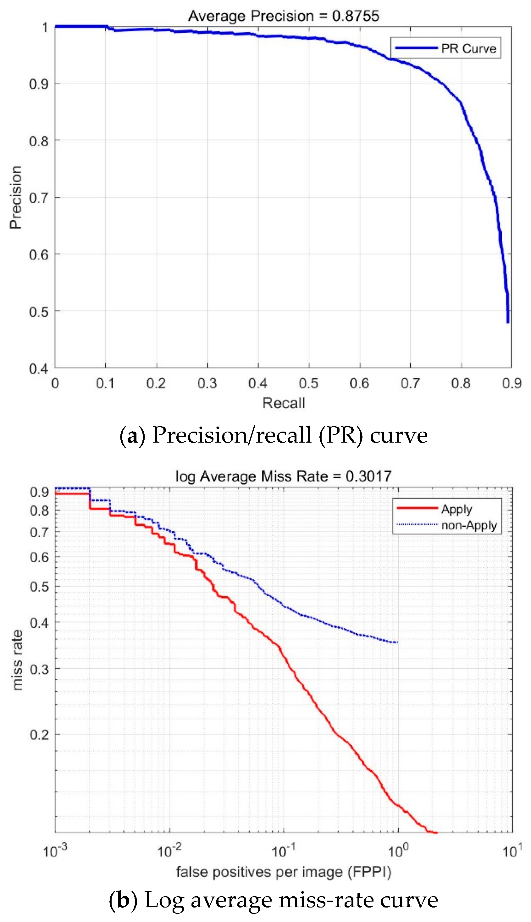
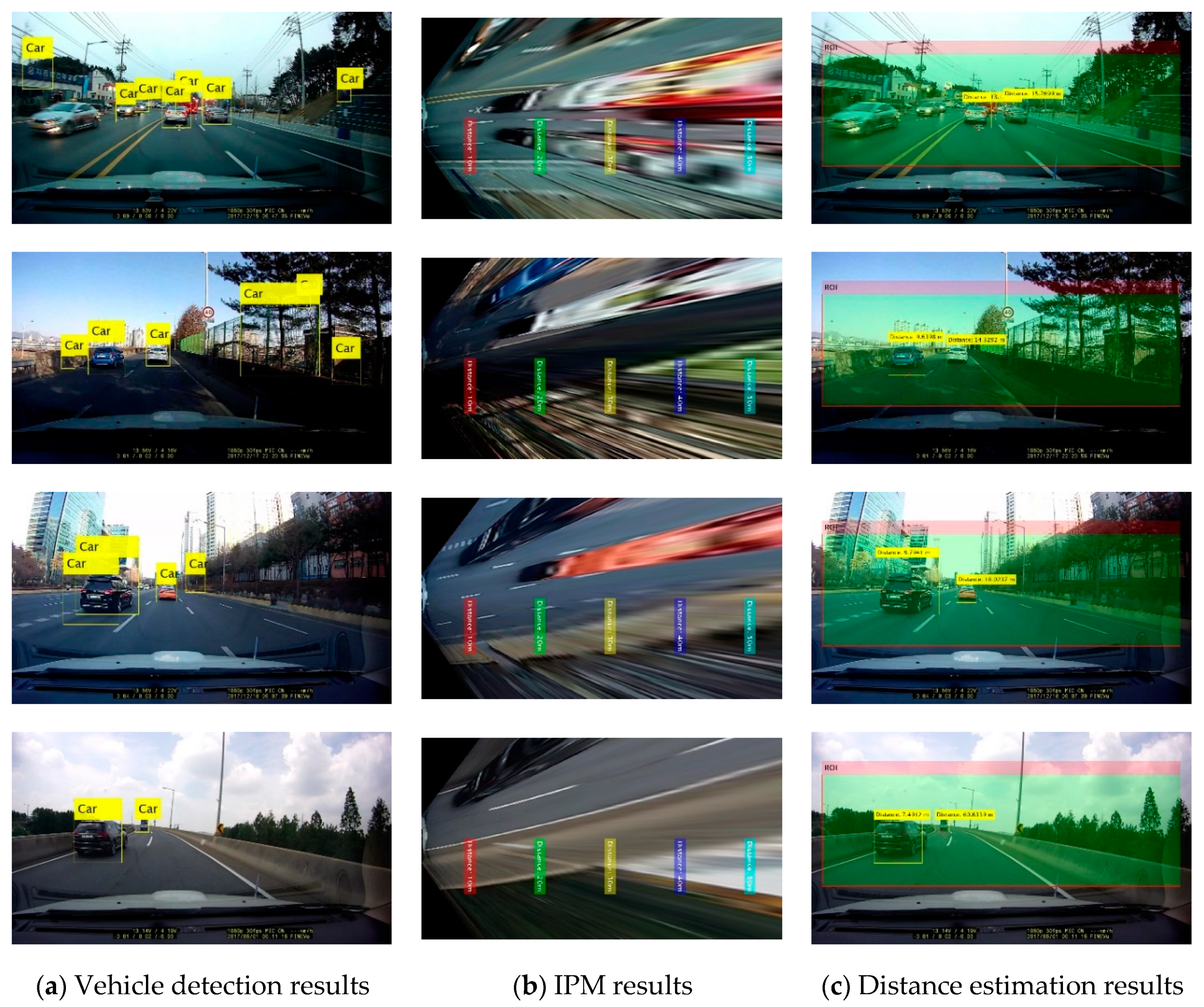
6.1. Results of Vehicle Detection

To evaluate the performance of the proposed vehicle detection method, we compared the vehicle region selected by the ground-truth method and the vehicle region detected by the proposed method using Equation (3). The performance of the proposed vehicle detector was evaluated using precision and recall. To determine the parameters of the AdaBoost algorithm for the vehicle detector, we analyzed the accuracy and recall according to the number of learning cycles and training samples. To evaluate the performance of the vehicle detector, the threshold value for a correct vehicle detection was set to 0.5 according to the degree of overlap between the vehicle region selected by the ground-truth method and the vehicle region detected by the proposed method. If more than half of the selected vehicle region was detected in the experiment, it was judged as correct vehicle detection.

Figure 12a shows the average detection accuracy as a receiver operating characteristic (ROC) curve that measures how accurately a true positive sample was classified according to the learning cycle and the sampling factor of the non-vehicle region. Figure 12b shows the ROC curve of the log average vehicle detection error rate according to the vehicle verification step. The detection error rate (MR: miss rate) means the mis-detected rate, and the false positive per image (FFPI) means the number of mis-detected regions of the image.

Table 3. Experimental results for an average vehicle detection accuracy, error rate, and learning time requirements according to the vehicle detector setting parameters (T: learning cycle, S: non-vehicle area sampling factor).

	Measures	Average Precision	Log Average Error Rate	Training Time (s)
Parameters
T = 2, S = 2		0.7847	0.4917	283.57
T = 2, S = 4		0.5791	0.6387	432.47
T = 4, S = 2		0.8755	0.3017	592.30
T = 4, S = 4		0.8422	0.2947	680.04
T = 5, S = 2		0.8428	0.2901	751.25
T = 5, S = 4		0.8433	0.2908	821.34
T = 6, S = 2		0.8292	0.3161	1257.56
T = 6, S = 4		0.8375	0.2906	1503.33

shows the average vehicle detection success rate and learning time according to the negative sampling factor (S) versus the learning period (T) required to train a vehicle detector. In the experiment, it was possible to obtain the optimum learning period (T) and the sample factor (S) for generating the vehicle detector.

Table 3 shows that even if the learning success cycle (T) and the non-car area sample factor (S) for generating the car detector in the learning process were set to T = 4 and S = 2, it can be seen that the success rate of the detection of the vehicle did not significantly change, regardless of the time consumed. Experimental results show that the average detection accuracy of the vehicle was 87.6% and the average execution time was 0.051 s. The learning period (T) and the sample factor (S) were set to values with high vehicle detection accuracy and minimum learning time. In the proposed method, T and S were set to 4 and 2, respectively. It can be seen that even if learning was performed by setting a higher value, the success rate of the vehicle detection did not change much, even though the learning time increased.

Table 4. Results of the vehicle detection with various features.

	Measures	Average Precision	Recall (R)	Average Processing Time, (s)
Features
Haar		0.7310	0.4941	0.135
LBP		0.7641	0.5634	0.126
HOG		0.8375	0.4775	0.149
Our methods		0.8755	0.3017	0.121

shows the results of vehicle detection according to the features and the learning algorithm used for vehicle detection. We compared the following features with the proposed method [41]: Haar, local binary patterns, and Histogram of Gradient (HOG). Additionally, the learning algorithm used in the vehicle detector was compared with the vehicle detection results of the cascade learning algorithm.

To learn the configuration parameters of Haar, LBP, and HOG-based cascade learners [34], we set the learning area size to 31 × 34, false alarm rate to 0.1, negative sampling factor to two, and learning cycle to six. The performance comparison of the vehicle detection results was classified as the correct detection if the degree of overlap between the detected vehicle region and the actual vehicle region was 50% or more. Results of vehicle detection based on various features showed that the proposed approach outperforms the method that used other features.

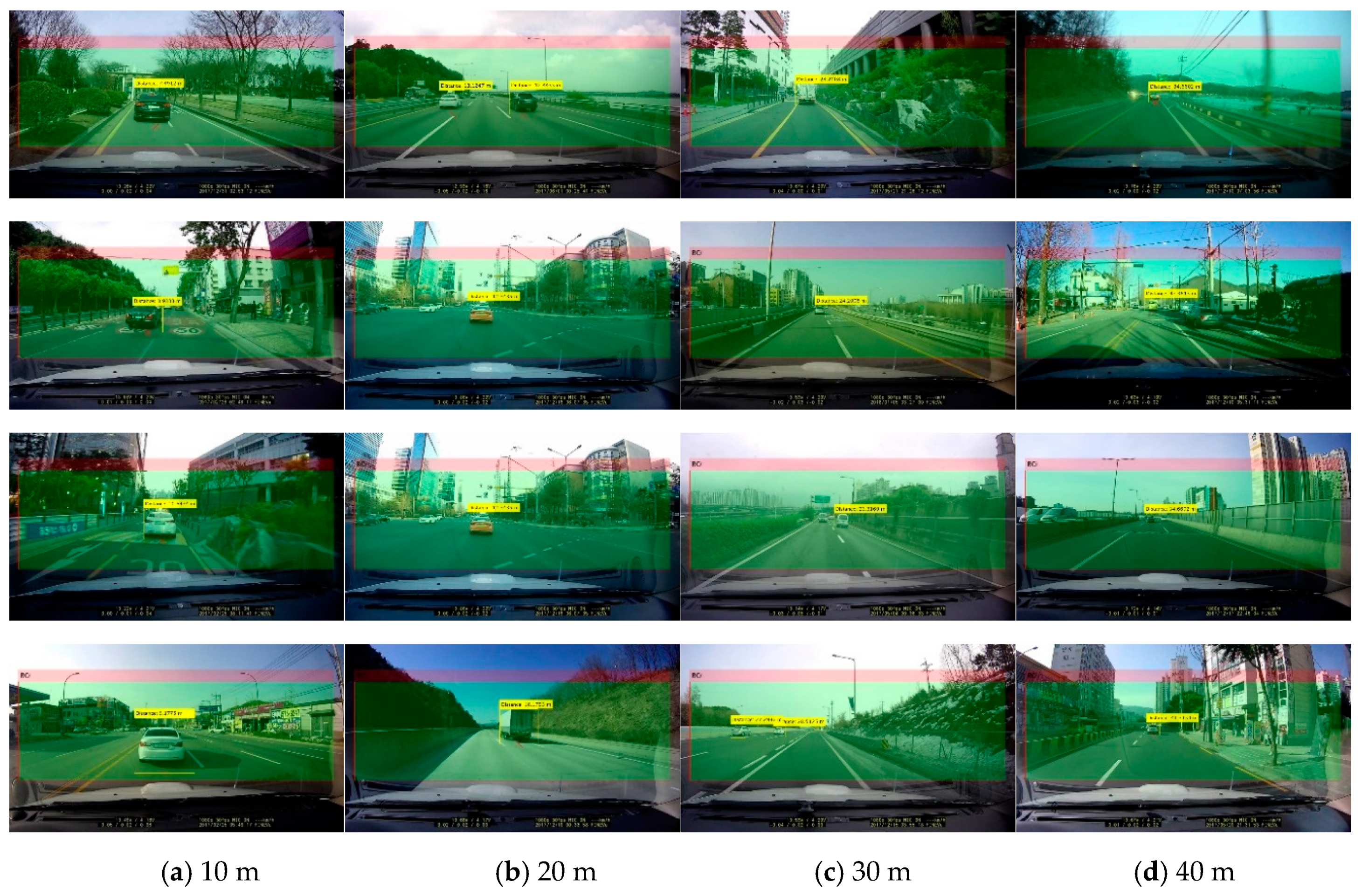
6.2. Results of Vehicle Distance Estimation

To evaluate the performance of the vehicle distance estimation method, the proposed method was compared with the distance estimation results by using experimental images showing distances of up to 50 m in 10 m increments in 10 different road environments. In addition, we compared the results measured using the laser range finder with the accuracy of the proposed method. Figure 13 shows the results of estimating the distance to the vehicle detected in various road environments.

Table 5. Results of the detected vehicle distance estimation.

	Measure	Average Distance Estimation (m)	Accuracy (%)
Distance
10 m		9.8	98.0
20 m		21.7	92.2
30 m		32.7	91.7
40 m		43.8	91.3
50 m		54.8	91.2

shows the distance estimation results and the distance estimation accuracy of the proposed method for 10 experimental images for each distance. The results show that the detection rate of the vehicle was approximately 87.5%, and the accuracy of the distance estimation rate was approximately 92.8%. The execution time required to process an image was approximately 0.76 s. In the proposed method, the processing time was consumed by performing inverse perspective transformation for every input frame. Future research will be conducted to reduce the distance estimation time using a stereo camera to obtain 3D information without inverse perspective transformation. Figure 14 shows the results of the vehicle detection and distance estimation using the proposed method in a real road environment. Figure 14a shows the results of vehicle detection in the input image, (b) shows the range for the template matching to track the vehicle, and (c) shows the results of detecting the final vehicle region through the vehicle verification process in the detected vehicle regions and the distance estimation result.

7. Conclusions

The proposed method estimates the distance between the current vehicle and the detected vehicle ahead from the image obtained from the black-box camera installed in the vehicle. In the proposed method, the ACF-based AdaBoost algorithm was used to detect the vehicle region and estimate the distance to the vehicle detected using the inverse perspective transformation symmetrically.

In the experiments on various road environments, the accuracy of the vehicle detection was estimated to be 87.5%, the accuracy of the distance estimation was 92.8%, and the time required for the processing was 0.76 s per frame. In the experimental road environment, there was a problem of misdetection when the driving vehicles overlapped with the shadows of trees, traffic signs, streetlights or were represented in a color similar to the background. The reason is that the algorithm must learn various situations for vehicle detection, but it is difficult to learn all situations. In addition, it is necessary to develop a simple method to apply the IPM to various vehicles. Therefore, future research will focus on improving the accuracy of vehicle detection and reducing the processing time of inverse perspective transformation.

References

1. Kukkala, V.K.; Tunnell, J.; Pasricha, S.; Bradley, T. Advanced driver-assistance systems-a path toward autonomous vehicles. IEEE Consum. Electron. Mag. 2018, 7, 18–25. [Google Scholar] [CrossRef]
2. Khan, S.M.; Dey, K.C.; Chowdhury, M. Real-time traffic state estimation with connected vehicles. IEEE Trans. Intell. Transp. Syst. 2017, 18, 1687–1699. [Google Scholar] [CrossRef]
3. Eckelmann, S.; Trautmann, T.; Ußler, H.; Reichelt, B.; Michler, O. V2V-communication, LiDAR system and positioning sensors for future fusion algorithms in connected vehicles. Transp. Res. Procedia 2017, 27, 69–76. [Google Scholar] [CrossRef]
4. Brummelen, J.V.; O’Brien, M.; Gruyer, D.; Najjaran, H. Autonomous vehicle perception: The technology of today and tomorrow. Transp. Res. Part C Emerg. Technol. 2018, 89, 384–406. [Google Scholar] [CrossRef]
5. Kim, J.B. Development of a robust traffic surveillance system using wavelet support vector machines and wavelet invariant moments. Inf. Int. Interdiscip. J. 2013, 16, 3787–3800. [Google Scholar]
6. Kim, J.B. Detection of traffic signs based on eigen-color model and saliency model in driver assistance systems. Int. J. Automot. Technol. 2013, 14, 429–439. [Google Scholar] [CrossRef]
7. Gargoum, S.A.; Karsten, L.; El-Basyouny, K.; Koch, J.C. Automated assessment of vertical clearance on highways scanned using mobile LiDAR technology. Autom. Constr. 2018, 95, 260–274. [Google Scholar] [CrossRef]
8. Kang, C.; Heom, S.W. Intelligent safety information gathering system using a smart blackbox. In Proceedings of the IEEE International Conference on Consumer Electronics, Las Vegas, NV, USA, 8–10 January 2017; pp. 229–230. [Google Scholar]
9. Kim, J.H.; Kim, S.K.; Lee, S.H.; Lee, T.M.; Lim, J. Lane recognition algorithm using lane shape and color features for vehicle black box. In Proceedings of the 2018 International Conference on Electronics, Information, and Communication (ICEIC), Honolulu, HI, USA, 24–27 January 2018; pp. 1–2. [Google Scholar]
10. Rekha, S.; Hithaishi, B.S. Car surveillance and driver assistance using blackbox with the help of GSM and GPS technology. In Proceedings of the 2017 International Conference on Recent Advances in Electronics and Communication Technology (ICRAE), Bangalore, India, 16–17 March 2017; pp. 297–301. [Google Scholar]
11. Xing, Y.; Lv, C.; Chen, L.; Wang, H.; Wang, H.; Cao, D.; Velenis, E.; Wang, F.Y. Advances in vision-based lane detection: Algorithms, integration, assessment, and perspectives on ACP-based parallel vision. IEEE/CAA J. Autom. Sin. 2018, 5, 645–661. [Google Scholar] [CrossRef]
12. Chen, Y.C.; Su, T.F.; Lai, S.H. Integrated vehicle and lane detection with distance estimation. In Proceedings of the Asian Conference on Computer Vision, Singapore, 1–5 November 2014; pp. 473–485. [Google Scholar]
13. Kim, G.; Cho, J.S. Vision-based vehicle detection and inter-vehicle distance estimation. J. IEEK 2012, 49SP, 1–9. [Google Scholar]
14. Tram, V.T.B.; Yoo, M. Vehicle-to-vehicle distance estimation using a low-resolution camera based on visible light communications. IEEE Access 2018, 6, 4521–4527. [Google Scholar] [CrossRef]
15. Liu, L.C.; Fang, C.Y.; Chen, S.W. A novel distance estimation method leading a forward collision avoidance assist system for vehicles on highways. IEEE Trans. Intell. Transp. Syst. 2017, 18, 937–949. [Google Scholar] [CrossRef]
16. Rezaei, M.; Terauchi, M.; Klette, R. Robust vehicle detection and distance estimation under challenging lighting conditions. IEEE Trans. Intell. Transp. Syst. 2015, 16, 2723–2743. [Google Scholar] [CrossRef]
17. Huang, D.Y.; Chen, C.H.; Chen, T.Y.; Hu, W.C.; Feng, K.W. Vehicle detection and inter-vehicle distance estimation using single-lens video camera on urban/suburb roads. J. Vis. Commun. Image Represent. 2017, 46, 250–259. [Google Scholar] [CrossRef]
18. Yang, Z.; Cheng, L.S.C.P. Vehicle detection in intelligent transportation systems and its applications under varying environments: A review. Image Vis. Comput. 2018, 69, 143–154. [Google Scholar] [CrossRef]
19. Thiang, A.T.; Guntoro, R.L. Type of vehicle recognition using template matching method. In Proceedings of the International Conference on Electrical Electronics Communication and Information, Jakarta, Indonesia, 7–8 March 2001; pp. 1–5. [Google Scholar]
20. Choi, J.; Lee, K.; Cha, K.; Kwon, J.; Kim, D.; Song, H. Vehicle tracking using template matching based on feature points. In Proceedings of the 2006 IEEE International Conference on Information Reuse & Integration, Waikoloa Village, HI, USA, 16–18 September 2006; pp. 573–577. [Google Scholar]
21. Sharma, K. Feature-based efficient vehicle tracking for a traffic surveillance system. Comput. Electr. Eng. 2018, 70, 690–701. [Google Scholar] [CrossRef]
22. Oren, M.; Papageorgiou, C.; Sinha, P.; Osuna, E.; Poggio, T. Pedestrian detection using wavelet templates. In Proceedings of the IEEE Computer Society Conference on Computer Vision and Pattern Recognition, San Juan, Puerto Rico, 17–19 June 1997; pp. 193–199. [Google Scholar]
23. Daigavane, P.M.; Bajaj, P.R.; Daigavane, M.B. Vehicle detection and neural network application for vehicle classification. In Proceedings of the 2011 International Conference on Computational Intelligence and Communication Networks, Gwalior, India, 7–9 October 2011; pp. 758–762. [Google Scholar]
24. Satzoda, R.K.; Trivedi, M.M. Multipart vehicle detection using symmetry-derived analysis and active learning. IEEE Trans. Intell. Transp. Syst. 2016, 17, 926–937. [Google Scholar] [CrossRef]
25. Kim, J.B. Automatic vehicle license plate extraction using region-based convolutional neural networks and morphological operations. Symmetry 2019, 11, 882. [Google Scholar] [CrossRef]
26. Wei, Y.; Tian, Q.; Guo, J.; Huang, W.; Cao, J. Multi-vehicle detection algorithm through combining Harr and HOG features. Math. Comput. Simul. 2019, 155, 130–145. [Google Scholar] [CrossRef]
27. Jazayeri, A.; Cai, H.; Zheng, J.Y.; Tuceryan, M. Vehicle detection and tracking in car video based on motion model. IEEE Trans. Intell. Transp. Syst. 2011, 12, 583–595. [Google Scholar] [CrossRef]
28. Chen, S.H.; Chen, R.S. Vision-based distance estimation for multiple vehicles using single optical camera. In Proceedings of the 2011 Second International Conference on Innovations in Bio-inspired Computing and Applications, Shenzhen, China, 16–18 December 2011; pp. 9–12. [Google Scholar]
29. Bertozz, M.; Broggi, A.; Fascioli, A. Stereo inverse perspective mapping: Theory and applications. Image Vis. Comput. 1998, 16, 585–590. [Google Scholar] [CrossRef]
30. Dollar, P.; Appel, R.; Belongie, S.; Perona, P. Fast feature pyramids for object detection. IEEE Trans. Pattern Anal. Mach. Intell. 2014, 36, 1532–1545. [Google Scholar] [CrossRef] [PubMed]
31. Yang, B.; Yan, J.; Lei, Z.; Li, S.Z. Aggregate channel features for multi-view face detection. In Proceedings of the IEEE International Joint Conference on Biometrics, Clearwater, FL, USA, 29 September–2 October 2014; pp. 194–201. [Google Scholar]
32. Viola, P.; Jones, M. Rapid object detection using a boosted cascade of simple features. In Proceedings of the 2001 IEEE Computer Society Conference on Computer Vision and Pattern Recognition, CVPR 2001, Kauai, HI, USA, 8–14 December 2001. [Google Scholar] [CrossRef]
33. Song, G.; Lee, K.; Lee, J. Vehicle detection using edge analysis and AdaBoost algorithm. Trans. KSAE 2009, 17, 1–11. [Google Scholar]
34. Zhuang, L.; Xu, Y.; Ni, B. Pedestrian detection using ACF based fast R-CNN. In Digital TV and Wireless Multimedia Communications; Springer: Singapore, 2017; pp. 172–181. [Google Scholar]
35. Kim, J.B. Detection of direction indicators on road surfaces using inverse perspective mapping and NN. J. Inf. Process. Korean 2015, 4, 201–208. [Google Scholar]
36. Yang, W.; Fang, B.; Tang, Y.Y. Fast and accurate vanishing point detection and its application in inverse perspective mapping of structured road. IEEE Trans. Syst. Man Cybern. Syst. 2018, 48, 755–766. [Google Scholar] [CrossRef]
37. Jeong, S.H.; Kim, J.K. A study on detection and distance estimation of forward vehicle for FCWS (Forward Collision Warning System). Proc. IEEK 2013, 1, 597–600. [Google Scholar]
38. Lee, H.S.; Oh, S.; Jo, D.; Kang, B.Y. Estimation of driver’s danger level when accessing the center console for safe driving. Sensors 2018, 18, 3392. [Google Scholar] [CrossRef] [PubMed]
39. Yin, J.L.; Chen, B.H.; Lai, K.-H.R.; Li, Y. Automatic dangerous driving intensity analysis for advanced driver assistance systems from multimodal driving signals. IEEE Sens. J. 2018, 18, 4785–4794. [Google Scholar] [CrossRef]
40. Choudhury, S.; Chattopadhyay, S.P.; Hazra, T.K. Vehicle detection and counting using haar feature-based classifier. In Proceedings of the 2017 8th Annual Industrial Automation and Electromechanical Engineering Conference (IEMECON), Bangkok, Thailand, 16–18 August 2017; pp. 106–109. [Google Scholar]
41. Arunmozhi, A.; Park, J. Comparison of HOG, LBP and Haar-like features for on-road vehicle detection. In Proceedings of the 2018 IEEE International Conference on Electro/Information Technology (EIT), Rochester, MI, USA, 3–5 May 2018; pp. 362–367. [Google Scholar]
42. Zheng, Y.; Guo, B.; Li, C.; Yan, Y. A Weighted Fourier and Wavelet-Like Shape Descriptor Based on IDSC for Object Recognition. Symmetry 2019, 11, 693. [Google Scholar] [CrossRef]
43. Gong, L.; Hong, W.; Wang, J. Pedestrian detection algorithm based on integral channel features. In Proceedings of the IEEE Chinese Control and Decision Conference, Shenyang, China, 9–11 June 2018; pp. 941–946. [Google Scholar]
44. Zhang, S.; Benenson, R.; Omran, M.; Hosang, J.; Schiele, B. Towards Reaching Human Performance in Pedestrian Detection. IEEE Trans. PAMI 2018, 40, 973–986. [Google Scholar] [CrossRef]
45. Pritam, D.; Dewan, J.H. Detection of fire using image processing techniques with LUV color space. In Proceedings of the 2017 2nd International Conference for Convergence in Technology (I2CT), Mumbai, India, 7–9 April 2017; pp. 1158–1162. [Google Scholar]
46. Lee, Y.H.; Ko, J.Y.; Yoon, S.H.; Roh, T.M.; Shim, J.C. Bike detection on the road using correlation coefficient based on Adaboost classification. J. Adv. Inf. Tech. Convers. 2011, 9, 195–203. [Google Scholar]
47. Bay, H.; Ess, A.; Tuytelaars, T.; Gool, L.V. SURF: Speeded Up Robust Features. Comput. Vis. Image Underst. 2008, 110, 346–359. [Google Scholar] [CrossRef]
48. Newman, W.M.; Sproull, R.F. Principles of Interactive Computer Graphics; McGraw-Hill: Tokyo, Japan, 1981. [Google Scholar]
Figure 1. Flowchart of the proposed method.
Symmetry 11 01205 g001
Figure 2. Flowchart of vehicle detection and distance estimation.
Symmetry 11 01205 g002
Figure 3. Feature channel decomposition process for an image.
Symmetry 11 01205 g003
Figure 4. Flowchart of the vehicle detector using ACFs.
Symmetry 11 01205 g004
Figure 5. Training vehicle samples for ACF-based AdaBoost classifier.
Symmetry 11 01205 g005
Figure 6. Results of vehicle detection with the center point of the bounding box.
Symmetry 11 01205 g006
Figure 7. Results of vehicle tracking: (a) pixel-matching region for vehicle tracking in the detected vehicle region; (b) pixel-matching process [47].
Symmetry 11 01205 g007
Figure 8. Results of the camera 3D position and pattern board images for extracting the camera parameters: (a) camera parameter estimation using pattern boards; (b) camera parameter estimation errors; (c) position of pattern boards in the 3D space.
Symmetry 11 01205 g008
Figure 9. Mapping of the 3D and 2D coordinates.
Symmetry 11 01205 g009
Figure 10. Results of the inverse perspective transformed image.
Symmetry 11 01205 g010
Figure 11. Comparison of detection performance for a detected region.
Symmetry 11 01205 g011
Figure 12. Results of vehicle average detection rate (a) and log average detection error rate according to vehicle verification step (b).
Symmetry 11 01205 g012
Figure 13. Experiment results of vehicle distance estimation.
Symmetry 11 01205 g013
Figure 14. Results of the proposed method.
Symmetry 11 01205 g014