Abstract
The perception of textures is based on high-level features such as symmetry, brightness, color or direction. Texture characterization is a widely studied topic in the image processing community. The normalized volume of morphological series is used as a texture descriptor in RGB images. However, the correlation between different color channels is not exploited with this descriptor. We propose the usage of inter-channel measures in addition to the volume, to enhance the descriptors potential to discriminate textures. The experiments show that standard texture classification techniques increase between 3%–10% in performance when using our descriptor instead of other state of the art descriptors that do not use inter-channel measures.
1. Introduction
Image textures are easily perceived by humans, and are regarded as a rich visual information source. Informally, a texture is a complex visual pattern composed of entities (or subpatterns) which have symmetry, brightness, color, direction, and a characteristic size [1]. However, there is no consensus on a formal definition for texture, so a lot of work is focused on extracting structural and spatial features from the textures, to classify them in qualitative taxonomies [2].
Texture analysis encompasses a wide array of topics from image processing to artificial vision [3]. Notable examples from these topics are feature extraction, texture classification, texture segmentation, texture synthesis, and shape analysis [4]. Texture analysis has applications in industrial screening, remote imaging, medical imaging, content-based image retrieval (CBIR), materials science, document processing, and others [4,5].
Feature extraction is commonly the first step for texture classification, and it is used in several topics within image processing [1]. Features are numerical calculations that quantify significant properties of a texture given by a descriptor [1,6]. A texture descriptor is a vector of extracting attributes from an image, which allow similarity comparisons between images.
Numerous techniques have been developed for texture analysis: co-occurrence matrices, binary local pattern, Laws filters, Markov models, Gabor filters, invariant moments, among others [1,7,8]. The techniques can be classified according to the method used to obtain the image texture descriptors: structural, statistical, model-based, and transformation model-based [7,8].
Our proposal uses a structural technique based on mathematical morphology, as it allows the usage of spatial relation between pixels to characterize an image [6]. Furthermore, the technique is integrative as we process color and texture information simultaneously.
The main objective of this work is to prove that the inclusion of inter-channel measures enhances morphological texture descriptors for RGB color images. We compare texture descriptors by comparing the performance of standard texture classification methods on the same dataset. The intuition is that texture descriptors that yield better classification percentages are capable of extracting more significant characteristics of the underlying image.
We choose to work on the RGB color space, as the application of morphological filters to other color spaces present several difficulties, in particular when the domain of the channels is heterogeneous [9]. Furthermore, establishing inter-channel measures for heterogeneous channels is not a trivial procedure.
2. Definitions
We present some definitions for digital image processing in order to formally define our evaluation metric: feature extraction for image classification.
2.1. Color Images and Texture
We define the digital image f as , where the pixel arrangement, , is a two dimensional array, and T is the range of values each pixel can get. In binary images, the values are ; while in grayscale, the values are traditionally , they can also be and even .
A multispectral color image, , has pixel values, or , where is the number of color channels [10]. Without loss of generality, , where the plain of the -th color channel.
The color channels define a multispectral image’s color space [10]. The Red-Green-Blue (RGB) color space is an additive color space of three channels, where each color is obtained by adding some amount of the primary colors. The RGB color space can be represented in a cubic 3D space where the primary colors are the axes. The range of the axes will be , where k is the number of bits used for each color channel [10].
2.2. Texture Characterization and Classification
In this work, we use mathematical morphology, upon which color and texture information are jointly processed. Mathematical morphology belongs to the structural approach as it describes the rules of the spatial distribution of the texture elements [6,7].
We use granulometry and morphological covariance as morphological texture descriptors. The granulometry can extract characteristics from disordered and composite textures [11], and it can describe the texture regularity [12]. On the other hand, morphological covariance is capable of describing texture directionality [12].
Finally, we can proceed with texture classification, comparing the extracted features. The classification is done by associating a set of features with a texture class [13]. A classifying algorithm can be supervised or unsupervised according to the availability of known data. Supervised classifiers use examples with known classifications as a training set, while unsupervised classifiers have no known class associations and draw the classes from the feature distribution [14].
2.3. Mathematical Morphology
Mathematical Morphology is an image analysis branch based on algebraic principles, set theory, and geometry [15,16]. The following definitions describe basic morphological filters upon which morphological series are built, which we use for texture description. This section presents the original grayscale formulations, and their extension to color as used in this work.
The basic morphological filters are erosion and dilation. The erosion, , and dilation, , are the minimum and maximum filters of an image, f, respectively. They are defined under a structuring element, b, as follows:
where are the pixel locations of the the image and are the coordinates of the structuring element pixels.
The opening, , and the closing, , are defined as follows:
where is the reflection of the structuring element, defined as .
The pixel ordering is trivial in grayscale images, and it is given by the natural order of the pixel intensity. However, there is no consensus on ordering for color pixels. Vectors that represent a pixel’s color have no natural ordering, therefore the extension of mathematical morphology to color is an open problem [17].
The main types of morphological processing for color images are [17]:
- Marginal Processing: also called channel processing. Each channel is independently processed and the inter-channel correlation is ignored.
- Vectorial Processing: the color channels are jointly processed. A pixel value, represented by vectors, is treated as the basic processing unit.
3. Morphological Series
The feature extraction of image texture, f, using Mathematical Morphology is generally performed in two steps: (Figure 1):
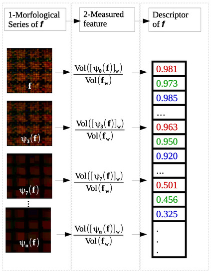
Figure 1.
Steps of feature extraction using mathematic morphology.
- Build a morphological series, which consists of successive morphological filter, , application to image, f.
- Gather values through a measure that allows quantifying the effect of the morphological operator on the image, f.
Most morphological texture descriptors are based on morphological series. The elements in the series are based on properties of the structural element, such as size, shape, and orientation [6,18]. The morphological series is later passed to a feature extraction measure for classification.
3.1. Grayscale Morphological Series
We define a morphological series, , as a series of images, resulting from different applications of a morphological filter, , to the input image, f. The different elements of the series result from the modifications of a property, , of the structuring element, b, such as size. Formally:
where the first element of the series, , is the original image. Different filters, (such as dilation, erosion, opening and closing), together with the characteristics of the structuring element, allow morphological series to extract specific characteristics from the image [19,20].
The Granulometry and Morphologic Covariance will be the morphological series, we will use to extract features from the images. They were proven to be useful techniques for feature extraction in other works [6,16,21].
3.2. Granulometry
We adopt the simplified and normalized notation, , from Aptoula et al. [20], defined as:
where the structuring element, b, is incremented n times. Normalizing the function by the original volume, , allows for size invariance. The volume of an image, f, is defined as:
Figure 2 shows examples of a structuring element which is increased two times.
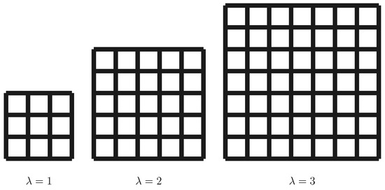
Figure 2.
Structuring elements for granulometry: squares with side .
3.3. Morphological Covariance
Generally speaking, textures can be characterized by the spatial distribution of their patterns. The morphological covariance provides information about periodicity, orientation and rugosity of patterns found in textures through the distribution of orientations and distance of matching pixels [20].
The morphological covariance, K, of an image, f, is defined as the volume of an image after eroding, , the input. The structuring element is composed by two points, . These points are not necessarily adjacent, so their separation can be represented as the vector, . Therefore, the distance and direction between them is, and , respectively.
In practice, we use the normalized morphological covariance defined as:
where represents one of the n combinations of distances and orientations for and , and is the normalization factor. Figure 3 shows examples of variations of a two-point structuring element.
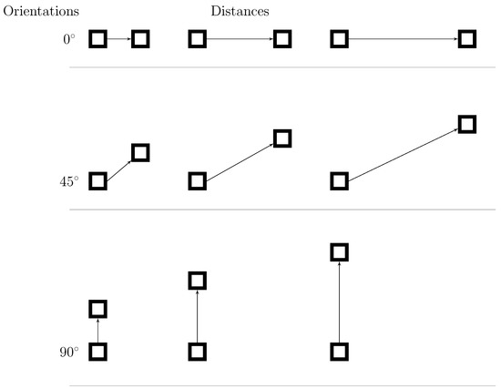
Figure 3.
Structuring elements for morphological covariance: pairs of pixels for different orientation and distances.
3.4. Color Extension for Morphological Series
We use the Lefevre extension for vectorial processing [18]. Formally:
where is a color channel of, .
The application of the vectorial morphological filter, , results in a new color image.
Each channel, , is taken independently in the volume calculation or any other measure that is used in the classification.
Correspondingly, the morphological filter, is applied to each channel independently for marginal processing [18] as:
where is a color plain of .
4. Proposal
We propose the integration of inter-channel measures into color texture descriptors based on morphological series. The initial texture descriptor is the normalized volume of color channel for each element in the morphological series [9,18]. Extending the descriptor with inter-channel measures allows the characterization of the correlation between the color plains.
The correlation between the color plains means that if the intensity changes, all three components will change. This is one of the properties that characterize the RGB space in applications involving a natural color image [22]. Figure 4a,b show the normalized volume descriptors of a sample RGB texture. In both cases, the volume of a channel is normalized by the channel’s volume in the original image. These values do not explicitly reflect the high correlation among the channels, but the residual intensities of the filtered image, .
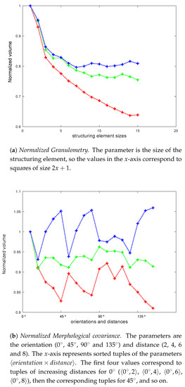
Figure 4.
Color channel comparison of the normalized volume of morphological series for sample 000242 (OutexTC00013). The y-axis represents the normalized volume of the channel and the x-axis represents the different parameters used to calculate the volume. The color of the line indicates the corresponding color channel.
Analogously, Figure 5a,b show the raw volume descriptors of the sample. In theses images, the correlation between the different color channels can be noticed, as the volumes change simultaneously. However, some normalization is required.
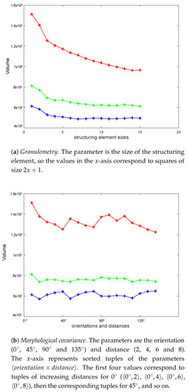
Figure 5.
Color channel comparison of the raw volume of morphological series for sample 000242 (OutexTC00013). The y-axis represents the raw volume of the channel and the x-axis represents the different parameters used to calculate the volume. The color of the line indicates the corresponding color channel.
While intra-channel measures collect and process information from each channel independently, inter-channel measures work with information of multiple channels. Previous works have shown some benefits of the usage of inter-channel measures for texture descriptors using co-occurrence matrices [23,24]. Co-occurrence matrices are two-dimensional histograms of intensity levels for pairs of color channels [23,25].
Our proposal is to use texture descriptors that join the normalized volume of the morphological series and an inter-channel measure:
The volume is used as an intra-channel measure, which will complement the information retrieved by the inter-channel measure.
We compare our proposal to descriptors that use either intra-channel measures or inter-channel measures alone, and descriptors that join volume and intra-channel measures.
4.1. Characterization/Intra-Channel Measures
Previous work has shown that characterization measures that do not use spatial information obtain similar results as texture descriptors compared to ones that use spatial information [6]. Most of these measures are defined for monochromatic images—i.e., they fit the model of intra-channel measures. Therefore, we concatenate the values returned of each color channel in to produce a color texture descriptor.
The following measures have shown good performance as texture descriptors [6].
4.1.1. Variance
The variance of an image, f, characterizes the divergence of pixel intensities. Formally:
where is the number of pixels in f, and is the mean of .
4.1.2. Energy
The energy of an image, f, characterizes the potential of the intensities (loosely seen as frequencies) of the pixels. Formally:
4.1.3. Entropy
The entropy of the histogram, h, for an image, f, is defined as:
where k is the amount of bits encoding the intensity level of a color channel, and h is divided in buckets according to the intensity levels.
4.1.4. Hypervolume
The hypervolume of an image, f, with c color channels is the average volume of -dimensional bounding boxes for pixel intensities [8]. Formally:
where , , are the R, G, and B color channels of f.
4.2. Inter-Channel Measures
Although the measures presented in this section are not novel in themselves, we propose their usage for texture descriptors. To ease notation, we denote hereafter each color plain of a filtered color image, , as , and (Figure 6).
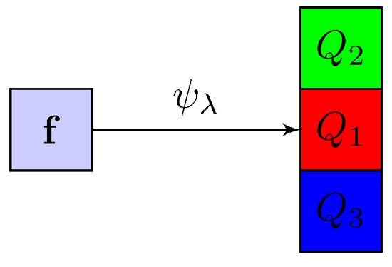
Figure 6.
The morphological filter, , yields images in separate color channels, , and , as output.
First, we present measures based on vectorial distances, which establish how far apart are two elements in vectorial space. Distance-based measures approximate zero as the compared elements increase similarity, and grow when elements decrease similarity. Then, we present proportional measures, which approximate when elements become more similar, and grow or decrease when they become less similar. Finally, we present a histogram-based measure, which retrieves a simple vector as output. The elements of the output vector provide values that express relations between channels of the input image.
4.2.1. Normalized Euclidean Distance
We propose that the euclidean distance between two images, and (which belong to the same element of the morphological series), as the euclidean distance between their volumes.
However, we require to normalize the measure to make it adimensional and independent from size.
Dividing the difference by the standard deviation of all three volumes, , renders the normalized euclidean distance:
The inter-channel descriptor based on this measure is:
4.2.2. Canberra Distance
The Canberra distance is a normalization of the L1 norm of a difference. We establish the Canberra distance of images, and , as:
This distance is subject to —i.e., at least one of the images must have a non-zero volume. Please note that the range of is restricted to the interval.
When , a channel dominates the expression and the distance is maximum.
The inter-channel descriptor based on this measure is:
4.2.3. Inter-Channel Proportion
Another way of establishing the relation between pairs of color channels is by their quotient. Analogous to the previous definitions, we compare images, and , through their volume as:
The quotient provides a simple normalization procedure, which is also size independent. When the channels are very similar, . However, the measure diverges from 1 when the channels are different. In particular, as is more intense than , and as is more intense than .
The inter-channel descriptor based on this measure is:
4.2.4. RG-Volume
The RG-Histogram describes the proportional intensity of each color channel and is normalized by the total intensity, [26]. The original formulation is given by:
We transform Equation (25) to an image histogram, using the channel volume as the intensity indicator. This formulation allows size invariant expressions to compare channels.
Therefore, our formulation of the normalized volume for image is:
Since the relative intensities, , one can be omitted from the inter-channel descriptor as it is linearly dependent on the other two.
Finally the inter-channel descriptor for this measure , based on the red and green channels, is:
5. Experiments
Classification experiments were performed on the OutexTC00013, for general purpose color texture classification, and OutexTC00014 database, for illumination invariance testing [27]. The OutexTC00013 contains 68 textures classes obtained by acquiring a 100 dpi image of size 746 × 538 pixels illuminated by a 2856 K incandescent CIE A light source, each class was divided into 20 non-overlapping sub-images of size 128 × 128 pixels, totaling 1360 texture images (Figure 7).
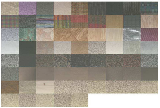
Figure 7.
Textures surfaces in OutexTC00013.
The training set comprises the half of images for each class, totaling 680 images for training and test respectively.
The OutexTC00014 includes OutexTC00013 as the training set. The test set contains the same 68 textures acquired under the two illumination sources. The illumination sources used are 2300 K horizon sunlight (Hor) and a 4000 K fluorescent (TL84). For each illumination source, 1360 images are available, making a total of 2720 test images.
Featured vectors are obtained through granulometry and Morphological Covariance.
For granulometry, square-shaped structuring elements and side pixels were used, varying the size parameter, , from 1 to 15. Small size increments lead better discrimination results [28].
The morphological covariance requires direction and length variations among structuring element pixels. We use the four basic and important directions (, , , ) [12] and lengths from 1 to 20 pixels.
The classifier used is K-nn (K-nearest neighbors) with and euclidean distance. The classification accuracy is computed as the number of successful classifications divided by the total of number of subjects.
We have implemented the morphological filters using ImageJ version 1.52, and performed the classification using Weka version 3.8.3.
5.1. Experimental Results for the OutexTC00013
We performed classification on the OutexTC00013 to compare intra-channel and inter-channel measures with morphological filters applied in vectorial and marginal version. Recall that the erosion (Equation (1)) and dilation (Equation (2)) require to find the minimum or maximum pixel within the structuring element. We use the norm of the color vector representing the pixel to order the pixels within the structuring element.
The results are shown in Table 1. Globally, one can remark the positive effect of the concatenations of the inter-channel measure with standard volume compared to only volume used. For covariance, the accuracy increased in ≈ to ≈ using a vectorial filter and ≈ to ≈ in the marginal filter.

Table 1.
Classification rates in % for the textures in OutexTC00013 using vector ordering and marginal processing. The numbers in bold indicate the top 3 results per column.
The granulometry acruracy increased in ≈ to ≈ using a vectorial filter and in the marginal filter by ≈ to ≈.
5.2. Experimental Results for the OutexTC00014
The OutexTC00014 was used to evaluate our propose performance in invariant light problems, and all images were preprocesed with histogram equalizations to each channel, aiming to provide illumination invariance [29]. As in the previous experiment, we use the norm of the color vector representing the pixel to order the pixels.
Table 2 shows best results for standard descriptors compared with inter-channel measures. Energy, volume, and hypervolume exhibit better results. Equalization preprocessing decreases the intensity differences between volumes of channels and, consequently, the inter-channel measures are not relevant features. This can be seen in Figure 8, which shows the granulometric volumes for original sample texture, 000002, and the image with equalization.
Table 2.
Classification rates in % for the textures in OutexTC00014 using vectorial processing.
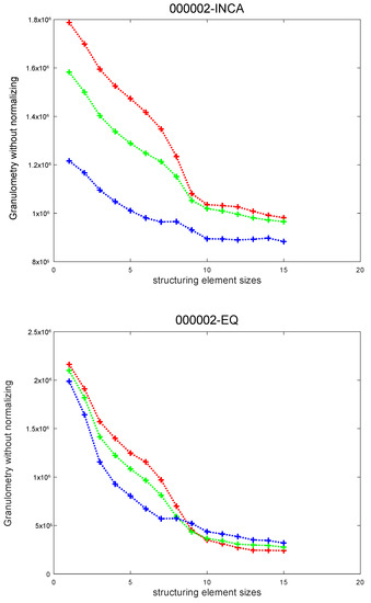
Figure 8.
Comparison of original and equalized raw volumes of morphological series for sample 000002 (OutexTC00014). The y-axis represents the raw volume of the channel and the x-axis represents size of the structuring element. The values in the x-axis correspond to square structuring elements of size . The color of the line indicates the corresponding color channel.
6. Final Discussion and Conclusions
While several inter-channel measures were proposed, there are none that use the mathematical morphology approach. The morphological approach also shows a limited amount of texture descriptors which are dominated by the standard volume. Therefore, in this work we propose a new morphological texture descriptor based on inter-channels measures for RGB color images. The new morphological texture descriptor consists of a standard volume concatenated with inter-channels measures, extracting better features of the underlying image than state-of-the-art morphological texture descriptors.
Our proposal led us to use standard measures, distances, proportions and RG-histograms in a novel application. In particular, coupling the volume with Canberra distance, inter-channel proportion and RG-Volume lead to the best results in the experimental database OutexTC00013, which we suggest for users as the most promising variants of our proposal.
For the experiments on the OutexTC00014, the images were pre-processed with equalization for each channel, thereby exhibiting lower performance in comparison with standard measures.
We believe that future development is likely to come in four ways: adding inter-channel measures, the extending the proposal to other color spaces, employing other types of morphological series and enhancing the performance in the illumination invariance problem. While we have explored the use of some well-known formulas, we are far from an exhaustive analysis. Furthermore, other authors might prefer to develop a custom measure to enhance the proposal. These custom measures would be a likely requirement to extend the proposal to other color spaces, in particular if they are not homogeneous (such as HSL or L*a*b*).
Author Contributions
Conceptualization, N.L.D.S. and J.L.V.N.; methodology N.L.D.S. and J.L.V.N.; software, N.L.D.S.; validation, J.J.C.S.; formal analysis, N.L.D.S., J.L.V.N. and J.J.C.S.; investigation, N.L.D.S.; writing—original draft preparation, N.L.D.S. and J.J.C.S.; writing—review and editing, N.L.D.S., J.L.V.N., J.J.C.S. and M.G.T.; supervision J.L.V.N., M.G.T. and H.L.-A.; project administration, J.L.V.N., M.G.T and H.L.-A.; funding acquisition, M.G.T. and H.L.-A.
Funding
This research was funded by CONACYT, Paraguay, grant number 14-POS-007 and by TIN2015-64776-C3-2-R of the Spanish Ministry of Economic and Competitiveness and the European Regional Development Fund (MINECO/FEDER)
Conflicts of Interest
The authors declare no conflict of interest.
References
- Materka, A.; Strzelecki, M. Texture Analysis Methods—A Review; Technical Report; University of Lodz, Institute of Electronics COST B11 Report: Brussels, Belgium, 1998. [Google Scholar]
- Rao, A.R. A Taxonomy for Texture Description and Identification; Springer Science & Business Media: Berlin/Heidelberg, Germany, 2012. [Google Scholar]
- Rzadca, M. Multivariate Granulometry and Its Application to Texture Segementation. Master’s Thesis, Rochester Institute of Technology, Rochester, NY, USA, 1994. [Google Scholar]
- Tuceryan, M.; Jain, A.K. Texture analysis. In Handbook of Pattern Recognition and Computer Vision; World Scientific Publishing Co.: Singapore, 1993; Volume 2, pp. 235–276. [Google Scholar]
- Elunai, R.T. Particulate Texture Image Analysis with Applications. Ph.D. Thesis, Queensland University of Technology, Brisbane, QLD, Australia, 2011. [Google Scholar]
- Erchan Aptoula, S.L. Morphological texture description of grayscale and color images. Adv. Imaging Electron Phys. 2011, 169, 1–74. [Google Scholar]
- Zhang, J.; Tan, T. Brief review of invariant texture analysis methods. Pattern Recognit. 2002, 35, 735–747. [Google Scholar] [CrossRef]
- Laurențiu, M.; Ivanovici, M. Color and Multispectral Texture Image Analysis–Models, Features and Applications. Learn. Technol. 2015, 25, 287–300. [Google Scholar]
- Angulo, J.; Serra, J. Morphological color size distributions for image classification and retrieval. In Proceedings of the Advanced Concepts for Intelligent Vision Systems, Ghent, Belgium, 9–11 September 2002; pp. 46–53. [Google Scholar]
- Burger, W.; Burge, M.J. Digital Image Processing: An Algorithmic Introduction Using Java; Springer Science & Business Media: Berlin/Heidelberg, Germany, 2009. [Google Scholar]
- Batman, S.; Dougherty, E.R. Size distributions for multivariate morphological granulometries: Texture classification and statistical properties. Opt. Eng. 1997, 36, 1518–1529. [Google Scholar]
- Hanbury, A.; Kandaswamy, U.; Adjeroh, D.A. Illumination-invariant morphological texture classification. In Mathematical Morphology: 40 Years On; Springer: Berlin/Heidelberg, Germany, 2005; pp. 377–386. [Google Scholar]
- Tang, X.; Stewart, W.K.; Vincent, L.; Huang, H.; Marra, M.; Gallager, S.M.; Davis, C.S. Automatic plankton image recognition. In Artificial Intelligence for Biology and Agriculture; Springer: Berlin/Heidelberg, Germany, 1998; pp. 177–199. [Google Scholar]
- Kotsiantis, S.B.; Zaharakis, I.; Pintelas, P. Supervised machine learning: A review of classification techniques. Emerg. Artif. Intell. Appl. Comput. Eng. 2007, 160, 3–24. [Google Scholar]
- Matheron, G.; Serra, J. The birth of mathematical morphology. In Proceedings of the ISMM 2000, Palo Alto, CA, USA, 26–29 June 2000. [Google Scholar]
- Matheron, G. Random Sets and Integral Geometry; John Wiley & Sons: Hoboken, NJ, USA, 1975. [Google Scholar]
- Aptoula, E.; Lefevre, S. A comparative study on multivariate mathematical morphology. Pattern Recognit. 2007, 40, 2914–2929. [Google Scholar] [CrossRef]
- Lefèvre, S. Beyond morphological size distribution. J. Electron. Imaging 2009, 18, 013010. [Google Scholar] [CrossRef]
- Vincent, L. Granulometries and opening trees. Fundam. Inform. 2000, 41, 57–90. [Google Scholar]
- Aptoula, E.; Lefèvre, S. On morphological color texture characterization. In Proceedings of the International Symposium on Mathematical Morphology (ISMM), Montreal, QC, Canada, 21–22 October 2007; pp. 153–164. [Google Scholar]
- Maragos, P. Pattern spectrum and multiscale shape representation. IEEE Trans. Pattern Anal. Mach. Intell. 1989, 11, 701–716. [Google Scholar] [CrossRef]
- Tsagaris, V.; Anastassopoulos, V. Multispectral image fusion for improved rgb representation based on perceptual attributes. Int. J. Remote Sens. 2005, 26, 3241–3254. [Google Scholar] [CrossRef]
- Arvis, V.; Debain, C.; Berducat, M.; Benassi, A. Generalization of the cooccurrence matrix for colour images: Application to colour texture classification. Image Anal. Stereol. 2011, 23, 63–72. [Google Scholar] [CrossRef]
- Martínez, R.; Richard, N.; Fernandez, C. Alternative to colour feature classification using colour contrast ocurrence matrix. In Proceedings of the International Conference on Quality Control by Artificial Vision 2015 International Society for Optics and Photonics, Le Creusot, France, 3–5 June 2015; p. 953405. [Google Scholar]
- Presutti, M. La matriz de co-ocurrencia en la clasificación multiespectral: Tutorial para la enseñanza de medidas texturales en cursos de grado universitario. In Proceedings of the 4ª Jornada de Educação em Sensoriamento Remoto no Âmbito do Mercosul, São Leopoldo, RS, Brazil, 11–13 August 2004. [Google Scholar]
- Van De Sande, K.; Gevers, T.; Snoek, C. Evaluating color descriptors for object and scene recognition. IEEE Trans. Pattern Anal. Mach. Intell. 2010, 32, 1582–1596. [Google Scholar] [CrossRef] [PubMed]
- Ojala, T.; Mäenpää, T.; Pietikainen, M.; Viertola, J.; Kyllönen, J.; Huovinen, S. Outex-new framework for empirical evaluation of texture analysis algorithms. In Proceedings of the 16th International Conference on Pattern Recognition, Quebec City, QC, Canada, 11–15 August 2002; Volume 1, pp. 701–706. [Google Scholar]
- de Ves, E.; Benavent, X.; Ayala, G.; Domingo, J. Selecting the structuring element for morphological texture classification. Pattern Anal. Appl. 2006, 9, 48–57. [Google Scholar] [CrossRef]
- Finlayson, G.; Hordley, S.; Schaefer, G.; Tian, G.Y. Illuminant and device invariant colour using histogram equalisation. Pattern Recognit. 2005, 38, 179–190. [Google Scholar] [CrossRef]
© 2019 by the authors. Licensee MDPI, Basel, Switzerland. This article is an open access article distributed under the terms and conditions of the Creative Commons Attribution (CC BY) license (http://creativecommons.org/licenses/by/4.0/).