Abstract
In this paper, a high precision detection method of salient objects is presented based on deep convolutional networks with proper combinations of shallow and deep connections. In order to achieve better performance in the extraction of deep semantic features of salient objects, based on a symmetric encoder and decoder architecture, an upgrade of backbone networks is carried out with a transferable model on the ImageNet pre-trained ResNet50. Moreover, by introducing shallow and deep connections on multiple side outputs, feature maps generated from various layers of the deep neural network (DNN) model are well fused so as to describe salient objects from local and global aspects comprehensively. Afterwards, based on a holistically nested edge detector (HED) architecture, multiple fused side outputs with various sizes of receptive fields are integrated to form detection results of salient objects accordingly. A series of experiments and assessments on extensive benchmark datasets demonstrate the dominant performance of our DNN model for the detection of salient objects in accuracy, which has outperformed those of other published works.
1. Introduction
With astonishing ability, humans are able to detect visually distinctive, so-called salient objects/regions effortlessly and rapidly. Benefitting from selective attention mechanisms of human visual systems (HVSs), people capture the most obvious objects from complex scenes and implement analysis and treatment, and this helps to greatly improve the efficiency of information perception [1,2,3].
Different from fixation prediction, the aim of saliency detection lies in locating the most remarkable objects in the scene accompanied with a binary segmentation result output [4,5,6]. In general, these methods can be divided into two categories (i.e., bottom-up and top-down approaches) driven by stimulus and tasks, respectively. Early bottom-up approaches usually adopted hand-designed features or combinations of them. However, limited with the cognition of HVS, the mechanism of feature selection and combinational optimization was unclear. The main disadvantage of hand-designed features mainly lies in its low generalization ability. Some handcraft features are deigned for specific tasks without accounting for variability in the input data. They also suffer from a lack of human expertise. Meanwhile, owing to the application of space pyramid theory in multi-scale analysis, the resolution of saliency map was relatively low, and this caused salient objects to be inaccurately located.
With the breakthrough of deep learning, early methods relying on low-level vision cues have been fast superseded in many fields, including handwritten digit recognition, pedestrian detection, and automatic drive. In the field of saliency detection, deep convolutional networks have also acquired enormous successes [7,8,9]. In the issue of detection for salient objects, the fusion of multi-scale features is very important for achieving good results of saliency maps and has been widely referenced in many published papers [10,11].
Inspired by the achievements of deep semantic segmentation, the inherent hierarchical structure of DNN models is very conducive to the extraction of multi-scale features of salient objects [12,13]. In Figure 1, it can be seen that saliency maps generated from deep side outputs of DNN models mainly focus on global appearances of the object. As a contrast, saliency maps generated from shallow side outputs capture detailed information such as textures and skeletons. Both of them are necessary for achieving the high precision detection of salient objects [14,15].
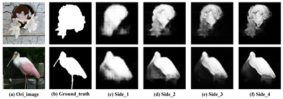
Figure 1.
Saliency maps generated from various side outputs.
In this paper, with proper combinations of shallow and deep connections on various side outputs generated from different layers, a high precision detection method of salient objects based on a symmetric end-to-end DNN model is proposed. Generally, improvements of our method mainly focus on four aspects:
(1) A symmetric end-to-end architecture with stronger backbone networks.
An end-to-end encoder and decoder DNN architecture is proposed in this paper. Moreover, an ImageNet pre-trained ResNet50 is adopted instead of VGG16 to improve the ability of feature extraction for backbone networks [16].
(2) Resolution recovering based on nonlinear transposed convolution.
The nonlinear transposed convolution adopted in our model helps to recover the resolution of feature maps with higher accuracy, and this works toward outperforming the bilinear interpolation applied in fully convolutional networks (FCNs) [17].
(3) Combinations of shallow and deep connections on various side outputs.
Combinations of shallow and deep connections on various side outputs help to integrate feature maps with different sizes of receptive fields. Such integration of overall and detailed information has been validated to be very helpful to achieve a higher accuracy detection of salient objects [18,19].
(4) HED-based architecture with the fusion of multiple side outputs.
Outputs generated from various layers of DNN models focus on different scale information of salient objects. Inspired by HED architecture, multiple side outputs are well fused to integrate multi-scale information that helps to promote accuracy further [20].
2. Related Work
During the past two decades, an extremely rich set of detection methods of salient objects has been well developed. Conventional detection methods of salient objects are primarily based on hand-crafted local features, global features, or the combination of them. A complete review is beyond the scope of this paper, and details can be acquired from a recent survey paper published by Borji A. et al. [21]. In this paper, we mainly focus on developments of deep leaning based detection methods of salient objects.
The inherent hierarchical architecture of DNN models is conducive to the extraction of feature maps with various scale information, which is vital for the high precision detection of salient objects. The literature published by Li G. et al. demonstrates an early attempt [22]. In their work, multi-scale information was acquired by manually selected local images centered by salient objects such that their corresponding generalization abilities are limited. The method of SALICON [23] published by Huang X. et al. in ICCV2015 puts forward another effective solution. In their method, sub-sampled and full resolution images were fed into DNN models (e.g., AlexNet [24]). Then, generated coarse and fine feature maps were concatenated and interpolated to produce a saliency map. Cornia M. et al. proposed a multi-level neural network for the detection of salient objects in ICPR2016 [25]. In their work, with a feature encoding network, feature maps extracted from different layers of an end-to-end DNN model were well combined. They also proposed a new loss function to tackle the imbalance problem of saliency maps. Such a highly efficient end-to-end framework has also been applied in many other outstanding saliency detection models. Inspired by HED [20], Hou Q. et al. proposed a deeply supervised salient object detection model by introducing short connections on skip layers in CVPR2017 [26]. Different from previous methods, hierarchical side outputs produced from various layers were fused to form one integrated saliency map, and this helped to capture the multi-scale information of the target. Similarly, Wang W. et al. proposed a deep visual attention prediction model in TIP2018 [27]. In their work, dense connections between skip layers were discarded from the organization structure of the reference [26] so as to simplify the network architecture at the expense of some performance degradation. The motivation and impacts are worth discussing further.
With the similar task of object segmentation, achievements of deep semantic segmentation can be referenced for the high precision detection of salient objects. The FCN proposed by Long J. et al. in CVPR2015 replaced the full connection layer with convolutional layers, and this provides the FCN with the ability to deal with arbitrary sizes of input images [28]. As a strong baseline method, the FCN has been applied in a wide range of applications, including Mask-RCNN [29]. However, the bilinear interpolation for resolution-retrieving of extracted feature maps is the main shortcoming of FCN. The reason for this lies in the fact that such operation ruins the original spatial relationship between image pixels. In order to solve this problem, Badrinarayanan V. et al. proposed a deep fully convolutional neural network for semantic pixel-wise segmentation termed SegNet in PAMI2017 [30]. The innovation of SegNet lies in its encoder–decoder architecture. The nonlinear resolution-recovering through transposed convolution in the decoder part of SegNet overcomes the mode of bilinear interpolation adopted by the FCN with higher accuracy. However, the encoder–decoder architecture applied by SegNet is inclined to fall into over-fitting, even with rich training samples. For better performance, Ronneberger O. et al. proposed a novel convolutional network for biomedical image segmentation called U-Net [31]. The unique skip-layer architecture concatenates shallow and deep layers symmetrically, and this is conducive to the propagation of gradient information in DNN models [32]. Zhao H. S. et al. proposed another effective model for the fusion of multi-scale information called PSPNet [33]. With pyramid pooling and the integration of feature maps with various scales, PSPNet can both extract large and/or small objects with higher accuracy.
Based on convolutional neural networks (CNNs), the idea of feature clustering has also been widely applied in recent works of object detection and recognition. A recurrent convolutional neural network (RCNN)-based visual odometry approach for endoscopic capsule robots was proposed by Turan M. et al. in [34]. On the one side, just-in-moment features were well extracted by CNNs. On the other side, by means of the RCNN, inference of dynamics across the frames could also be well obtained. Through the fusion of these two powerful deep-learning-based models, an outstanding monocular visual odometry method with high translational and rotational accuracies was achieved. The clustered features can also be used in intelligent systems for disease diagnosis. Połap D. et al. proposed a smart home system to diagnose skin diseases for residents in the house [35]. With the aid of a SIFT algorithm and a histogram comparison, clusters of potential areas were first located. These cluster images were then put forward into CNNs to find real disease areas. With the aid of CNNs, Babaee M. et al. proposed a novel background subtraction method from video sequences [36]. In their method, input frames along with the corresponding background images were patch-wise processed. These fused image patch stacks contained mixed information regarding the foreground and the background. Therefore, the segmentation results could take comprehensive consideration of the detection scene so as to generate high accuracy segmentation results. The idea of feature clustering can also be used in model optimization. A multi-threading mechanism to minimize training time by rejecting unnecessary weight selection was proposed by Połap D. et al. in [37]. The multi-core solution was utilized to select the best weights from all parallel trained networks. A systematic investigation of the impact of class imbalance on classification performance of convolutional neural networks (CNNs) was proposed by Buda M. et al. in [38]. Frequently used methods including oversampling, undersampling, two-phase training, and thresholding were compared, and the optimal solution against class imbalance for deep learning was summarized. An unsupervised extraction of low or intermediate complexity visual features with spiking neural networks (SNNs) was proposed by Kheradpisheh S. R. et al. in [39]. They introduced the technology of spike-timing-dependent plasticity (STDP) into a DNN and presented a temporal coding scheme to selectively fire neurons according to intensities of activation. With the combination of STDP and latency coding, the manner in which primate visual systems learn was well explored.
Based on reviews of related literature, connection mechanisms of various types of DNN models are deeply discussed in Section 3. Through comparative analysis of their merits and drawbacks, a kind of scheme for combinatorial optimization of shallow and deep connections will be put forward accordingly.
3. Analysis and Optimization of the Connection Mechanism of DNNs
As mentioned above, existing DNN models for the detection of salient objects can be summarized into two typical architectures, i.e., the FCN-type architecture and the encoder–decoder type architecture. In this section, based on the analysis of various DNN model structures, a series of improvements will be carried out to generate the framework of our proposed DNN architecture.
3.1. Fully Convolutional Networks (FCNs)
FCNs have been adopted in many strong detection algorithms of salient objects (e.g., [26,27]). Based on comparisons of backbone networks architectures, configurations of existing FCN-net-based saliency detection DNN models can be classified into three categories: (1) a single stream with a single output; (2) multi-streams with a single output; (3) a single stream with multiple side outputs. Model structures of various types of FCNs are shown in Figure 2.
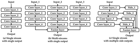
Figure 2.
Various types of fully convolutional network (FCN) architectures.
(1) A single stream with a single output.
Figure 2a shows FCNs based on a single-steam backbone network. With the aid of convolutional layers, semantic features are extracted from original input images. Afterwards, the method of bilinear interpolation is applied onto extracted feature maps, and locations of salient objects are achieved as a result. A fully convolutional architecture of FCNs makes the network capable of dealing with arbitrary sizes of input images. Meanwhile, shared parameters between convolutional kernels are also helpful to improve the efficiency of the network.
(2) Multi-streams with a single output.
Based on initial explorations of detection algorithms for salient objects, DNN models with multi-stream architecture shown in Figure 2b have been widely applied. With the aid of pyramid spatial transformation, multi-scale information is extracted from original input images with various sizes [40]. This approach has also been referenced by authors using traditional methods [41].
(3) A single stream with multiple side outputs.
The third architecture of FCNs exhibited in Figure 2c is inspired by HED architecture. The main difference between Figure 2a,c is that the former one only exports a single prediction from the network. As a contrast, the latter generates multi-level predictions from various hidden layers of the backbone network. With supervisions directly propagated back to the hidden layers, this architecture helps networks quickly converge to a global optimal solution. Moreover, it can be regarded as a lightweight version of multi-stream FCNs shown in Figure 2b, and the quantity of parameters can be well controlled accordingly.
As a strong baseline architecture, FCNs still face drawbacks that need to be overcome. Spatial information among pixels in input images is lost during the operation of max- pooling and/or convolution with various strides. In addition, backbone networks can be strengthened further to enhance the ability of feature extraction to help better locate salient objects with higher accuracy [42].
3.2. Deep Convolutional Encoder–Decoder Networks (EN-DE Nets)
In order to overcome the drawbacks of FCNs, deep convolutional encoder–decoder networks (EN-DE nets) have seen many improvements in terms of model structure. Like FCNs, the architecture of EN-DE nets can be divided into three categories: (1) single-stream EN-DE nets; (2) EN-DE nets with a skip-layer architecture; (3) EN-DE nets with multiple side outputs. These structures are shown in Figure 3.
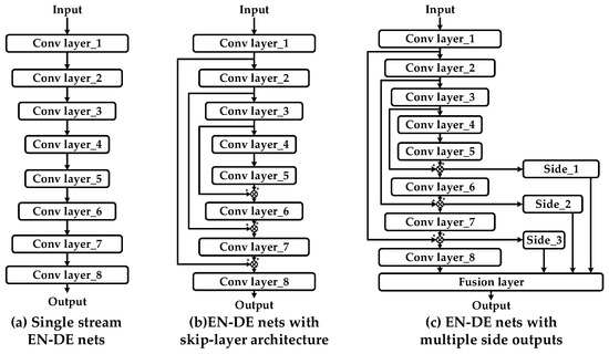
Figure 3.
Various types of encoder–decoder network (EN-DE net) architectures.
(1) Single-stream EN-DE nets.
The architecture of EN-DE nets with single stream backbone networks exhibited in Figure 3a can be separated into two symmetric parts. The former, called “encoder”, is in charge of feature extraction, and the latter, termed “decoder”, is responsible for resolution reconstruction of feature maps correspondingly. The loss between the prediction and the ground truth is back-propagated to adjust the weights of hidden neurons. However, once the outputs of neurons in the shallow layers fall into insensitive regions of the activation function, gradient information cannot be effectively transmitted to deeper layers. With increasing layers, such a single stream architecture tends to become trapped into over-fitting. The detailed reason for this phenomenon has been illustrated in [16].
(2) EN-DE nets with a skip-layer architecture.
Inspired by bottleneck layers adopted in the residual module, EN-DE nets with a skip layer architecture (e.g., U-Nets) help to propagate the flow of information and prevent the model from over-fitting. Meanwhile, feature maps extracted from shallow layers with a smaller receptive field focus on the details of an object. As a contrast, maps extracted from deep layers with a larger receptive field focus on global views. With the aid of the skip-layer architecture, feature maps with various sizes of receptive field are well fused, and this is beneficial for achieving a higher precision detection of salient objects.
(3) EN-DE nets with multiple side outputs.
Compared with Figure 3b, the architecture shown in Figure 3c integrates multiple side outputs with various sizes of receptive field and has already been applied, e.g., [43]. Meanwhile, this multi-level output architecture also exhibits outstanding performance in the task of object detection (e.g., feature pyramid networks (FPNs) [44]). Based on the fusion of multi-scale feature maps, further modifications of Figure 3c will be discussed in Section 3.3.
3.3. Deep Convolutional Models with Combinations of Shallow and Deep Connections
A multi-level side output architecture helps to integrate attention information from different layers of DNN models, and this is beneficial for achieving more accurate detection of variously sized salient objects [13,25]. In this section, through an analysis of metrics and drawbacks of deep networks with combinations of short connections based on an FCN architecture, our framework of a deep network with combinations of shallow and deep connections based on an EN-DE architecture is put forward accordingly and integrated with improvements of multiple aspects.
(1) A deep network with combinations of short connections based on an FCN architecture.
The model shown in Figure 4 was first published in [26] as an improvement of that shown in Figure 1c. The author also drew comparisons of various short connection patterns, and the model shown in Figure 4 outperformed the compared architectures in terms of accuracy. Intuitively, the main difference between these two models shown in Figure 4 and Figure 1c lies in the addition of short connections between outputs generated from various layers of backbone networks. With the aid of this new model, global and local information of salient objects can be well fused, and higher accuracy segmentation results are achieved as a consequence. Although it overcomes many state-of-the-art DNN models, relying on the comparison of FCNs and EN-DE nets stated above, a series of improvements can be adopted with respect to this structure to propose our DNN model afterwards.
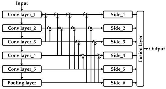
Figure 4.
A deep network with combinations of short connections on FCN architecture.
(2) A deep network with combinations of shallow and deep connections on an EN-DE architecture.
Based on architectures of HED and densely connected convolutional networks [45], our adopted network architecture in this paper, i.e., a deep network with combinations of shallow and deep connections based on an EN-DE architecture, is exhibited in Figure 5. Three main advantages are integrated into this DNN architecture. First, backbone networks based on EN-DE nets with a skip-layer architecture help the model converge faster and better [32]. Meanwhile, nonlinear resolution reconstruction based on symmetric EN-DE nets can also help recover the context information of pixels with higher accuracy. Second, the integration of multi-level side outputs generated from different layers helps to integrate the multi-scale saliency information. Third, shallow and deep connections on various side outputs help to fuse the global and local information of salient objects. Along with the advantages stated above, the details of this architecture will be discussed in Section 4.
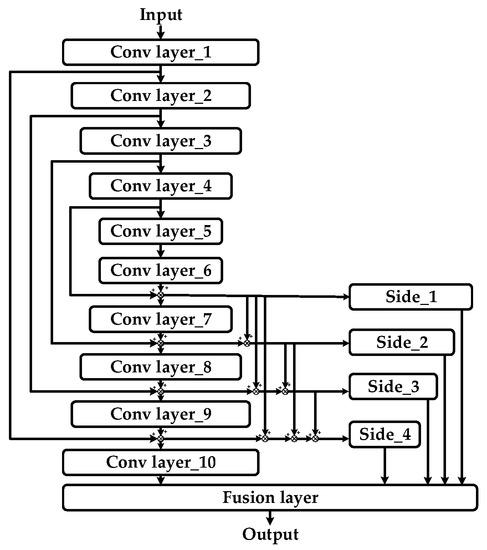
Figure 5.
A deep network with combinations of shallow and deep connections on EN-DE architecture.
4. Saliency Detection Based on a DNN with Combinations of Shallow and Deep Connections
Based on comparisons mentioned above, details of the model structure and its corresponding settings of deep network parameters with combinations of shallow and deep connections are put forward here. Afterwards, the inference process of our proposed detection model for salient objects is discussed in depth. By means of cross-validation, the generalization ability of the model is comprehensively assessed. Finally, with the aid of ablation analysis, contributions of each key module with respect to overall performance improvements are evaluated to validate the rationality of our model design.
4.1. DNN Structures with Combinations of Shallow and Deep Connections for Saliency Detection
The inherent hierarchical structure of DNN models helps to extract the primitive and advanced semantic information of salient objects. Such low and high level features are shown to be both important and complementary in estimating visual attention, and this motivates us to incorporate shallow and deep information for inferring visual attention [46]. The architecture of our proposed deep network with combinatorial optimization of shallow and deep connections is shown in Figure 6, and the whole organization can be divided into four main parts: (1) backbone networks consisting of (1)–(10); (2) skip-layer architectures including four skip-layers of (11)–(18), (12)–(17), (13)–(16), and (14)–(15); (3) multiple side outputs shown as (19)–(22); and (4) shallow and deep connections on various side outputs shown as (23)–(25). The fusion layer is shown as (26).
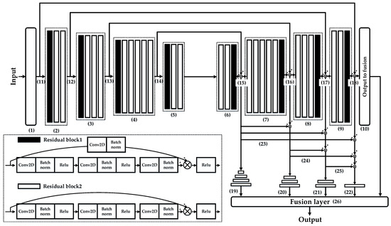
Figure 6.
DNN model structure with combinations of shallow and deep connections.
4.1.1. Backbone Networks
The backbone of the deep network with combinations of shallow and deep connections includes (1) to (10) shown in Figure 6. Intuitively, our model is designed with an end-to-end symmetric mode, and the fully convolutional architecture is very helpful for the promotion of efficiency as a consequence [47].
Meanwhile, we also adopted the technique of transfer learning to help promote the performance of backbone networks in feature extraction. Specifically, the encoder part of the deep network with combinations of shallow and deep connections was upgraded with the ImageNet pre-trained ResNet50 without fully connected layers, and specific implementations are shown in Figure 7. We did not train the networks from scratch but directly invoked pre-trained weight coefficients that achieve 5.25% in top-5 error rates in the ImageNet dataset. The encoder part with pre-trained weight coefficients helps to better extract deep semantic features of salient objects [48]. On the contrary, weights of the decoder part were randomly initialized and adjusted in the process of training. The performance assessment of this transferable model is analyzed in depth in Section 4.2.
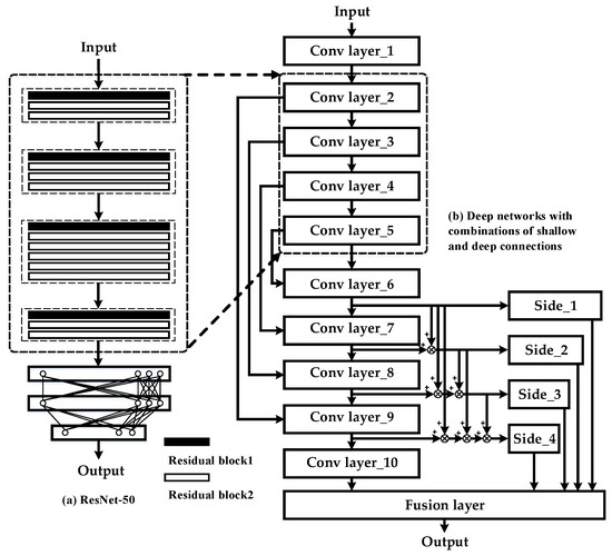
Figure 7.
Transferable DNN model with combinations of shallow and deep connections.
4.1.2. Skip-Layer Architecture
The function of skip layer architectures shown as (11)–(18), (12)–(17), (13)–(16), and (14)–(15) in Figure 6 lies in the integration of feature maps extracted from various layers of backbone networks with different depths. The other important role of skip-layer architectures is to prevent the model from falling into over-fitting. Even if outputs of neurons in the shallow layers fall into insensitive regions of the activation function, with the aid of skip layers, gradient information can still be effectively transmitted to the deeper layers of the network. Further, with the aid of ablation analysis in Section 4.3.4, the effectiveness of such an architecture is analyzed in depth. The details of the connection and the parameter settings of skip-layer architectures are exhibited in Figure 8.
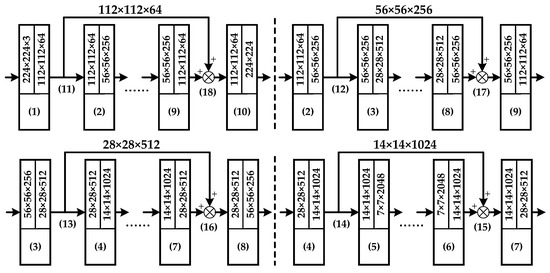
Figure 8.
Structure of skip-layer architectures.
4.1.3. Integrations of Multiple Side Outputs
Based on the HED architecture, the structure of multi-level side outputs is shown in Figure 9. The structure of multi-level side outputs corresponds to modules of (19)–(22) in Figure 6. Outputs generated from deeper layers are better at describing the global characteristics of objects, while those produced by shallower layers tend to represent details that can be clearly seen in Figure 1 [49]. Compared with traditional detection models for salient objects which generate only one saliency map result, the deep network with combinations of shallow and deep layers integrates multi-level side outputs generated from various layers of the decoder part. The inference process will be discussed in Section 4.2.
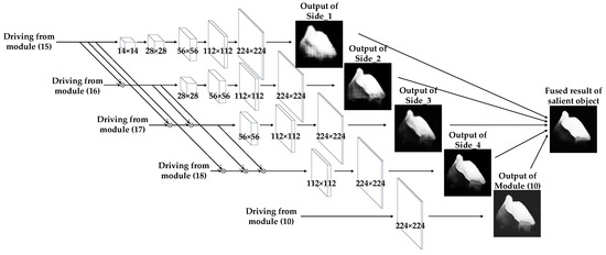
Figure 9.
Structure of multiple side outputs.
4.1.4. Combinatorial Optimization of Shallow and Deep Connections on Various Side Outputs
It has been illustrated that side outputs generated from various layers of DNN models focus on different scale information of salient objects. Based on this phenomenon, shallow and deep connections are constructed to establish contacts of various side outputs to capture the most visually distinctive objects.
In fact, “combinatorial optimization” has two meanings. First, “combination” means that there are many combinatorial modes of these shallow and deep connections between various side outputs. In fact, there are six combinatorial modes in total. Figure 6 only exhibits one of them. All six combinatorial modes of shallow and deep connections are shown in Figure 10.
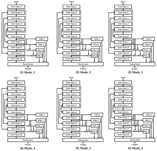
Figure 10.
Various combinatorial modes of shallow and deep connections between different side outputs.
Second, the word “optimization” implies that we should find the best connection mode of shallow and deep connections from models shown in Figure 10. In order to achieve that goal, we trained these models on the ECSSD dataset, and the performance evolution curves are shown in Figure 11.
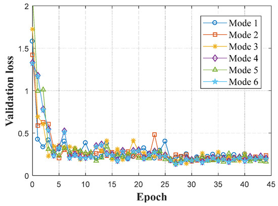
Figure 11.
The performance evolution based on various modes of shallow and deep connections.
In order to make quantitative comparisons, performance indices including validation accuracy, validation loss, and are adopted. The metric of validation accuracy measures the extent to which predicted saliency maps match ground truth masks. In addition, the binary cross entropy L is applied to calculate the metric of validation loss, where . stands for the value of the i-th pixel in the predicted saliency map, and stands for the value of the i-th pixel in the ground truth mask. Moreover, it is necessary to employ the index of the harmonic mean of precision and recall (i.e., ) to evaluate the performance. It is defined as follows:
where , and . S stands for the binary saliency map, and Z stands for the ground truth mask. Generally, the binary saliency map is generated with a threshold that is selected as two times the average gray value of all pixels. Referenced by previous literature [21,26], is selected to be 0.3 to emphasize the importance of precision. Quantitative experimental results are shown in Table 1.

Table 1.
Various combination modes of shallow and deep connections.
From Table 1, it can be seen that exhibits the best performance among the compared DNN models with different combinatorial modes of shallow and deep connections. This is the reason why it is selected to be the optimal DNN model structure. Details about the combinations of shallow and deep connections on various side outputs in are shown in Figure 12.
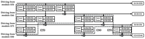
Figure 12.
Structure of shallow and deep connections on various side outputs.
In order to integrate various sizes of feature maps, the operation of transposed convolution is applied to reconstruct the image resolution. Compared with the bilinear interpolation adopted in FCNs, nonlinear transposed convolution can obtain higher accuracy [17]. Performance assessments on shallow and deep connection architecture will be evaluated with ablation analysis in Section 4.3.
4.2. A Saliency Detection Model Based on a DNN with Combinations of Shallow and Deep Connections
Different from previous published approaches, a DNN with combinations of shallow and deep connections integrates multi-level side outputs to generate the saliency map with the structure shown in Figure 9. Here, the inference process of our proposed detection model of salient objects will be discussed.
Assume there are M side outputs generated from backbone networks. Each of them is associated with a classifier with weights represented by Equation (2):
For each branch of side outputs, with the aid of transposed convolution, the resolution of generated feature maps is recovered to be the same size with input images. Then, based on normalized predictions and ground truth saliency maps, pixel-level cross entropy is calculated with Formula (3):
where denotes the cross entropy loss of the k-th side outputs, denotes the pixel at location j of image X, stands for the ground truth saliency map, denotes the collection of all standard parameters of deep networks with combinatorial optimization of shallow and deep connections, and denotes the probability of the activation value at location j. Thus, the objective loss function of side outputs can be represented by Equation (4):
where is the weight of the k-th side loss.
In Figure 6, it can be seen that a weighted-fusion layer is added to connect each side activation. The loss function of this weighted-fusion layer can be represented by Equation (5):
where denotes the fusion weight, denotes the k-th normalized side output saliency maps of the fine-tuned deep networks with combinatorial optimization of shallow and deep connections, and represents the function for measuring the distance between the fused saliency map and the ground truth. Therefore, our final loss function of can be described as Equation (6):
Finally, all the parameters can be learned via minimizing Equation (6) by the algorithm of adaptive moment estimation.
4.3. A Transferable Model with Combinations of Shallow and Deep Connections Based on ImageNet Training
In this section, at first, the process of hyperparametric optimization is discussed. Afterwards, through comparisons of DNN models based on various types of backbone networks, the effectiveness of a transferable model of deep networks with combinations of shallow and deep connections is evaluated. Moreover, with the aid of 10-fold cross-validation, the stability and generalization ability of our proposed model is comprehensively validated. Finally, by means of ablation analysis, performance improvements provided by various key modules of our DNN models is assessed in depth. All contrastive experiments are implemented on the ECSSD dataset [50].
4.3.1. Hyperparameters Optimization
Because the algorithm of Adam [51] was utilized to be the optimizer in our DNN model, main hyperparameters included , the learning rate, , the exponential decay rate of the first moment estimate, and , the exponential decay rate of the second moment estimate. Generally, the default setting (i.e., , , and ) can yield relatively good experimental results. However, in order to further improve the performance, with the aid of a randomized grid search, we implemented an experiment of hyperparameter optimization, and details can be found in the following.
In order to avoid over-concentration of sampling and to find the optimal solution, the interval of hyperparameters in a randomized grid search should be confirmed first. Specifically, for the learning rate , uniform random sampling is implemented at intervals of , , and . For the exponential decay rate of the first moment estimate , uniform random sampling is implemented at intervals of , , and . For the exponential decay rate of the second moment estimate , uniform random sampling is implemented at intervals of , , and . Accordingly, one grid of hyperparameters is formed. Afterwards, 20 points are randomly selected from the grid to form different combinations of hyperparameters. In order to exhibit the process of random sampling intuitively, all of these points are shown in Figure 13, and each point stands for one combination of three hyperparameters.
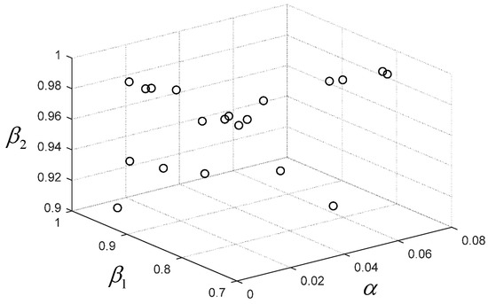
Figure 13.
Random sampling points of hyperparameters.
In order to evaluate the performance, the off-line training was carried out on the DNN model shown in Figure 6 with different combinations of hyperparameters on the ECSSD dataset. Combinations of hyperparameters and their corresponding performance are shown in Table 2. Through a comparison of validation loss, the optimal combination of hyperparameters (i.e., , , and ) was confirmed.
Table 2.
Randomized grid search of hyperparameters and their corresponding performance.
4.3.2. Performance Comparison of Backbone Networks
In Figure 6, it can be seen that the backbone network of our DNN model is designed as a symmetric end-to-end architecture. In order to achieve the goal of high accuracy saliency detection, the method of transfer learning is applied to the backbone network to promote the ability of feature extraction. Specifically, the ImageNet pre-trained ResNet50 without fully connected layers is utilized to be the encoder part. In correspondence, weights of the decoder part are randomly initialized and adjusted during the process of training. In order to comprehensively evaluate improvements generated by the modification of backbone networks, DNN models based on various types of backbone networks are compared with different indices, including Precision–Recall (P-R) curves, accuracy, and loss in the validation dataset. Experimental results are shown in Figure 14.
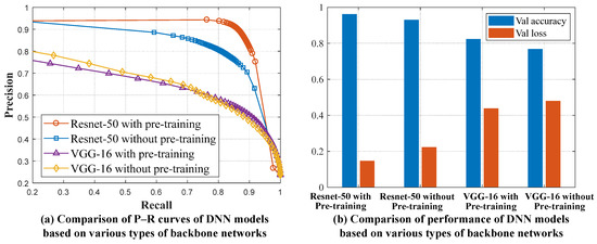
Figure 14.
Performance of various types of transferable DNN models.
All of the compared DNN models are based on the structure shown in Figure 6. The difference mainly lies in the types of backbone networks set to be Resnet50 and VGG16 with/without pre-training, respectively. In order to comprehensively compare the performance of transferable models, P-R curves were drawn based on the whole dataset. Specifically, a series of binary saliency maps were obtained by setting a threshold from 0 to 255 with an increment of 5. By comparing binary saliency maps with their corresponding ground truth masks, pairs of precision and recall scores were counted and averaged among the dataset so as to generate the final P-R curves. Generally, the P-R curves closer to the upper right corner represent a better performance. The P-R curves in Figure 14a show that, with Resnet50 or VGG16, the application of transfer learning improves the detection of salient objects. Moreover, among the compared backbone networks, Resnet50 pre-trained on the ImageNet dataset exhibits remarkable superiorities.
The other direct way to evaluate the performance of DNN models is to monitor the process of performance evolution. During the process of training, after each epoch of iteration, metrics of accuracy and loss will be calculated on the training and validation datasets. In our experiment, once a lower validation loss is achieved, the model will be updated and its corresponding performance indices will be recorded accordingly. The next epoch of training will be then implemented on the model continually. When the process of training is complete, only the best model with the lowest validation loss will be saved. The performance indices of the best model are shown in Table 3. For clarification, results in Table 3 are exhibited in Figure 14b. For the DNN model based on the backbone network of the pre-trained Resnet50, the accuracy of the validation set reached 0.9619 and the loss dropped to 0.1345. Based on this comprehensive analysis, the improvement of backbone networks with transfer learning has been fully validated.
Table 3.
DNN models based on various types of backbone networks.
4.3.3. Cross-Validation and Assessments
In order to evaluate the performance of stability and generalization ability, the method of 10-fold cross-validation was carried out on our DNN model. Specifically, the ECSSD dataset with the capacity of 1000 was divided into 10 sub-samples. Then, nine sub-samples (i.e., 900 image samples) were selected to be the training set and the remaining sub-sample (i.e., 100 image samples) was assigned to be the validation set to test the performance of the DNN model shown in Figure 6 with the backbone of ResNet50. This process was repeated alternately 10 times, and experimental results are shown in Figure 15.
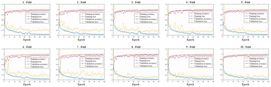
Figure 15.
10-fold cross-validation on the ECSSD dataset.
In Figure 15, it can be seen that the DNN model with the architectures shown in Figure 6 exhibits outstanding performance in terms of accuracy and stability. During 10-fold cross-validation, with different training and validation datasets, our proposed DNN model converges well and achieves a high level of performance accordingly.
Without obvious debasement of the performance, in each fold of cross-validation, the settings of hyperparameters were set to be the same. Specifically, if performance degradation occurred on the (k+1)-th fold of cross-validation, a randomized grid searching of hyperparameters was carried out in the local neighborhood around current optimal parameters. Then the updated hyperparameters were tested on the k-th fold of cross-validation again. If the updated optimal hyperparameters worked well on the k-th fold of cross-validation, they were set as the new solution of optimal hyperparameters. In each fold of cross-validation, only the performance of the best model was recorded. In each fold of cross-validation, all of the images in the dataset were selected to be the training and validation sets. Therefore, the performance of the optimal model was distinct. In order to obtain the mean performance of the model on the whole dataset, all performance indices in each fold of cross-validation were averaged, and the mean value of the performance was achieved accordingly. For a more intuitive exhibition, experimental results in Figure 15 are exhibited in Table 4.
Table 4.
Assessments of 10-fold cross-validation.
From records shown in Table 4, it can be seen that, whether trained by Kth-fold of the dataset or not, our DNN models exhibit a high and stable performance. For the ECSSD dataset, the average accuracy on the validation set was , and the average loss dropped to 0.1345. In each fold, the performance of our DNN model was basically maintained around the average level without obvious fluctuations. Thus, by the method of 10-fold cross-validation, the generalization ability of our proposed DNN models has been fully validated.
4.3.4. Ablation Analysis
Our proposed deep network based on combinations of shallow and deep connections has integrated advantages of multiple key modules. In order to evaluate improvements of each module onto the overall performance, the experiment of ablation analysis was carried out. As stated above, key modules of our DNN model include four main parts, i.e., the symmetric encoder and decoder backbone networks, skip layer architectures, multiple side outputs, and intergrations of side outputs with shallow and deep connections. These key modules are removed step by step from the DNN model to assess the change in performance, and the experimental results are shown in Figure 16.
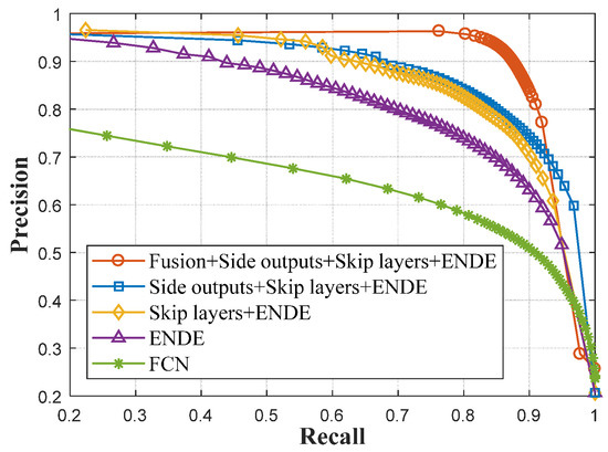
Figure 16.
Performance ablation analysis with Precision–Recall (P-R) curves.
In fact, among these compared models, some of them are very strong baseline methods (e.g., the network based on the encoder and decoder architecture with skip layers refers to U-Net). P-R curves in Figure 16 show that, along with removals of these key modules step by step, the performance of the detection for salient objects was gradually reduced thereupon. Especially, when the fusion of multiple side outputs with shallow and deep connections were removed, the performance dropped obviously by a large margin. This phenomenon validates the importance and effectiveness of the fusion of multiple side outputs with shallow and deep connections proposed in this paper. Meanwhile, the performance of DNN models based on the encoder–decoder architecture generally outperforms that of FCNs, and this is exactly the reason why our model is built up based on such an architecture.
Further, in order to quantitatively demonstrate experimental results, the index of the Intersection over Union (IoU) is evaluated with Equation (6):
where stands for the binary saliency maps processed by threshold segmentation, stands for the ground truth mask images, stands for the pixel number within the area. In our experiment, the adaptive threshold is selected to be twice the average value of the saliency map, and the results of the IoU are shown in Table 5.
Table 5.
Ablation analysis with the Intersection over Union (IoU) score.
Based on IoU scores shown in Table 5, the contribution of each module to overall performance improvements is shown very clearly. The most obvious promotion comes from two aspects, i.e., the encoder–decoder architecture and the fusion of multi-side outputs with shallow and deep connections, which are systematically elaborated in Section 4.1. Compared with existing saliency detection DNN models (most of which are still based on the FCN architecture and/or have no consideration of the fusion of side outputs with various sizes of receptive fields), our proposed network structure shows obvious superiorities.
Corresponding to methods presented in Table 5, binary outputs of saliency maps are exhibited in Figure 17. The effectiveness of our proposed DNN model has thus been fully validated.
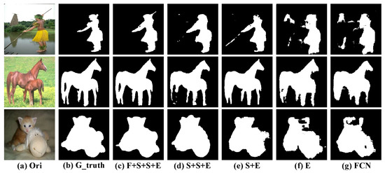
Figure 17.
Performance ablation analysis with binary saliency maps.
4.4. Integrated Architecture of Saliency Detection System
Based on the analysis stated above, details about the architecture of our DNN model and how to find the optimal hyperparameters has been well illustrated. In this section, the integrated architecture of our proposed saliency detection system is provided. The flow chart of the whole system is exhibited in Figure 18.
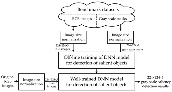
Figure 18.
Integrated architecture of saliency detection system.
In Figure 18, it can be seen that our system can be divided into two main parts. The first part is “off-line training.” For each benchmark dataset, the operation of normalization is implemented onto the original RGB images and their corresponding gray scale ground truth masks. Through image size normalization, all of the images and masks are resized to . Afterwards, based on the resized images and masks, the off-line training is implemented to the DNN model with the architecture shown in Figure 6. The second part is “on-line testing.” Similar to the procedure of training, all of the test images should be first resized to . Then, with the aid of well-trained end to end DNN models, the results of saliency maps with the same size as the inputs are obtained directly without a further need of processing. The performance analysis and assessment of our method for the detection of salient objects is discussed in Section 5.
5. Performance Analysis and Assessment
Through comprehensive analysis, the characteristics of the DNN model based on combinations of shallow and deep connections have been illustrated in depth. In this section, through comparisons with other strong baseline methods, the performance of our DNN model will be synthetically evaluated on extensive saliency detection benchmark datasets. According to experimental results, the metrics and drawbacks of our model will be analyzed, and applicable scenarios will be discussed.
5.1. Benchmark Datasets and Evaluation Indices
5.1.1. Benchmark Datasets
In order to evaluate the performance, comparative experiments were implemented on three widely used saliency detection benchmark datasets: ECSSD [50], MSRA-10K [52], and iCoSeg [53,54].
For the ECSSD dataset, the sizes of the original images and their corresponding masks are exactly the same, mainly , , and . RGB images are stored in the format of jpg. The gray scale mask images are stored in the format of png. The ECSSD dataset has the capacity for 1000 image samples. Moreover, objects in ECSSD usually have a complex appearance, which makes it very suitable for evaluating the description ability of DNN models.
For the MSRA-10K dataset, the sizes of the original images and their corresponding masks are also the same. The range of image size mainly covers , , etc. RGB images are stored in the format of jpg. The gray scale mask images are stored in the format of png. The MSRA-10K dataset has a large quantity of image samples from hundreds of different categories. Most of these images only include one main salient object near the center area.
For the iCoSeg dataset, like ECSSD and MSRA-10K, each RGB image has a corresponding mask with the same size. The image size is mainly , , , or . RGB images are stored in the format of jpg. The gray scale mask images are stored in the format of png. As a small dataset, the amount of image samples in iCoSeg was designed for co-segmentation with only 643 images. Meanwhile, some images in iCoSeg include multiple objects with complex shapes.
According to the design of our proposed DNN model structure, before training images are imported into the DNN model, all of these images and their corresponding masks should be normalized to the size of for all three benchmark datasets. The entire process can also be seen very clearly from the system flow chart shown in Figure 18.
5.1.2. Evaluation Indices
In order to assess the performance, four universally agreed, standard evaluation metrics were adopted: P-R curves, F-measure, intersection-over-union (IoU), and mean absolute error (MAE). Meanwhile, time consumption was also counted to evaluate the efficiency of the compared DNN models. P-R curves, F-measure, and the IoU score are illustrated above, and here we only provide the expression of MAE as follows.
Assuming that the width and height of the original RGB image is , the MAE score can be calculated by Equation (8):
where S stands for the binary saliency map segmented with the threshold of twice the average value, and Z stands for the ground truth correspondingly. MAE is useful in evaluating the applicability of a model, as it reveals the numerical distance between the saliency map and the ground truth.
5.2. Platform and Implementation Details
We constructed the DNN model with combinations of shallow and deep connections on the platform of Keras 2.0.9 using Tensorflow 1.2 as the backend. As mentioned above, the encoder part was designed as an ImageNet pre-trained ResNet50 without fully connected layers. We invoked the weights from the library of Keras instead of training from the scratch. The rest of the model was randomly initialized and adjusted during the procedure of training. All of the weights were adjustable without freezing.
The algorithm of Adam [51] was adopted as the optimizer. During the procedure of training, in order to stably converge to the optimal solution, one adjusting schedule was designed for the learning rate—. Specifically, for the whole 45 epochs training process, in 1 to 30, 31 to 40, and 41 to 45 epochs, learning rates, , were set to be 0.0022, 0.00022, and 0.000022, respectively. The hyperparameters of and remained unchanged throughout the training.
When the process of training was finished, the best model with the minimum loss in the validation set was saved. It took about 2.5, 30, and 2 h to train the model for the ECSSD, MSRA-10K, and iCoSeg datasets, respectively. Two NVIDIA GEFORCE 1070Ti GPUs with 16 GB memory under multi-GPU mode provided the computing power. All experiments were carried out on this platform without further explanations.
5.3. Performance Assessment by Verification on ECSSD
In order to evaluate the performance, five state-of-the-art deep-learning-based saliency detection methods including deep networks with short connections (DSCs) [26], deep visual attention networks (DVAs) [27], networks of static saliency (NSSs) [55], networks of dynamic saliency (NDSs) [55], and deep multi-level networks (DMLNs) [25] were applied to compare with our DNN models. Meanwhile, five conventional saliency detection methods, i.e., RBD [56], DSR [57], MC [58], GR [59], and CA [60] were also employed, and source codes were all obtained from the project website of [21]. First, on the ECSSD dataset, P-R curves of these compared methods were drawn, which can be seen in Figure 19.
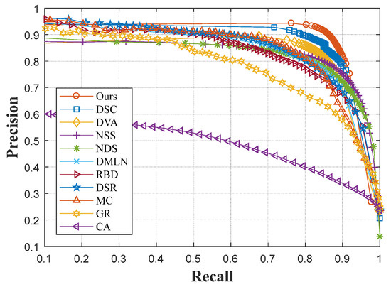
Figure 19.
P-R curves of the ECSSD dataset.
In Figure 19, it can be seen that our model has the best performance. With stronger backbone networks based on an encoder–decoder architecture, our model overcomes the performance of the DSC, which is designed in FCNs. In addition, DVA and DMLN models were also built on the FCN architecture. Meanwhile, in these two models, feature maps with different sizes of receptive fields were merged directly without fusions between each other. Similar situations also occurred with respect to NSS and NDS. Although these two models are based on the encoder–decoder architecture, their single steam models do not consider the utilization of feature maps generated from various layers of the network. Therefore, useful multi-scale information regarding salient objects was discarded, resulting in relatively poor performance.
Extensive indices including precision, recall, F-measure, IoU, and MAE were also adopted to assess the performance between contrastive DNN models. In the process of comparison, continuous saliency maps were first processed by the operation of threshold segmentation. For the sake of fairness, thresholds were all set to be twice the average value of the saliency maps in each saliency detection DNN model. Comparison results are shown in Figure 20.
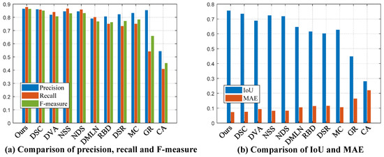
Figure 20.
Various performance indices on the ECSSD dataset.
In Figure 20, it can be seen that our model has obvious advantages, regardless of precision or recall. This is mainly due to the coordination of multiple key modules. With the aid of the fusion of multiple side outputs, our models capture the local and global information of salient objects comprehensively. In addition, the score of the IoU and MAE indicate that our model can accurately locate not only salient objects, and the probability of false alarm is controlled at a low level in irrelevant background areas.
At last, a visual comparison of saliency maps is exhibited in Figure 21. The first column exhibits original RGB images, and the second column exhibits their corresponding binary ground truth masks. The third and later columns stand for continuous saliency maps generated by various contrastive methods. It is obviously noticed that our saliency maps are most similar to the ground truth and highlight the saliency objects with high accuracy.
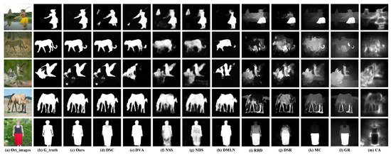
Figure 21.
Saliency maps generated by various methods on the ECSSD dataset.
5.4. Performance Assessment by Verification on MSRA-10K
Similarly, the performance of our proposed detection model of salient objects are also evaluated on the large scale MSRA-10K dataset. Because the generalization ability of our DNN model has been well validated through 10-fold cross-validation in Section 4.3.3, here we randomly selected 6000 samples from the dataset as the training set. The remaining 4000 samples are utilized as the test set to evaluate the performance of well trained DNN models. For the sake of fairness, all models were trained on the same training set. P-R curves are shown in Figure 22.
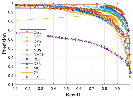
Figure 22.
P-R curves of the MSRA-10K dataset.
In Figure 22, it can be seen that our model still exhibits the best performance. Compared with the ECSSD dataset, objects in MSRA-10K generally have a relatively simple shape. As a consequence, the performance of contrastive DNN models for saliency detection is promoted. Meanwhile, other indices are also compared, and the experimental results are shown in Figure 23.
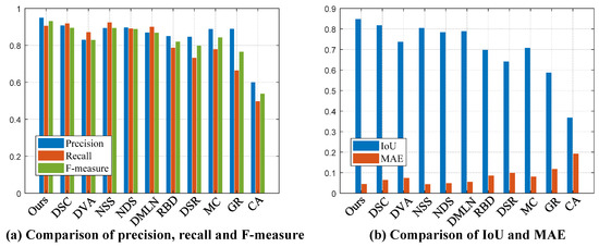
Figure 23.
Various performance indices on the MSRA-10K dataset.
In Figure 23, it can be seen that our detection model of salient objects shows obvious advantages compared with other DNN models. This superiority is mainly due to the design of the network architecture. The coordination of multiple key modules makes our model able to locate the most salient object with high accuracy. In addition, our model also demonstrates a strong ability in terms of recall and other performance indices.
Finally, a visual comparison of saliency maps on the MSRA-10K dataset are provided in Figure 24. Like Figure 21, the first and second columns exhibit original RGB images and their corresponding ground truth masks, respectively. The third and later columns exhibit saliency maps generated by contrastive models. From comparisons of saliency maps generated from various methods, the advantages of our detection model of salient objects can be viewed intuitively.
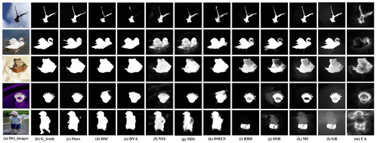
Figure 24.
Saliency maps generated by various methods on the MSRA-10K dataset.
5.5. Performance Assessment by Verification on iCoSeg
Based on a small-scale dataset, we also validated the performance of DNN models on the iCoSeg dataset. Compared with MSRA-10K, the capacity of iCoSeg is too small for training a deep network with a structure shown in Figure 6. However, with the aid of the unique multiple side output architecture, supervisions can be directly propagated back to the hidden layers, which helps the network quickly converge to a global optimal solution. Meanwhile, skip layer architectures can also help the network from falling into over-fitting. Therefore, even with fewer training sets, our model can still perform well. Specifically, from the total 634 image samples, 450 of them were randomly selected as the training set, and the remaining images were utilized to validate the performance of the well trained DNN models. For the sake of fairness, all of the models were trained on the same training set, and the P-R curves are shown in Figure 25.
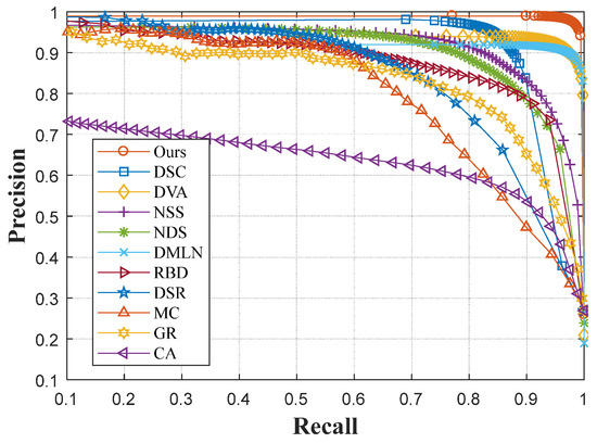
Figure 25.
P-R curves of the iCoSeg dataset.
In Figure 25, it can be seen that the precision of our DNN model dropped sharply only when the value of the recall approached 1. Among most of the other compared methods, the value of the precision dropped gradually with the increase in recall. This phenomenon indicates that the saliency maps generated by our proposed model shows a very high contrast.
Meanwhile, we also compared other performance indices between these contrastive methods. It can be seen in Figure 26 that, from a comprehensive comparison of various indicators, our DNN model exhibits a strong capability compared with other DNN models. An outstanding model structure design leads to a good performance, even under smaller-scale datasets.
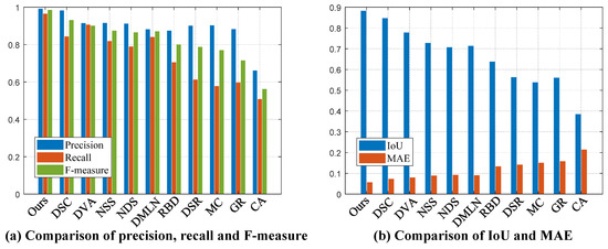
Figure 26.
Various performance indices on the iCoSeg dataset.
For an intuitive visual comparison, saliency maps generated from various DNN models are provided in Figure 27. It can be clearly seen that the saliency maps generated by our model are the most similar with the ground truth masks. The superiority of our model has thus been fully validated.
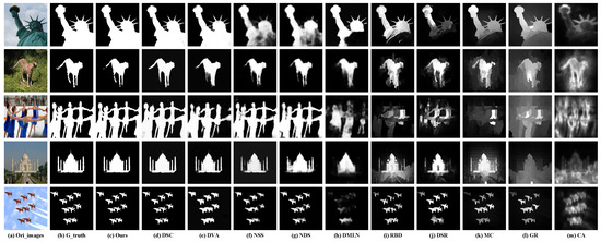
Figure 27.
Saliency maps generated by various methods on the iCoSeg dataset.
In order to further improve the performance of our model on small-scale datasets (e.g., iCoSeg), we also tried to introduce the technique of transfer learning and data augmentation into the process of training. Specifically, we first performed off-line data augmentation to extend the capacity of the original dataset. The operations of data augmentation and some off-line augmented image samples are shown in Figure 28.
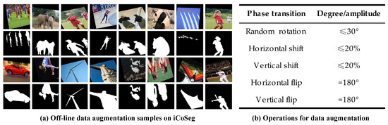
Figure 28.
Off-line data augmentation on the iCoSeg dataset.
For each image, nine corresponding samples were generated, with operations listed in Figure 28b. With the aid of data augmentation, the amount of training sets was expanded to 10 times the original (e.g., 4500 images for the training set of iCoSeg). However, the correlation between these augmented image samples is very high, which is adverse. Thus, we introduced the technique of fine tuning to help further improve the performance. Specifically, weights of the model pre-trained on MSRA-10K were introduced into the new model. Afterwards, this model will continue to be trained on the augmented iCoSeg dataset. In order to evaluate the improvements of performance, evolution curves of validation loss during the process of training are shown in Figure 29.
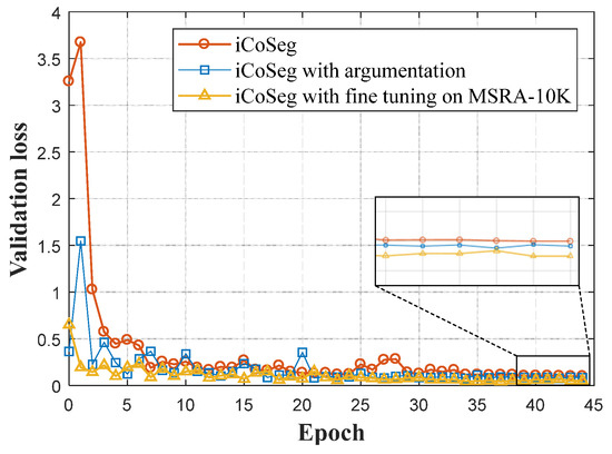
Figure 29.
Performance evolution with data augmentation on the iCoSeg dataset.
In Figure 25, it can be seen that, by means of data argumentation, the performance of our model improves remarkably. Techniques of data augmentation and transfer learning have become necessary approaches to improve the performance of DNN models without the need for special emphasis. The experiment implemented here is only to show that the performance of our model still has room for further improvement. Finally, quantitative experimental results of deep-learning-based saliency detection methods on these benchmark datasets are shown in Table 6.
Table 6.
Performance indices on various benchmark datasets.
From records shown in Table 6, it can be seen that our model shows outstanding performance in accuracy. However, massive adjustable parameters in symmetrical network structure also pulls down efficiency. The original intention of the design of our network is to improve the precision of detection for salient objects. Owing to the update of backbone networks and the introduction of the fusion of multiple side outputs with shallow and deep connections, the number of parameters has increased. This is the reason why our network obviously lags behind FCNs in terms of testing time.
6. Discussion and Comments
The effective extraction of deep features is vital to achieve high accuracy saliency detection. Generally speaking, with deeper backbone networks, the capability of the feature extraction of DNN models is promoted as a consequence. However, with increasing layers and limited training samples, the model tends to become trapped in over-fitting. Skip-layer architectures connecting various depths of DNN models assist the transmission of data flow. Benefitting from this, the performance of DNN models based on encoder and decoder architecture overcomes FCNs by a large margin.
In addition, global and local vision cues are both very important to locate salient objects in complex detection scenes. However, conventional saliency detection methods only utilize the end output of DNN models. The inherent hierarchical structure of DNN models can be used to extract multi-scale feature maps with various sizes of receptive fields. Through the fusion of feature maps extracted from various layers of the DNN model with shallow and deep connections, different scale information of salient objects has been comprehensively utilized. In this way, the detection of salient objects has been significantly improved as a result.
Through comprehensive evaluations on benchmark datasets, experimental results reveal the fact that, with various improvements, our model yields state-of-the-art results in terms of the accuracy of the detection of salient objects. With a series of comparisons, the effectiveness of combinations of shallow and deep connections has also been well validated. In our model, we did not deliberately choose the best network. What we want to emphasize is the idea and approach of how to reinforce the performance of saliency detection through the fusion of multi-scale feature maps on the symmetric encoder and decoder architecture. With the development of research, stronger backbone networks will be put forward continuously. Based on the architecture proposed in this paper, the backbone network can be easily replaced by these stronger networks, and the performance of our model can be further improved accordingly.
7. Conclusions
In order to achieve high precision detection of salient objects, deep convolutional networks with proper combinations of shallow and deep connections are proposed in this paper. With the aid of combinations of shallow and deep connections on multiple side outputs, different scale feature maps are well fused so as to accurately capture the global and local information of salient objects. Benefitting from well designed symmetric end-to-end architecture, a deep network with combinatorial optimization of shallow and deep connections has obvious advantages in detection accuracy, but it still faces the hindrance of low efficiency, and this will be modified in future works.
Author Contributions
The two authors designed the research method and comparative experiments cooperatively. The core idea and overall framework of the article were proposed by S.Q. and L.G. Meanwhile, S.Q. provided very important advices during the process of revision. L.G. implemented experiments, wrote the code and draft. All authors have read and approved the final manuscript.
Funding
This research was funded by the National Nature Science Foundation of China (Grant Nos. 61731001 and U1435220).
Conflicts of Interest
The authors declare no conflict of interest.
References
- Sperling, G. A Brief Overview of Computational Models of Spatial, Temporal, and Feature Visual Attention. In Invariances in Human Information Processing; Routledge: Abingdon, UK, 2018; pp. 143–182. [Google Scholar]
- Liu, T.; Yuan, Z.; Sun, J.; Wang, J.; Zheng, N.; Tang, X.; Shum, H.Y. Learning to detect a salient object. IEEE Trans. Pattern Anal. Mach. Intell. 2011, 33, 353–367. [Google Scholar] [PubMed]
- Borji, A.; Itti, L. State-of-the-art in visual attention modeling. IEEE Trans. Pattern Anal. Mach. Intell. 2013, 35, 185–207. [Google Scholar] [CrossRef] [PubMed]
- Wang, J.; Borji, A.; Kuo, C.C.J.; Itti, L. Learning a combined model of visual saliency for fixation prediction. IEEE Trans. Image Process. 2016, 25, 1566–1579. [Google Scholar] [CrossRef] [PubMed]
- Liu, N.; Han, J.; Liu, T.; Li, X. Learning to predict eye fixations via multi resolution convolutional neural networks. IEEE Trans. Neural Netw. Learn. Syst. 2018, 29, 392–404. [Google Scholar] [CrossRef]
- Xiao, F.; Peng, L.; Fu, L.; Gao, X. Salient object detection based on eye tracking data. Signal Process. 2018, 144, 392–397. [Google Scholar] [CrossRef]
- Ayoub, N.; Gao, Z.; Chen, B.; Jian, M. A synthetic fusion rule for salient region detection under the framework of ds-evidence theory. Symmetry 2018, 10, 183. [Google Scholar] [CrossRef]
- Li, X.; Zhao, L.; Wei, L.; Yang, M.H.; Wu, F.; Zhuang, Y.; Ling, H.; Wang, J. Deep saliency: Multi-task deep neural network model for salient object detection. IEEE Trans. Image Process. 2016, 25, 3919–3930. [Google Scholar] [CrossRef] [PubMed]
- Jiang, H.; Wang, J.; Yuan, Z.; Wu, Y.; Zheng, N.; Li, S. Salient object detection: A discriminative regional feature integration approach. In Proceedings of the IEEE Conference on Computer Vision and Pattern Recognition, Portland, OR, USA, 23–28 June 2013; pp. 2083–2090. [Google Scholar]
- Zhu, D.; Dai, L.; Luo, Y.; Zhang, G.; Shao, X.; Itti, L.; Lu, J. Multi-scale adversarial feature learning for saliency detection. Symmetry 2018, 10, 457. [Google Scholar] [CrossRef]
- Li, G.; Yu, Y. Visual saliency based on multi scale deep features. In Proceedings of the IEEE Conference on Computer Vision and Pattern Recognition, Boston, MA, USA, 7–12 June 2015; pp. 5455–5463. [Google Scholar]
- Yan, Q.; Xu, L.; Shi, J.; Jia, J. Hierarchical saliency detection. In Proceedings of the IEEE Conference on Computer Vision and Pattern Recognition, Portland, OR, USA, 23–28 June 2013; pp. 1155–1162. [Google Scholar]
- Liu, N.; Han, J. Dhsnet: Deep hierarchical saliency network for salient object detection. In Proceedings of the IEEE Conference on Computer Vision and Pattern Recognition, Las Vegas, NV, USA, 27–30 June 2016; pp. 678–686. [Google Scholar]
- Lee, G.; Tai, Y.W.; Kim, J. Deep saliency with encoded low level distance map and high level features. In Proceedings of the IEEE Conference on Computer Vision and Pattern Recognition, Las Vegas, NV, USA, 27–30 June 2016; pp. 660–668. [Google Scholar]
- Tang, Y.; Wu, X. Saliency detection via combining region-level and pixel-level predictions with CNNs. In Proceedings of the European Conference on Computer Vision, Amsterdam, The Netherlands, 8–16 October 2016; Springer: Cham, Switzerland, 2016; pp. 809–825. [Google Scholar]
- He, K.; Zhang, X.; Ren, S.; Sun, J. Deep residual learning for image recognition. In Proceedings of the IEEE Conference on Computer Vision and Pattern Recognition, Las Vegas, NV, USA, 27–30 June 2016; pp. 770–778. [Google Scholar]
- Dumoulin, V.; Visin, F. A guide to convolution arithmetic for deep learning. arXiv, 2016; arXiv:1603.07285.1–31. [Google Scholar]
- Tong, N.; Lu, H.; Zhang, Y.; Ruan, X. Salient object detection via global and local cues. Pattern Recognit. 2015, 48, 3258–3267. [Google Scholar] [CrossRef]
- Wang, L.; Lu, H.; Ruan, X.; Yang, M.H. Deep networks for saliency detection via local estimation and global search. In Proceedings of the IEEE Conference on Computer Vision and Pattern Recognition, Boston, MA, USA, 7–12 June 2015; pp. 3183–3192. [Google Scholar]
- Xie, S.; Tu, Z. Holistically-nested edge detection. In Proceedings of the IEEE International Conference on Computer Vision, Las Condes, Chile, 11–18 December 2015; pp. 1395–1403. [Google Scholar]
- Borji, A.; Cheng, M.M.; Jiang, H.; Li, J. Salient object detection: A benchmark. IEEE Trans. Image Process. 2015, 24, 5706–5722. [Google Scholar] [CrossRef]
- Li, G.; Yu, Y. Deep contrast learning for salient object detection. In Proceedings of the IEEE Conference on Computer Vision and Pattern Recognition, Las Vegas, NV, USA, 27–30 June 2016; pp. 478–487. [Google Scholar]
- Huang, X.; Shen, C.; Boix, X.; Zhao, Q. Salicon: Reducing the semantic gap in saliency prediction by adapting deep neural networks. In Proceedings of the IEEE International Conference on Computer Vision, Las Condes, Chile, 11–18 December 2015; pp. 262–270. [Google Scholar]
- Krizhevsky, A.; Sutskever, I.; Hinton, G.E. Imagenet classification with deep convolutional neural networks. In Proceedings of the Advances in Neural Information Processing Systems, NIPS 2012, Lake Tahoe, NV, USA, 3–6 December 2012; pp. 1097–1105. [Google Scholar]
- Cornia, M.; Baraldi, L.; Serra, G.; Cucchiara, R. A deep multi-level network for saliency prediction. In Proceedings of the 2016 IEEE 23rd International Conference on Pattern Recognition (ICPR), Cancún, Mexico, 4–8 December 2016; pp. 3488–3493. [Google Scholar]
- Hou, Q.; Cheng, M.M.; Hu, X.; Borji, A.; Tu, Z.; Torr, P. Deeply supervised salient object detection with short connections. In Proceedings of the IEEE Conference on Computer Vision and Pattern Recognition, Honolulu, HI, USA, 21–26 July 2017; pp. 5300–5309. [Google Scholar]
- Wang, W.; Shen, J. Deep visual attention prediction. IEEE Trans. Image Process 2018, 27, 2368–2378. [Google Scholar] [CrossRef] [PubMed]
- Long, J.; Shelhamer, E.; Darrell, T. Fully convolutional networks for semantic segmentation. In Proceedings of the IEEE Conference on Computer Vision and Pattern Recognition, Boston, MA, USA, 7–12 June 2015; pp. 3431–3440. [Google Scholar]
- He, K.; Gkioxari, G.; Dollár, P.; Girshick, R. Mask R-CNN. In Proceedings of the IEEE International Conference on Computer Vision, Venice, Italy, 22–29 October 2017; IEEE Computer Society: Washington, DC, USA, 2017; pp. 2980–2988. [Google Scholar]
- Badrinarayanan, V.; Kendall, A.; Cipolla, R. SegNet: A Deep Convolutional Encoder-Decoder Architecture for Scene Segmentation. IEEE Trans. Pattern Anal. Mach. Intell. 2017, PP, 1–9. [Google Scholar]
- Ronneberger, O.; Fischer, P.; Brox, T. U-Net: Convolutional Networks for Biomedical Image Segmentation. In Proceedings of the International Conference on Medical Image Computing and Computer-Assisted Intervention, Munich, Germany, 5–9 October 2015; Springer: Cham, Switzerland, 2015; pp. 234–241. [Google Scholar]
- Mao, X.; Shen, C.; Yang, Y.B. Image restoration using very deep convolutional encoder-decoder networks with symmetric skip connections. In Proceedings of the Advances in Neural Information Processing Systems, Barcelona, Spain, 5–10 December 2016; pp. 2802–2810. [Google Scholar]
- Zhao, H.; Shi, J.; Qi, X.; Wang, X.; Jia, J. Pyramid scene parsing network. In Proceedings of the IEEE Conference on Computer Vision and Pattern Recognition, Honolulu, HI, USA, 21–26 July 2017; pp. 2881–2890. [Google Scholar]
- Turan, M.; Almalioglu, Y.; Araujo, H.; Konukoglu, E.; Sitti, M. Deep endovo: A recurrent convolutional neural network (rcnn) based visual odometry approach for endoscopic capsule robots. Neurocomputing 2018, 275, 1861–1870. [Google Scholar] [CrossRef]
- Połap, D.; Winnicka, A.; Serwata, K.; Kęsik, K.; Woźniak, M. An Intelligent System for Monitoring Skin Diseases. Sensors 2018, 18, 2552. [Google Scholar] [CrossRef] [PubMed]
- Babaee, M.; Dinh, D.T.; Rigoll, G. A deep convolutional neural network for video sequence background subtraction. Pattern Recognit. 2018, 76, 635–649. [Google Scholar] [CrossRef]
- Połap, D.; Woźniak, M.; Wei, W.; Damaševičius, R. Multi-threaded learning control mechanism for neural networks. Future Gener. Comput. Syst. 2018, 87, 16–34. [Google Scholar] [CrossRef]
- Buda, M.; Maki, A.; Mazurowski, M.A. A systematic study of the class imbalance problem in convolutional neural networks. Neural Netw. 2018, 106, 249–259. [Google Scholar] [CrossRef]
- Kheradpisheh, S.R.; Ganjtabesh, M.; Thorpe, S.J.; Masquelier, T. STDP-based spiking deep convolutional neural networks for object recognition. Neural Netw. 2018, 99, 56–67. [Google Scholar] [CrossRef]
- He, K.; Zhang, X.; Ren, S.; Sun, J. Spatial pyramid pooling in deep convolutional networks for visual recognition. IEEE Trans. Pattern Anal. Mach. Intell. 2015, 37, 1904–1916. [Google Scholar] [CrossRef]
- Itti, L.; Koch, C.; Niebur, E. A model of saliency-based visual attention for rapid scene analysis. IEEE Trans. Pattern Anal. Mach. Intell. 1998, 20, 1254–1259. [Google Scholar] [CrossRef]
- Szegedy, C.; Ioffe, S.; Vanhoucke, V.; Alemi, A.A. Inception-v4, inception-resnet and the impact of residual connections on learning. In Proceedings of the Thirty-First AAAI Conference on Artificial Intelligence, San Francisco, CA, USA, 4–9 February 2017; pp. 4278–4284. [Google Scholar]
- Xiao, F.; Deng, W.; Peng, L.; Cao, C.; Hu, K.; Gao, X. Multi-scale deep neural network for salient object detection. IET Image Process. 2018, 12, 2036–2041. [Google Scholar] [CrossRef]
- Lin, T.Y.; Dollár, P.; Girshick, R.B.; He, K. Feature Pyramid Networks for Object Detection. In Proceedings of the IEEE Conference on Computer Vision and Pattern Recognition, Honolulu, HI, USA, 21–26 July 2017; pp. 6230–6239. [Google Scholar]
- Huang, G.; Liu, Z.; Maaten, L.V.D.; Weinberger, K.Q. Densely connected convolutional networks. In Proceedings of the IEEE Conference on Computer Vision and Pattern Recognition, Honolulu, HI, USA, 21–26 July 2017; IEEE Computer Society: Washington, DC, USA, 2017; pp. 2261–2269. [Google Scholar]
- Zhao, R.; Ouyang, W.; Li, H.; Wang, X. Saliency detection by multi-context deep learning. In Proceedings of the IEEE Conference on Computer Vision and Pattern Recognition, Boston, MA, USA, 7–12 June 2015; pp. 1265–1274. [Google Scholar]
- Jetley, S.; Murray, N.; Vig, E. End-to-end saliency mapping via probability distribution prediction. In Proceedings of the IEEE Conference on Computer Vision and Pattern Recognition, Las Vegas, NV, USA, 27–30 June 2016; pp. 5753–5761. [Google Scholar]
- Simon, M.; Rodner, E.; Denzler, J. Imagenet pre-trained models with batch normalization. arXiv, 2016; arXiv:1612.01452. [Google Scholar]
- Borji, A.; Itti, L. Exploiting local and global patch rarities for saliency detection. In Proceedings of the IEEE Conference on Computer Vision and Pattern Recognition (CVPR), Providence, RI, USA, 16–21 June 2012; pp. 478–485. [Google Scholar]
- Shi, J.; Yan, Q.; Xu, L.; Jia, J. Hierarchical image saliency detection on extended CSSD. IEEE Trans. Pattern Anal. Mach. Intell. 2016, 38, 717–729. [Google Scholar] [CrossRef] [PubMed]
- Kingma, D.P.; Ba, J. Adam: A method for stochastic optimization. arXiv, 2014; arXiv:1412.6980.1–15. [Google Scholar]
- Cheng, M.M.; Mitra, N.J.; Huang, X.; Torr, P.H.; Hu, S.M. Global contrast based salient region detection. IEEE Trans. Pattern Anal. Mach. Intell. 2015, 37, 569–582. [Google Scholar] [CrossRef] [PubMed]
- Batra, D.; Kowdle, A.; Parikh, D.; Luo, J.; Chen, T. icoseg: Interactive co-segmentation with intelligent scribble guidance. In Proceedings of the 2010 IEEE Conference on Computer Vision and Pattern Recognition (CVPR), San Francisco, CA, USA, 13–18 June 2010; pp. 3169–3176. [Google Scholar]
- Batra, D.; Kowdle, A.; Parikh, D.; Luo, J.; Chen, T. Interactively co-segmentating topically related images with intelligent scribble guidance. Int. J. Comput. Vis. 2011, 93, 273–292. [Google Scholar] [CrossRef]
- Wang, W.; Shen, J.; Shao, L. Video salient object detection via fully convolutional networks. IEEE Trans. Image Process. 2018, 27, 38–49. [Google Scholar] [CrossRef] [PubMed]
- Zhu, W.; Liang, S.; Wei, Y.; Sun, J. Saliency optimization from robust background detection. In Proceedings of the IEEE Conference on Computer Vision and Pattern Recognition, Columbus, OH, USA, 23–28 June 2014; pp. 2814–2821. [Google Scholar]
- Li, X.; Lu, H.; Zhang, L.; Ruan, X.; Yang, M.H. Saliency detection via dense and sparse reconstruction. In Proceedings of the IEEE International Conference on Computer Vision, Sydney, Australia, 1–8 December 2013; pp. 2976–2983. [Google Scholar]
- Jiang, B.; Zhang, L.; Lu, H.; Yang, C.; Yang, M.H. Saliency detection via absorbing Markov chain. In Proceedings of the IEEE International Conference on Computer Vision, Sydney, Australia, 1–8 December 2013; pp. 1665–1672. [Google Scholar]
- Yang, C.; Zhang, L.; Lu, H. Graph-regularized saliency detection with convex-hull-based center prior. IEEE Signal Process. Lett. 2013, 20, 637–640. [Google Scholar] [CrossRef]
- Goferman, S.; Zelnik-Manor, L.; Tal, A. Context-aware saliency detection. IEEE Trans. Pattern Anal. Mach. Intell. 2012, 34, 1915–1926. [Google Scholar] [CrossRef] [PubMed]
© 2018 by the authors. Licensee MDPI, Basel, Switzerland. This article is an open access article distributed under the terms and conditions of the Creative Commons Attribution (CC BY) license (http://creativecommons.org/licenses/by/4.0/).