Article

Applying Graph Centrality Metrics in Visual Analytics of Scientific Standard Datasets

1
Faculty of Engineering and Information Technology, Shaoyang University, Shaoyang 422000, China
2
School of Software, University of Technology Sydney, Sydney 2000, Australia
3
School of Software and Electrical Engineering, Swinburne University of Technology, Melbourne 3122, Australia
*
Author to whom correspondence should be addressed.
Symmetry 2019, 11(1), 30; https://doi.org/10.3390/sym11010030
Submission received: 6 October 2018 / Revised: 13 December 2018 / Accepted: 25 December 2018 / Published: 1 January 2019

Abstract

:
Graphs are often used to model data with a relational structure and graphs are usually visualised into node-link diagrams for a better understanding of the underlying data. Node-link diagrams represent not only data entries in a graph, but also the relations among the data entries. Further, many graph drawing algorithms and graph centrality metrics have been successfully applied in visual analytics of various graph datasets, yet little attention has been paid to analytics of scientific standard data. This study attempts to adopt graph drawing methods (force-directed algorithms) to visualise scientific standard data and provide information with importance ‘ranking’ based on graph centrality metrics such as Weighted Degree, PageRank, Eigenvector, Betweenness and Closeness factors. The outcomes show that our method can produce clear graph layouts of scientific standard for visual analytics, along with the importance ‘ranking’ factors (represent via node colour, size etc.). Our method may assist users with tracking various relationships while understanding scientific standards with fewer relation issues (missing/wrong connection etc.) through focusing on higher priority standards.

1. Introduction

Standard-making and standardisation are key processes for the sharing and reuse of data in contemporary scientific research [1]. Scientific standards are established as references to calibrate measurements and modern standards. An ISO standard is published by the International Organization for Standardization (ISO), an IEC standard is published by International Electrotechnical Commission (IEC), and an ISO/IEC standard is published by ISO and IEC together. Those standards are designated using the format ISO[/IEC] [/ASTM] [IS] nnnnn[-p]:[yyyy], where nnnnn is the number of the standard, p is an optional part number and yyyy is the year published. In particular, those scientific standards are normally internationally recognised and defined under controlled conditions. For example, ISO/IEC 12207:2008 is defined and applied in the Information Technology field for software lifecycle processes [2], and ISO/IEC 29110 standard manages lifecycle profiles for very small entities instead [3].
Standards can be normative or informative. Normative standards contain clauses that can become contractually required. An example is ISO 9001 which contains a number of compulsory requirements for standards to be accredited to ISO 9001. Informative standards are there to give advice. Standards can be referred to other standards normatively or informatively. A normative reference is where the referred standard is a required part of this standard. An example is a vocabulary standard that is referred to in order to define some terms. Informative references are there just in case more information is needed [4,5,6,7,8].
Much of the scientific standard analytics at this stage usually adopts the traditional spreadsheet to analyse raw data [1]. A general problem associated with the scientific standard analytics is that this particular standards committee has a large number of standards and is losing track of how they all relate to each other. It is a basic configuration management problem, such as the impact of change. It is generally acknowledged that visualisations have some benefits when it comes to making sense of large and complex non-visual datasets [9,10,11,12]. To improve the situation, the scientific standards management section at the University of Technology Sydney (UTS) has initiated a joint project with the authors to investigate how graph (or network) visualisation and graph centrality metrics can be used to help analysts make sense of scientific standards data sets quickly and accurately. In the following subsections, we briefly review some related work about graph visualisation and graph centrality metrics, provide more details of scientific standards and present motivations and contributions of our work.

1.1. Graph Visualisation

A great deal of real-world data has a relational structure. Often, they are too large and complex to understand in their original format. This type of data can be modelled as graphs or networks and visualised into node-link diagrams for a better understanding of them [10,13,14,15]. In graph visualisation research, the focus has been on how the elements are connected as a system, not just individual elements [16]. The process of investigating graph structures is normally carried out through the use of graph theory, which characterises networked structures in terms of nodes and edges [17]. Many algorithms have been developed so that graphs can be laid out in a visually pleasing and perceptively effective way that helps users understand the structure and relationship patterns of the underlying graphs [11].
There are also many tools for graph visualisation. The Visone software of Brandes and Wagner [17] adopts graph theoretic concepts to describe, explain and understand network structure. It integrates analysis and visualisation of networks facilitated by tailored means of graphical interaction, which produces radial and spectral layouts. Handcock et al. [18] created a suite of software packages in R called Statnet, and it focuses on statistical modelling of network data. It implements network modelling based on exponential-family random graph models, and its broad functionality is powered by a central Markov chain Monte Carlo algorithm [18]. Other similar software packages include RSiena [19], igraph [20], UCINET [21], Pajek [10], NodeXL [22], and Gephi [23,24]. Rossi and Ahmed [25] claimed that they built up the first web-based real-time interactive graph analytics platform called NR which allows users to interactively analyse and visualise data online. NR also gives users the ability to explore, compare and share data along different dimensions to improve and facilitate the scientific study of networks and other datasets [25].

1.2. Modelling Scientific Standards into Graphs

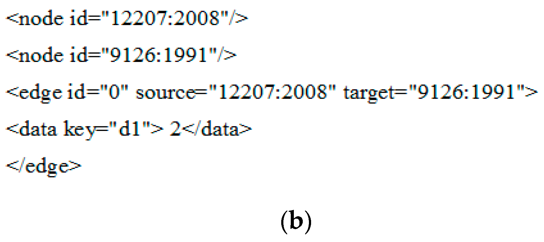
Each standard has information about its identification, referenced standard and reference type. For the purpose of this research, each standard is treated as a ‘node’. Further, a relation between a standard and its referenced standard can be established, and the relation is represented as an ‘edge’. Hence, raw data can be transferred into directed graph models. For example, in Figure 1a, “12207:2008” is a normative ISO/IEC standard. It has a referenced standard—“9126:1991”, which is an informative reference standard. Then in a graph model, the description involving those two standards and one connection is shown Figure 1b. More details are given in the ‘Method’ section.

1.3. Graph Centrality Metrics

In the scientific impact analysis, a variety of new impact measures have been proposed on the basis of network analysis and usage log data, to better capture the impact of scientific publications in the digital era. Bollen et al. [26] conducted research that investigates connections between the impact measures and those measures’ accuracy and completion. The authors applied four graph centrality metrics to analyse publication citation and usage networks. Degree centrality is used to present a number of connections that point to or emerge from a journal in the network; Closeness centrality shows the average length of the geodesic that connects a specific journal to all other journals in the network; Betweenness centrality represents the number of geodesics between all pairs of journals in the network that pass through the specific journal; and PageRank forms a probability distribution of links and is applied to citation networks. Their experimental results indicate that the notion of scientific impact is a multi-dimensional construct that cannot be adequately measured by any single indicator, although some measures are more suitable than others [26]. Similarly, graph centrality metrics have also long been used in social network analysis (SNA) to provide different perspectives on the social relationships within the network, hence offering a rich description of social structure [17]. Social networks are examples of graph data. A social network includes a set of actors and relationships among the actors. SNA has experienced tremendous advances in recent years, and much research has been reported in the literature [10,27,28,29,30,31].
In order to get a better grip on all the scientific standards (121 ISO/IEC standards in this study) collected, we conducted a study to determine which standards are at the centre of all standards, and what all the normative relations are to help users know what and where to pay attention to while revising them. Therefore, graph centrality metrics are to discover relationships among the ISO/IEC scientific standards. Note that centrality metrics can be influenced by taking into account the direction of edges and the weightings that are applied to them [32]. More specifically, six metrics are adopted based on graph models produced in our experiments, namely, Eigenvector centrality, PageRank, Weighted In-Degree, Weighted Out-Degree, Closeness and Betweenness metrics.
  • Eigenvector centrality. It is a natural extension of degree centrality. Not all nodes are equivalent. Some are more relevant than others, and reasonably, endorsements from important nodes are counted more. In other words, a node is important if it is linked to other important nodes [9,33,34,35].
  • PageRank. A node is important if it is linked from other important nodes, or if it is highly linked [36,37].
  • Weighted In-Degree centrality and Weighted Out-Degree centrality. Similar to degree centrality but edge weight is taken into account [38,39,40]. Here, In-Degree metric computes the number of incoming nodes of a vertex, and Out-Degree calculates the number of outgoing neighbours of a node.
  • Closeness centrality. For one node it can be calculated as the average distance of all distances from this node to all other nodes in the network [41]. The highest closeness node can reach every other node in a network on a short path [42].
  • Betweenness centrality. A node has high betweenness centrality if it serves as an intermediate between many other nodes, that is, it lies between them with respect to their shortest path. In other words, if we calculate the total set of shortest paths, then a node with high betweenness centrality is present with a large proportion of this set. Again, the higher this metric is, the more important the node is, since it controls the flow of information between many other nodes [41]. The highest betweenness node is on the closest link between other nodes [42].
In addition to the above centrality metrics, Modularity is also applied to measure the strength of division of a standard dataset into modules. Many graphs of interest in the science field are found to divide naturally into communities or modules. The problem of detecting and characterising this community structure is one of the outstanding issues in the study of networked systems. Modularity is a powerful tool for studying the design of networks and a highly effective approach that analyses the possible divisions of networks [43,44,45,46]. Note that in our experiment, only basic analysis of Modularity is done since the emphasis of this study is to find out the ranking of standards.

1.4. Motivations and Contributions

Many visualisation tools have all been adopted to visually exploit data insights in many application domains [47,48]. However, to the best of our knowledge, few attempts have been made to conduct visual analytics of scientific standard datasets [1,3], although some similar studies in other fields do analyse particular relevant standards. For the standard analytics in the healthcare area, seven Electronic Healthcare Record (EHR) standards were compared by Eichelberg et al. [49]. In that survey, the Web Access to Digital Imaging and Communications in Medicine Persistent Objects (WADO) standard requires a structured reporting document in HTML format, but visualisation is not mentioned. In the general case, it is not possible to support advanced services beyond document visualisation such as document processing, mediation, or automated translation services in this area [49].
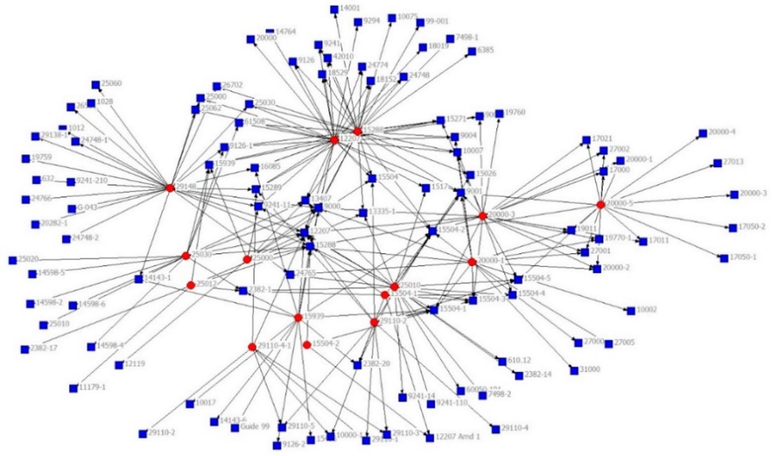
Currently, data analytics of scientific standard datasets are still conducted in the traditional spreadsheet way. The study we report in this paper was originally encouraged by the actual demand from the scientific standards management section at UTS (University of Technology Sydney); a general problem they met in this area is that this particular standards committee has a large number of standards and is losing track of how they all relate to each other. On the one hand, research has shown that visualisation can be helpful for data sense-making [11,12]. On the other hand, to get a better grip on all the standards, the centre standards and normative relations need to be determined [1,3]. Figure 2 shows a visualised result of the standard dataset that was finalised by UCINET. It shows overall relationship patterns between individual standards, which is better than traditional spreadsheets but does not bring out the importance of a standard and it also has duplicated references all over the place. Hence, this study has been put on the agenda. Our proposed approach models the standard dataset into directed graphs, adopts centrality measurement concepts for importance measurement of standards, and combines two force-directed algorithms on weighted graphs to represent an overview on the entire network of selected standards, as well as detailed views of standards.
The main contribution of our work is that we provide a supplementary method for analysis of scientific standards. More specifically this method could assist particular standards committees to get insight of complex relationships among multiple Scientific Standards; to keep track of how standards are related to each other; to determine core standards that are at the centre of the network for revising purposes and for undertsanding the impact of change. Our method combines graph centrality measurements and interactive visualisation methods and applies them to practical standard data. We performed experiments on a standard dataset to demonstrate that our method is feasible and beneficial.

2. Method

2.1. Data Processing

All raw data were collected at UTS. One hundred and twenty-one scientific standards which involve 248 relations among scientific standards were finalised. Data format examples are shown in Table 1:
From Table 1, data attributes include:
  • Standard Name: The standard’s name. E.g. 12207:2008: It is a common framework for describing the life cycle of systems created by humans, which defines a set of processes and associated terminology.
  • Standard Publisher: Standard’s publisher. E.g. 12207:2008’s publisher is ISO/IEC.
  • Standard Type: Standards can refer to other standards normatively or informatively. Normative standards contain clauses that can become contractually required; Informative standards are there to give advice.
  • Related Reference Standard: Connected standards as references. For example, standard 9126:1991 is a reference to 12207:2008.
  • Reference Type: Same as the standard type mentioned.
  • Reference Publisher: Same as the standard publisher mentioned.
  • Reference Detail: To show more information about the reference.
In this study, raw data attributes such as the standard name and related reference name are kept as vertices. Edges have directions and are represented depending on their ‘reference’ relations. Edge weights are calculated based on the standard/reference types defined in Table 2. Edges between normative standards are the most important connections as normative standards contain a number of compulsory requirements for other standards. Therefore, the weight of an edge between two normative standards is defined as 3. For example, the weight of the edge that connects standard 12207:2008 and 9126:1991 is 2, since one standard is normative and the other one is informative.
Final graph models are generated for further experiments following the GraphML (Graph Mark-up Language) format, which is an XML-based format for the description of graph structures, designed to improve tool interoperability and reduce communication overhead [13]. An XML graph file sample is given in Appendix A that also represents a graph shown in Figure 3. Eventually, relevant graph models are generated, and G1 = (V1, E1) (|V1| = 121, |E1| = 248) represents the entire network of 121 scientific standards collected.

2.2. Data Visualisation

Force-directed layout algorithms use a physical analogy to draw graphs [11,12]. A graph is viewed as a system of bodies with forces acting between the bodies. The algorithm seeks a configuration of the bodies with locally minimal energy, that is, a position for each body, such that the sum of forces on each body is zero. Graphs drawn with these force-directed algorithms tend to be aesthetically pleasing, exhibit symmetries, and most likely to produce crossing-free layouts for planar graphs [11,12,50,51,52,53,54]. To discover the centrality metrics (relationship and importance) among scientific standards, two force-directed algorithms are applied to weighted node-link graphs to represent standard network structures. Those two algorithms have strong theoretical foundations and are easy to implement, and produce good-quality results with interactive aspects. Although they tend to have a relatively long running time on large datasets, they are suitable for our experiments to handle a few hundred elements [12,55,56,57,58].

2.2.1. FR (Fruchterman and Reingold)

The Fruchterman and Reingold algorithm is a traditional force-directed layout algorithm, modified from the spring embedder model of Eades [12]. FR excels at producing aesthetically pleasing, two-dimensional graphs by doing simplified simulations of physical systems. It is simple, elegant, conceptually intuitive, and efficient, and produces uniform edge length. It comes with a high running time due to its big O notations though [55,56].

2.2.2. FA2 (ForceAtlas2)

The FA (ForceAtlas) layout algorithm [57,58] is a spatial layout method under the category of force-directed algorithms. It aims at giving a readable shape to large real-world networks, such as web networks etc. FA2 is based on FA but offers more options and innovative optimisations that make it a very fast layout algorithm. Its implementation of adaptive local and global speeds brings good performances for a network of fewer than 100,000 nodes. It is empirically observed that FA2 is at its best with strongly clustered networks [57].

2.3. Centrality Measure Model

In this study, a standard dataset is a labelled directed weighted graph G = (V, E, w), where V is the set of nodes, E is the set of edges and w is the weight function (see Section 2.1). Six centrality metrics are adopted in experiments to examine the standard’s network.
The Eigenvector centrality concept is adopted as a ranking measure to analyse the importance of standards. It attributes a value that represents the connection intensity among nodes; a higher value indicates a more important node, and a node with high eigenvector centrality is not necessarily highly linked (the node might have few but important links) [9,33,34,35]. For example, Google’s PageRank algorithm is a variant of eigenvector centrality. In this study, Eigenvector centrality measures the extent to which a standard interacts with other standards in the network. The PageRank centrality is also applied in graphs; it results from a random walk of a network. PageRank assigns probability distributions to each node denoting the importance of the node [36,37] via measuring the probability of being at that node during the random walk. At each node in a graph, the next node is chosen with probability from the set of successors of the current node (neighbours for the undirected case). If a node has no successors, the next node is chosen from all nodes, and nodes with higher importance are more likely to be chosen. Both the Weighted In-Degree centrality and the Weighted In-Degree centrality take into consideration the weights and direction of ties; both have been the preferred measures for analysing weighted and directed networks [38,39,40]. Betweenness centrality is a measure of control (nodes with high Betweenness can control other vertices more), and Closeness is a measure of access (nodes with high Closeness can access other nodes more, thus having higher influence) [42,59].

2.4. Graph Layout Generation

Graph models are imported into the Gephi tool [58] to produce final layouts. Gephi comes with interactive features such as zoom in/out, filtering, highlight etc. The entire network is laid out by the FA2 algorithm. Besides, for the purpose of showing ‘clear’ detailed relationships of selected standards, smaller graph models are represented through the FR method as well. Several visual attributes are applied to show the scientific standard’s importance (centrality):
  • Node’s colour depth: Dark green indicates larger centrality values of Weighted Degree, PageRank and Eigenvector etc., while light green represents smaller values on the opposite;
  • Node’s size: Larger size expresses larger centrality values, while smaller size indicates smaller centrality values;
  • Edge thickness: To show the edge weights: thick edges represent stronger connections while thin edges indicate weaker relations.

2.5. Hypotheses

To grasp deeper insights into the scientific standard collected, we examine the data structure and determine which scientific standards are at the centre of the whole graph. To reduce possible chance of losing track of how they relate to each other, we apply the centrality concept onto finalized graph layouts and suppose that: Force-directed algorithms could be applied to provide visualised scientific standard network representation; Centrality values could be applied to measure the importance of scientific standards, and the measurements involve not only the connectivity among standards, but also how important the related standards are. In other words, node importance is dependent on its edge degree, and which nodes it connects as well. We hypothesise that our method may assist users to track the relations among multiple scientific standards, and the users will be enabled to focus on standards of priority while revising/tracking them.

2.6. Procedure

In this study, firstly, raw data is collected in spreadsheets from UTS and then cleaned to remove typo errors and correct values. Secondly, based on the scientific standards’ reference relations and standard types, raw data is transformed into directed graph models in XML data formats. Thirdly, relevant graph models are imported into the Gephi tool, and FR and FA2 algorithms are applied to generate particular graph layouts, along with metrics attributes such as degree and eigenvector centrality etc. for further analytics. Finally, based on generated visualisations, scientific standard relations are analysed, and experimental results are discussed.

3. Results

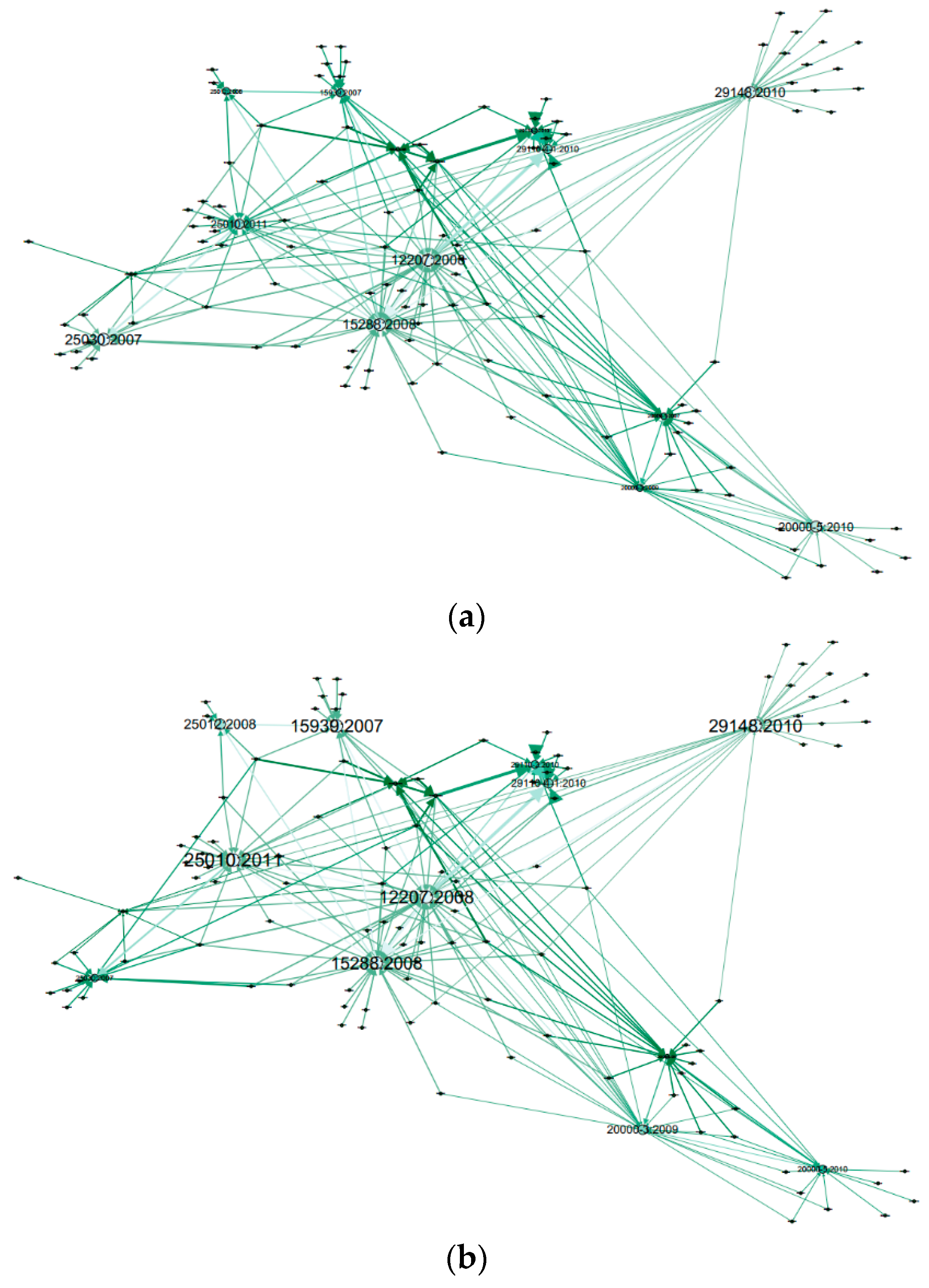
Six visualisations that are generated for the six centrality metrics are shown in Figure 3. As can be seen from Figure 3, minor differences are among all these layouts except the Weighted Out-Degree and Closeness measurements. There is nearly 80% match in the PageRank, Eigenvector, Weighted In-Degree and Betweenness centrality metrics, while the remaining two metrics represent different results.
First, it is reasonable that four metrics—PageRank, Eigenvector, Weighted In-Degree and Betweenness centrality, perform well since nodes with high in-degree are in the centre that can affect others easily [60]. The Weighted In-Degree is a measure of the system-wide influence that a particular node has; PageRank is to define a link analysis method to evaluate a node’s influence [61]; Eigenvector of a directed graph is practical for nodes with high in-degree [62]; and Betweenness centrality is a measure of control [59].
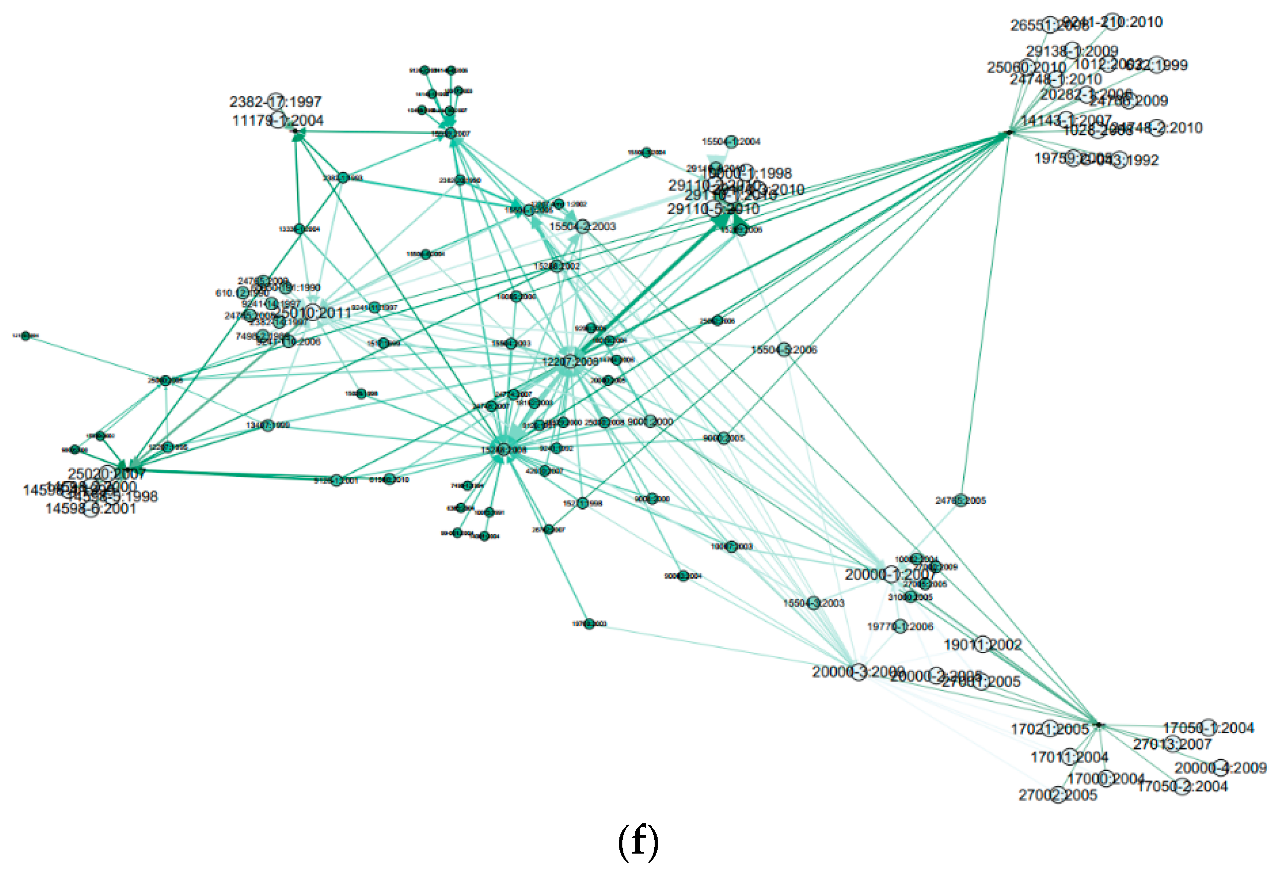
Second, it is not surprising that Weighted Out-Degree centrality and Closeness centrality are in negative correlation with standards. Here, in this study, the emphasis is to find out the standards that affect others more in the network. Nodes that have a larger Weighted Out-Degree value have more influence than other nodes [60]. Weighted Out-Degree is a measure of the system-wide influence that a node has, while Closeness indicates the access capability of a node that can be easily affected by other core nodes [59]. For example, in all visualisations in Figure 3, standards 12207:2008 and 15288:2008 are the core (most important) standards (normative standards) except the Closeness metric, yet they all have large Out-Degree as well. On the other hand, 15939:2007 plays an important role. Although it comes with less Out-Degree, it is more stable in the network. Moreover, 25 groups of similar comparisons have been processed between graph layouts and raw data collected, and they all show the importance of normative standards.
In Table 3, the top 10 standards for the six centrality metrics are given. For each standard, the standard name, centrality value and the catalogue it belongs to are included in the table. For the centrality measure, a higher value indicates a higher ranking. For example, 12207:2008’s value for the Weighted In-Degree metric is 66.0, which makes it the most ‘powerful’ node to control others. All nodes with high centrality values in PageRank, Eigenvector, Weighted In-Degree and Betweenness centrality are normative standards.
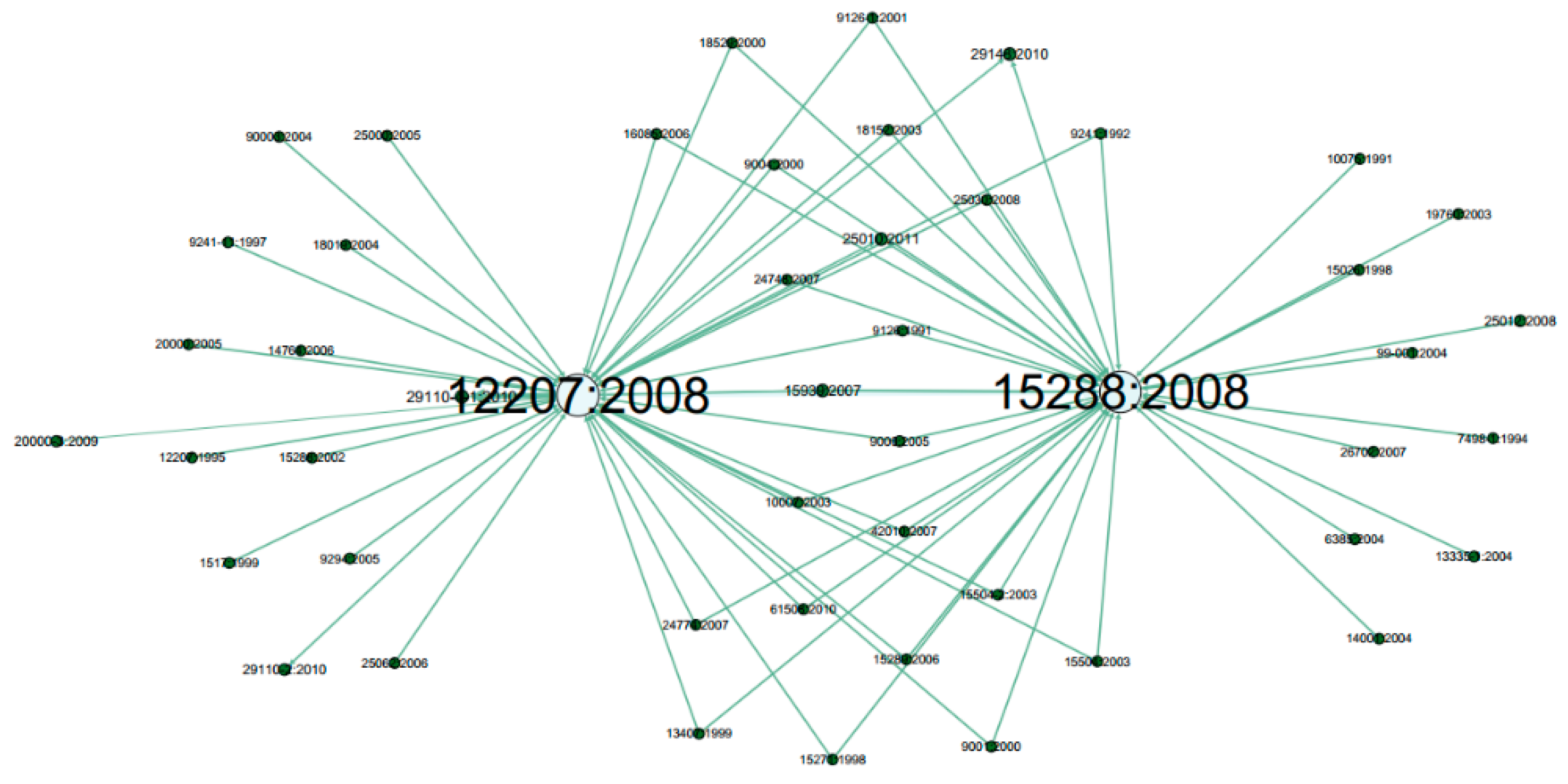
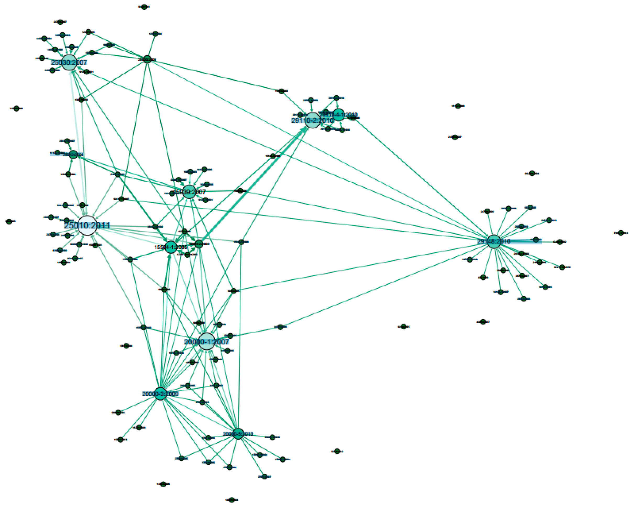
Figure 4 shows the networks of two specific standards. From Figure 4, it can be seen that the standard which has the strongest connection to 12207:2008 is 15288:2008, followed by 29110-4-1:2010. Also 12207:2008 has the highest correlation with 15288:2008, while 15939:2007 has the second highest correlation with it. Figure 5 shows the network after these two most important nodes are removed. In this entire network, 1.65% node deduction meant that 13.2% (16) other nodes lost connections, and that 30.6% (76) edges disappeared, although those ‘lonely’ nodes are distributed peripherally and are all informative standards.
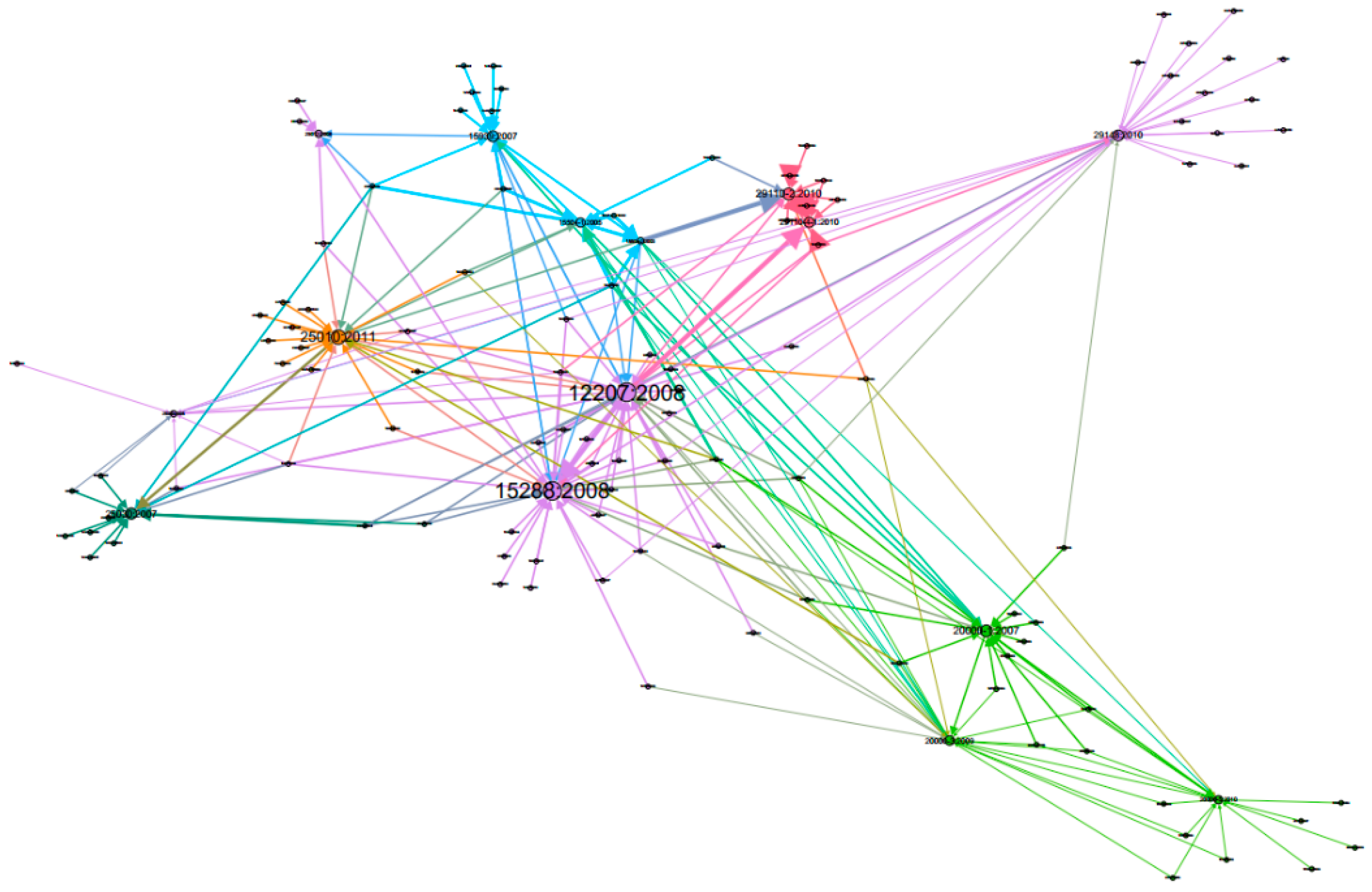
We also applied the Modularity measure in the standards dataset and six groups were identified. Broadly speaking, those standards in our study are all in the Information Technology area. Regarding the clustering of standards, nodes tend to be in the same group if they are in similar catalogues as shown in Table 4. Figure 6 shows a visualisation of the six groupings for the Weighted In-Degree measurement.

4. Discussion

Scientific standard datasets are normally complex and come with different formats and contents. More often there are multiple relations among standard items. How to track their connections has become a challenge in managing and making sense of scientific standard datasets. Although data visualisation methods have been widely applied in many sectors for decision-making purposes, they have hardly been adopted in analysing scientific standard data. To fulfil the standards management purpose, we employed an approach that allows us to conduct analytical experiments in a more practical/realistic environment.
The differences between this approach and other methods such as Excel spreadsheets that are currently used in the scientific standard analytics are as follows: This approach uses pure mathematics calculations; it addresses scientific standard relation analytics; it reduces the analytics complexity of the traditional spreadsheet methodology; this approach applies five centrality measures onto practical scientific standards analytics; it adopts two force-directed algorithms; and this approach provides a comprehensive picture of relation representation, which also has the potential to be made interactive for an overview and detailed/filtered views.
As demonstrated in our analysis in the previous section, the early outcomes of our experiments showed that modelling scientific standard datasets into graphs offers capability of recognising important standards, and that with our approach, it was possible to generate interactive and comprehensive detailed/filtered graph layouts to provide “clear“ views for users to navigate and find out item relationships they might be interested in (based on node colour, size and edge thickness etc.). Importance of scientific standards could be grasped through centrality measures (degree, eigenvector value etc.). It could also help to identify missed core (high centrality value) standards that could damage the infrastructure of a scientific standard network (see Figure 5). Further, our experimental results revealed that the standard’s importance was dependant on multiple factors. For example, nodes with more connections did not necessarily act importantly; node degree was only one of multiple metrics for importance measurement of standards.
The hypotheses were confirmed from those findings in this study. Force-directed algorithms could be adopted well to provide visual representations of the interconnected standards. In regards to the correctness of the relationship description, to be more specific, factors, such as degree and eigenvector centrality values etc. have been taken into account as well, and a standard’s importance was found to be dependent on multiple factors.
Compared to the traditional spreadsheet methodology in the scientific standard analytics, the advantages of this proposed approach include: visualisations make connection patterns of standards visual and easier to spot; the importance ranking values help identify main standard items for quick decision making; combination of centrality metrics and data visualisation methods has not been applied in analysis of scientific standard datasets to our best literature knowledge.

5. Conclusions

In this paper, an exploratory study that discovers scientific standard data is presented. We demonstrated how a scientific standard dataset can be modelled into graphs and visualised into graph drawings using force-directed algorithms with graph centrality metrics. The proposed approach is based on a practical use purpose from UTS, which is to visualise complex connections among scientific standards. Here, centrality measurement concepts and graph drawing methods are applied to practical standard data, clear relations are presented to assist the particular standards committee to track how those scientific standards relate to each other, and it is processed from a quantitative perspective in a more practical experimental setting, hence, to improve the configuration efficiency in the scientific standard management field.
More specifically, we collected sample raw data from practical scientific standards at UTS and examined the data by producing visualisations of them. Based on related scientific standard datasets collected, raw data was processed and imported for data visualisation experiments. The experimental outcomes showed that graph visualisations provide clear relations among standards compared to the spreadsheet methodology. We also showed in our visualisations the centrality measures from a quantitative perspective in a more practical experimental setting. As a result of our approach, it was shown that there are priority standards that might affect each other and could be difficult to find otherwise.
It is important to note that the benefits of applying graph centrality metrics in visual analytics of scientific standard datasets need further investigations. This is because our study has limitations. For example, raw data have not been examined via other methodologies except spreadsheet yet; data sample size is small; the accuracy of outcomes is not persuasive enough. Further, to verify the benefits of visualisations with metric measures, eye tracking studies, more well-defined interactive methods and systems can also be useful [48,63].
In our future research, we will examine a wider range of scientific standard datasets with different features. We also plan to use different visualisation algorithms and additional importance metrics to examine the standard datasets so that we could have a more comprehensive understanding of these types of datasets.

Author Contributions

Conceptualization, J.H.; Methodology, J.H. and M.L.H.; Software, J.H.; Validation, J.H., C.Z.; Formal Analysis, J.H. and W.H.; Investigation, J.H. and W.H.; Resources, J.H. and M.L.H.; Data Curation, J.H.; Writing—Original Draft Preparation, J.H.; Writing—Review & Editing, J.H. and W.H.; Visualization, J.H.

Funding

This research received no external funding.

Conflicts of Interest

The authors declare no conflict of interest.

Appendix A

//Graph model example.
<?xml version= “1.0 “ encoding= “UTF-8 “?>.
<graphml>.
<key id= “d0 “ for= “node “.
attr.name= “color “ attr.type= “string “>.
<default> yellow </default>.
</key >.
<key id= “d1 “ for= “edge “.
attr.name= “weight “ attr.type= “double “/>.
<graph id= “G “ edgedefault= “directed “>.
<node id= “12207:2008 “/>.
<node id= “9126:1991 “/>.
<node id= “25062:2006 “/>.
<node id= “61508:2010 “/>.
<node id= “10007:2003 “/>.
...
<node id= “632:1999 “/>.
<node id= “9241-210:2010 “/>.
<node id= “G-043:1992 “/>.
<edge id= “0 “ source= “9126:1991 “ target= “12207:2008 “>.
<data key= “d1 “> 2</data>.
</edge>.
<edge id= “1 “ source= “25062:2006 “ target= “12207:2008 “>.
<data key= “d1 “> 2</data>.
</edge>.
...
<edge id= “247“ source= “29148:2010 “ target= “G-043:1992 “>.
<data key= “d1 “> 1</data>.
</edge>.
</graph>.
</graphml>.

References

  1. Yarmey, L.; Baker, K.S. Towards Standardization: A Participatory Framework for Scientific Standard-Making. Int. J. Digit. Curation 2013, 8, 157–172. [Google Scholar] [CrossRef]
  2. International Organization for Standardization (ISO): ISO/IEC 12207:2008 Information Technology—Software Life Cycle Processes; ISO: Geneva, Switzerland, 2008.
  3. Ribaud, V.; Saliou, P.; Connor, R.V.O.; Laporte, C.Y. Software Engineering Support Activities for Very Small Entities. In Proceedings of the European Conference on Software Process Improvement (EuroSPI 2010), Grenoble, France, 1–3 September 2010; pp. 165–176. [Google Scholar]
  4. Yergeau, F. UTF-8, A Transformation Format of ISO 10646 (No. RFC 3629); ISO: Geneva, Switzerland, 2003. [Google Scholar]
  5. Milgram, S. Obedience to Authority. Available online: https://www.panarchy.org/milgram/obedience.html. (accessed on 19 December 2018).
  6. Woods, S.P.; Scott, J.C.; Sires, D.A.; Grant, I.; Heaton, R.K.; Tröster, A.I.; HIV Neurobehavioral Research Center (HNRC) Group. Action (verb) fluency: Test-retest reliability, normative standards, and construct validity. J. Int. Neuropsychol. Soc. 2005, 11, 408–415. [Google Scholar] [PubMed]
  7. Finkbeiner, M.; Inaba, A.; Tan, R.; Christiansen, K.; Klüppel, H.J. The new international standards for life cycle assessment: ISO 14040 and ISO 14044. Int. J. Life Cycle Assess. 2006, 11, 80–85. [Google Scholar] [CrossRef]
  8. Kenny, D. ISO and CEN documents on quality in medical laboratories. Clin. Chim. Acta 2001, 309, 121–125. [Google Scholar] [CrossRef]
  9. Lohmann, G.; Margulies, D.S.; Horstmann, A.; Pleger, B.; Lepsien, J.; Goldhahn, D.; Schloegl, H.; Stumvoll, M.; Villringer, A.; Turner, R. Eigenvector centrality mapping for analyzing connectivity patterns in fMRI data of the human brain. PLoS ONE 2010, 5, e10232. [Google Scholar] [CrossRef] [PubMed]
  10. Batagelj, V.; Andrej, M. Pajek—Analysis and visualization of large networks. In International Symposium on Graph Drawing; Springer: Berlin/Heidelberg, Germany, 2001; pp. 477–478. [Google Scholar]
  11. Battista, G.D.; Eades, P.; Tamassia, R.; Tollis, I.G. Graph Drawing Algorithms for the Visualization of Graphs; PrenticeHall: Upper Saddle River, NJ, USA, 1999. [Google Scholar]
  12. Eades, P. A heuristic for graph drawing. Congr. Numer. 1984, 42, 149–160. [Google Scholar]
  13. Huang, W.; Huang, M.L.; Lin, C.-C. Evaluating Overall Quality of Graph Visualizations Based on Aesthetics Aggregation. Inf. Sci. 2016, 330, 444–454. [Google Scholar] [CrossRef]
  14. Huang, M.L.; Huang, W. Innovative Approaches of Data Visualization and Visual Analytics; IGI Group: Hershey, PA, USA, 2014; 464p. [Google Scholar]
  15. Huang, T.-H.; Huang, M.L.; Nguyen, Q.V.; Zhao, L.; Huang, W.; Chen, J. A Space-Filling Multidimensional Visualization (SFMDVis) for Exploratory Data Analysis. Inf. Sci. 2017, 390, 32–53. [Google Scholar] [CrossRef]
  16. Hua, J.; Huang, M.L.; Huang, W.; Wang, J.; Nguyen, Q.V. Force-directed graph visualization with pre-positioning-Improving convergence time and quality of layout. In Proceedings of the 16th International Conference on Information Visualisation, Montpellier, France, 11–13 July 2012; pp. 124–129. [Google Scholar]
  17. Brandes, U.; Wagner, D. Analysis and visualisation of social networks. In Graph Drawing Software; Springer: Berlin/Heidelberg, Germany, 2004; pp. 1–20. [Google Scholar]
  18. Handcock, M.S.; Hunter, D.R.; Butts, C.T.; Goodreau, S.M.; Morris, M. Statnet: Software Tools for the Representation, Visualisation, Analysis and Simulation of Network Data. J. Stat. Softw. 2005, 14, 1–11. [Google Scholar] [CrossRef]
  19. Ripley, R.; Boitmanis, K.; Snijders, T.A.B. RSiena: Siena—Simulation Investigation for Empirical Network Analysis. R Package Version 1.1-232. 2013. Available online: http://CRAN.R-project.org/package=RSiena (accessed on 19 December 2018).
  20. Csárdi, G.; Nepusz, T. The igraph software package for complex network research. Int. J. Comp. Syst. 2006, 1695, 1–9. [Google Scholar]
  21. Borgatti, S.P.; Everett, M.G.; Freeman, L.C. UCINET 6.0 Version 1.00; Analytic Technologies: Natick, MA, USA, 1999. [Google Scholar]
  22. Hansen, D.L.; Shneiderman, B.; Smith, M.A. Analyzing Social Media Networks with NodeXL: Insights from a Connected World; Morgan Kaufmann: Burlington, MA, USA, 2010. [Google Scholar]
  23. Kolaczyk, E.D.; Csardi, G. Statistical Analysis of Network Data with R. J. Stat. Softw. 2005, 14, 1–6. [Google Scholar]
  24. Grunspan, D.Z.; Wiggins, B.L.; Goodreau, S.M. Understanding classrooms through social network analysis: A primer for social network analysis in education research. CBE Life Sci. Educ. 2014, 13, 167–178. [Google Scholar] [CrossRef] [PubMed]
  25. Rossi, R.A.; Ahmed, N.K. The Network Repository: An Interactive Data Repository with Multi-scale Visual Analytics. In Proceedings of the Twenty-Ninth AAAI Conference on Artificial Intelligence, Austin, TX, USA, 25–30 January 2015; pp. 4292–4293. [Google Scholar]
  26. Bollen, J.; van de Sompel, H.; Hagberg, A.; Chute, R. A Principal Component Analysis of 39 Scientific Impact Measures. PLoS ONE 2009, 4, e6022. [Google Scholar] [CrossRef] [PubMed]
  27. Newman, J.R. Leonhard Euler and the Konigsberg Bridges. Sci. Am. 1953, 189, 66–70. [Google Scholar]
  28. Huang, W.; Hong, S.H.; Eades, P. Effects of sociogram drawing conventions and edge crossings in social network visualization. J. Graph Algorith. Appl. 2007, 11, 397–429. [Google Scholar] [CrossRef]
  29. Watts, D.J.; Strogatz, S.H. Collective dynamics of ‘small-world’ networks. Nature 1998, 6684, 440–442. [Google Scholar] [CrossRef] [PubMed]
  30. Baraba, A.; Albert, R. Emergence of scaling in random networks. Science 1999, 286, 509–513. [Google Scholar]
  31. Freeman, L. The Development of Social Network Analysis: A Study in the Sociology of Science; Empirical Press: Vancouver, BC, USA, 2004. [Google Scholar]
  32. Friedkin, N.E. Theoretical foundations for centrality measures. Am. J. Sociol. 1991, 96, 1478–1504. [Google Scholar] [CrossRef]
  33. Eigenvector Centrality. Available online: https://www.sci.unich.it/~francesc/teaching/network/eigenvector.html (accessed on 19 December 2018).
  34. Du, D. Social Network Analysis: Centrality Measures. Available online: http://www2.unb.ca/~ddu/6634/Lecture_notes/Lecture_4_centrality_measure.pdf. (accessed on 19 December 2018).
  35. Bonacich, P. Some unique properties of eigenvector centrality. Soc. Netw. 2007, 29, 555–564. [Google Scholar] [CrossRef]
  36. Page, L.; Brin, S.; Motwani, R.; Winograd, T. The Pagerank Citation Ranking: Bringing Order to the Web; Stanford InfoLab: Stanford, CA, USA, 1998. [Google Scholar]
  37. Langville, A.N.; Meyer, C.D. Google’s PageRank and Beyond: The Science of Search Engine Rankings; Princeton University Press: Princeton, NJ, USA, 2011. [Google Scholar]
  38. Barrat, A.; Barthelemy, M.; Pastor-Satorras, R.; Vespignani, A. The architecture of complex weighted networks. Natl. Acad. Sci. USA 2004, 101, 3747–3752. [Google Scholar] [CrossRef] [Green Version]
  39. Opsahl, T.; Agneessens, F.; Skvoretz, J. Node Centrality in Weighted Networks: Generalizing degree and shortest paths. Soc. Netw. 2010, 32, 245–251. [Google Scholar] [CrossRef]
  40. Tang, X.; Wang, J.; Zhong, J.; Pan, Y. Predicting essential proteins based on weighted degree centrality. IEEE/ACM Trans. Comput. Biol. Bioinform. 2014, 11, 407–418. [Google Scholar] [CrossRef] [PubMed]
  41. Newman, M. The Mathematics of Networks; University of Michigan: Ann Arbor, MI, USA, 2002. [Google Scholar]
  42. Krebs, V. Power in Networks. 2004. Available online: http://www.orgnet.com (accessed on 12 December 2018).
  43. Yoon, J.; Blumer, A.; Lee, K. An algorithm for modularity analysis of directed and weighted biological networks based on edge-betweenness centrality. Bioinformatics 2006, 22, 3106–3108. [Google Scholar] [CrossRef] [PubMed] [Green Version]
  44. da Silva, M.R.; Ma, H.; Zeng, A.P. Centrality, network capacity, and modularity as parameters to analyze the core-periphery structure in metabolic networks. Proc. IEEE 2008, 96, 1411–1420. [Google Scholar] [CrossRef]
  45. de Domenico, M.; Solé-Ribalta, A.; Cozzo, E.; Kivelä, M.; Moreno, Y.; Porter, M.A.; Gómez, S.; Arenas, A. Mathematical formulation of multilayer networks. Phys. Rev. X 2013, 3, 041022. [Google Scholar] [CrossRef]
  46. Newman, M.E. Modularity and community structure in networks. Proc. Natl. Acad. Sci. USA 2006, 103, 8577–8582. [Google Scholar] [CrossRef] [PubMed] [Green Version]
  47. Parsons, P.; Sedig, K.; Didandeh, A.; Khosravi, A. Interactivity in Visual Analytics: Use of Conceptual Frameworks to Support Human-Centered Design of a Decision-Support Tool. In Proceedings of the 48th Hawaii International Conference on System Sciences (HICSS), Kauai, HI, USA, 5–8 January 2015; pp. 1138–1147. [Google Scholar]
  48. Sedig, K.; Parsons, P. Design of Visualizations for Human-Information Interaction: A Pattern-Based Framework; Morgan & Claypool Publishers: San Rafael, CA, USA, 2016. [Google Scholar]
  49. Eichelberg, M.; Aden, T.; Riesmeier, J. A Survey and Analysis of Electronic Healthcare Record Standards. ACM Comput. Surv. 2005, 37, 277–315. [Google Scholar] [CrossRef]
  50. Huang, W.; Huang, M.; Lin, C. Aesthetic of Angular Resolution for Node-Link Diagrams: Validation and Algorithm. In Proceedings of the IEEE Symposium on Visual Languages and Human-Centric Computing (VL/HCC’11), Pittsburgh, PA, USA, 18–22 September 2011; pp. 18–22. [Google Scholar]
  51. Huang, W.; Eades, P.; Hong, S.H.; Lin, C.C. Improving Force-Directed Graph Drawings by Making Compromises Between Aesthetics. In Proceedings of the IEEE Symposium on Visual Languages and Human-Centric Computing (VL/HCC 2010), Leganes, Spain, 21–25 September 2010; pp. 176–183. [Google Scholar]
  52. Huang, W.; Huang, M. Exploring the Relative Importance of Number of Edge Crossings and Size of Crossing Angles: A Quantitative Perspective. Int. J. Adv. Intell. 2011, 3, 25–42. [Google Scholar]
  53. Omote, H.; Sugiyama, K. Force-Directed Drawing Method for Intersecting Clustered Graphs. In Proceedings of the 6th International Asia-Pacific Symposium on Visualization, Sydney, Australia, 5–7 February 2007; pp. 85–92. [Google Scholar]
  54. Lin, C.C.; Yen, H.C. A New Force-Directed Graph Drawing Method Based on Edge-Edge Repulsion. In Proceedings of the Ninth International Conference on Information Visualisation, London, UK, 6–8 July 2005; pp. 329–334. [Google Scholar]
  55. Kobourov, S.G. Force-directed drawing algorithms. In Handbook of Graph Drawing and Visualization (Discrete Mathematics and Its Applications); CRC Press: Boca Raton, FL, USA, 2013; pp. 383–408. [Google Scholar] [CrossRef]
  56. Gansner, E.R.; North, S.C. Improved force-directed layouts. In Proceedings of the International Symposium on Graph Drawing and Network Visualization, Montreal, QC, Canada, 13–15 August 1998; pp. 364–373. [Google Scholar]
  57. Jacomy, M.; Heymann, S.; Venturini, T.; Bastian, M. Force Atlas 2, A Graph Layout Algorithm for Handy Network Visualisation. Available online: https://journals.plos.org/plosone/article?id=10.1371/journal.pone.0098679. (accessed on 19 December 2018).
  58. Bastian, M.; Heymann, S.; Jacomy, M. Gephi: An Open Source Software for Exploring and Manipulating Networks. In Proceedings of the Third International ICWSM Conference, San Jose, CA, USA, 17–20 May 2009. [Google Scholar]
  59. Schiffer, E.; Hauck, J. Net-Map: Collecting Social Network Data and Facilitating Network Learning through Participatory Influence Network Mapping. Field Methods 2010, 22, 231–249. [Google Scholar] [CrossRef]
  60. Gao, Y.C.; Zeng, Y.; Cai, S.M. Influence network in the Chinese stock market. J. Stat. Mech. Theory Exp. 2015, 2015, P03017. [Google Scholar] [CrossRef]
  61. Li, J.; Peng, W.; Li, T.; Sun, T.; Li, Q.; Xu, J. Social network user influence sense-making and dynamics prediction. Expert Syst. Appl. 2014, 41, 5115–5124. [Google Scholar] [CrossRef]
  62. Newman, M. Networks: An Introduction; Oxford University Press: Oxford, UK, 2010. [Google Scholar]
  63. Huang, W. An Eye Tracking Study into the Effects of Graph Layout. Available online: https://arxiv.org/pdf/0810.4431.pdf. (accessed on 19 December 2018).
Figure 1. (a) Scientific standard examples in a spreadsheet; (b) an XML representation of a two-node graph.
Symmetry 11 00030 g001aSymmetry 11 00030 g001b
Figure 2. A visualisation example of the scientific standards from a previous study at UTS (finalised by UCINET).
Symmetry 11 00030 g002
Figure 3. Visualisations of a standard graph for all measurements (FA2, |E| = 121, |V| = 248). Node size, colour depth and label size indicate standard rankings. For example, nodes with the larger size, darker green colour and larger label size are more important standards with higher rankings. (a) PageRank measurement (25030:2007 is the highest-ranking standard); (b) Eigenvector centrality measurement (25010:2011 is the highest-ranking standard); (c) Weighted In-Degree measurement (12207:2008 is the highest-ranking standard); (d) Weighted Out-Degree measurement (12207:2008 is the highest-ranking standard); (e) Betweenness measurement (12207:2008 is the highest-ranking standard); (f) Closeness measurement (Top ten ranking standards have the same value).
Symmetry 11 00030 g003aSymmetry 11 00030 g003bSymmetry 11 00030 g003c
Figure 4. Standards 15288:2008 and 12207:2008’s network (FA2 applied, finalised by the Weighted In-Degree measurement, |E| = 49, |V| = 76).
Symmetry 11 00030 g004
Figure 5. Standards’ network after removing 12207:2008 and 15288:2008 (FA2 applied, finalised by the Weighted In-Degree measurement, |E| = 119, |V| = 172).
Symmetry 11 00030 g005
Figure 6. Standards’ network after applying the modularity method. (FA2 applied, finalised by the Weighted In-Degree measurement with six colours indicating six different groups of standards).
Symmetry 11 00030 g006
Table 1. Examples of standard data format finalised from excel files.
StandardRelated Reference
NamePublisherTypeNameTypePublisherDetail
12207:2008ISO/IECNormative9126:1991InformativeISO/IECBibliography
12207:2008ISO/IECNormative61508:2010InformativeIECOther citation
Table 2. Edge weight description based on standard types.
Standard RelationsEdge Weight
Normative Standard—Normative Standard3
Normative Standard—Informative Standard2
Informative Standard—Informative Standard1
Table 3. Top 10 standards with high centrality values for the six metrics.
PageRankEigenvector Centrality
StandardValueCatalogueStandardValueCatalogue
125030:20070.074Software engineering—Software product Quality Requirements and Evaluation (SQuaRE)—Quality requirements25010:20111Systems and software engineering—SQuaRE—System and software quality models
212207:20080.072Systems and software engineering—Software life cycle processes12207:20080.981Systems and software engineering—Software life cycle processes
315288:20080.071Systems and software engineering—System life cycle processes29148:20100.967Systems and software engineering—Life cycle processes—Requirements engineering
429148:20100.069Systems and software engineering—Life cycle processes—Requirements engineering15939:20070.962Systems and software engineering—Measurement process
520000-5:20100.064Information technology—Service management—Part 5: Exemplar implementation plan for ISO/IEC 20000-115288:20080.956Systems and software engineering—System life cycle processes
625010:20110.057Systems and software engineering—SQuaRE—System and software quality models25012:20080.798Software engineering—SQuaRE—Data quality model
729110-4-1:20100.048Software engineering—Lifecycle profiles for Very Small Entities (VSEs)—Part 4-1: Profile specifications: Generic profile group20000-3:20090.700Information technology—Service management—Part 3: Guidance on scope definition and applicability of ISO/IEC 20000-1
815939:20070.044Systems and software engineering—Measurement process29110-4-1:20100.656Software engineering—Lifecycle profiles for VSEs—Part 4-1: Profile specifications: Generic profile group
925012:20080.035Software engineering—SQuaRE—Data quality model20000-5:20100.524Information technology—Service management—Part 5: Exemplar implementation plan for ISO/IEC 20000-1
1020000-3:20090.034Information technology—Service management—Part 3: Guidance on scope definition and applicability of ISO/IEC 20000-129110-2:20100.504Software engineering—Lifecycle profiles for VSEs—Part 2: Framework and taxonomy
Weighted In-DegreeWeighted Out-Degree
StandardValueCatalogueStandardValueCatalogue
112207:200866.0Systems and software engineering—Software life cycle processes12207:20081Systems and software engineering—SQuaRE—System and software quality models
215288:200865.0Systems and software engineering—System life cycle processes15504-2:20030.981Information technology—Process assessment—Part 2: Performing an assessment
325010:201146.0Systems and software engineering—SQuaRE—System and software quality models15288:20020.967Systems engineering—System life cycle processes
420000-1:200734.0Information technology—Service management15289:20060.962Systems and software engineering—Content of systems and software life cycle process information products (Documentation)
529110-2:201033.0Software engineering—Lifecycle profiles for VSEs—Part 2: Framework and taxonomy9001:20000.956Quality management systems—Requirements
625030:200731.0Software engineering—SQuaRE—Quality requirements2382-1:19930.798Information technology—Vocabulary—Part 1: Fundamental terms
715939:200729.0Systems and software engineering—Measurement process15288:20080.700Systems and software engineering—System life cycle processes
829148:201029.0Systems and software engineering—Life cycle processes—Requirements engineering15504-1:20050.656Information technology—Process assessment—Part 1: Concepts and vocabulary
929110-4-1:201026.0Software engineering—Lifecycle profiles for VSEs—Part 4-1: Profile specifications: Generic profile group9000:20050.524Quality management systems—Fundamentals and vocabulary
1020000-3:200923.0Information technology—Service management—Part 3: Guidance on scope definition and applicability of ISO/IEC 20000-129110-1:20100.504Software engineering—Lifecycle profiles for VSEs—Part 1: Overview
Betweenness CentralityCloseness Centrality
StandardValueCatalogueStandardValueCatalogue
112207:2008297.4Systems and software engineering—Software life cycle processes25010:20111.0Systems and software engineering—SQuaRE—System and software quality models
215288:2008153.2Systems and software engineering—System life cycle processes20000-3:20091.0Information technology—Service management—Part 3: Guidance on scope definition and applicability of ISO/IEC 20000-1
315939:200787.93Systems and software engineering—Measurement process20000-1:20071.0Information technology—Service management
425010:201160.0Systems and software engineering—SQuaRE—System and software quality models29110-2:20101.0Software engineering—Lifecycle profiles for VSEs—Part 2: Framework and taxonomy
520000-3:200950.67Information technology—Service management—Part 3: Guidance on scope definition and applicability of ISO/IEC 20000-119011:20021.0Guidelines for auditing management systems
615504-1:200534.03Information technology—Process assessment—Part 1: Concepts and vocabulary27001:20051.0Information technology—Security techniques—Information security management systems—Requirements
725000:200532.66Software Engineering—Software product Quality Requirements and Evaluation (SQuaRE)—Guide to SQuaRE20000-2:20051.0Information technology—Service management—Part 2: Code of practice
815504-2:200321.73Information technology—Process assessment—Part 2: Performing an assessment17011:20041.0Conformity assessment—General requirements for accreditation bodies accrediting conformity assessment bodies
920000-1:200715.17Information technology—Service management17021:20051.0Conformity assessment—Requirements for bodies providing audit and certification of management systems
1029110-2:20106.17Software engineering—Lifecycle profiles for VSEs—Part 2: Framework and taxonomy27002:20051.0Information technology—Security techniques—Code of practice for information security management
Table 4. Standard clustering description (modularity measurement applied, six groups finalised).
Group 012207:2008, 9126:1991, 25062:2006, 12207:1995, 13407:1999, 14764:2006, 15271:1998, 15288:2008, 15504:2003, 16085:2006, 18019:2004, 18152:2003, 18529:2000, 20000:2005, 24748:2007, 24774:2007, 25000:2005, 25030:2008, 42010:2007, 90003:2004, 9004:2000, 9241:1992, 9241-11:1997, 9294:2005, 10075:1991, 13335-1:2004, 14001:2004, 19760:2003, 26702:2007, 6385:2004, 7498-1:1994, 99-001:2004, 12119:1994, 25012:2008, 11179-1:2004, 2382-17:1997, 29148:2010, 1012:2002, 25060:2010, 26551:2008, 1028-2008, 14143-1:2007, 19759:2005, 20282-1:2006, 24748-1:2010, 24748-2:2010, 24766:2009, 29138-1:2009, 632:1999, 9241-210:2010, G-043:1992
Group 115288:2002, 15504-2:2003, 15939:2007, 15504-1:2005, 12207-1:2002, 15504-3:2004, 2382-1:1993, 2382-20:1990, 10017:2003, 14143-1:1998, 14143-6:2006, 15498:1996, 9126-2:2001, 2315-99:2007
Group 210007:2003, 9000:2005, 9001:2000, 20000-1:2007, 10002:2004, 19011:2002, 24765:2005, 27001:2005, 27005:2005, 31000:2005, 15504-3:2003, 19770-1:2006, 20000-2:2005, 27000:2009, 20000-3:2009, 17011:2004, 17021:2005, 27002:2005, 17000:2004, 20000-5:2010, 27013:2007, 17050-1:2004, 17050-2:2004, 20000-4:2009
Group 31517:1999, 15026:1998, 15504-4:2004, 15504-5:2006, 25010:2011, 24765:2008, 2382-14:1997, 24765:2009, 60050-191:1990, 610.12:1990, 7498-2:1989, 9241-110:2006, 9241-14:1997
Group 461508:2010, 9126-1:2001, 15939:2002, 9000:2000, 25030:2007, 14598-2:2000, 14598-4:1999, 14598-5:1998, 14598-6:2001, 25020:2007
Group 515289:2006, 29110-2:2010, 10000-1:1998, 15504-1:2004, 29110-1:2010, 29110-3:2010, 29110-4:2010, 29110-5:2010, 29110-4-1:2010