Spacetime Symmetries and Classical Mechanics

Abstract

Physics students are rarely exposed to the style of thinking that goes into theoretical developments in physics until late in their education. In this work, we present an alternative to the traditional statement of Newton’s second law that makes theory questions accessible to students early in their undergraduate studies. Rather than a contrived example, the model considered here arises from a popular framework for testing Lorentz symmetry used extensively in contemporary experiments. Hence, this work also provides an accessible introduction to some key ideas in ongoing tests of fundamental symmetries in physics.

1. Introduction

Is Newton’s second law obvious? Some introductory physics students respond in the affirmative. The idea that a force applied to a body results in an acceleration in proportion to the (constant) mass of the body seems to them a clear description of the way nature must work. Here, we argue that the answer ought to be “no”. We do so by developing a model that contains violations of rotation invariance. Though we develop the model from basic Newtonian-physics considerations, we arrive at the Newtonian limit of a quantum-field-theory based test framework known as the Standard-Model Extension (SME) [1,2,3]. The SME has been used extensively in searching for violations of Lorentz symmetry (invariance under boosts as well as rotations) in nature [4] with the goal of finding evidence of new physics, such as string theory [5,6].

The construction of physical theories can be thought of as a logical structure, which begins with primitive notations or undefined terms, defines additional concepts from them, and then makes assumptions about how the concepts (defined and undefined) behave. These assumptions are then tested against experimental and observational data to see if the theory so constructed is a description of a physical effect. It is sometimes hard for students and physicists alike to see theories like Newton’s laws, which have been around a long time, as fitting this form. This difficulty can make studying the subject feel separate from doing modern science. Newton’s laws have also been identified as a particularly challenging example of physical theory [7]. Presenting students with viable alternatives to standard Newtonian theory can help bring the thought processes involved in doing theoretical physics into the undergraduate classroom.

Old ideas in physics can also be difficult to test because physicists have trouble imagining how to do physics without them. Those new to the field of Lorentz-symmetry testing must work to imagine nature without perfect Lorentz symmetry. Rotation invariance is more visual than boost invariance, and it can be readily explored with Newtonian physics. Hence, one can build intuition for symmetry violation with the Newtonian limit of contemporary models of Lorentz-symmetry violation. Testing Lorentz symmetry is an active area of contemporary physics research, and this work provides an accessible introduction to some of its foundational ideas for undergraduates and those new to the field.

In this work, we develop an alternative version of Newton’s second law by lifting the assumption of isotropy. In Section 2, we develop the rotation-invariance-violating model from Newtonian considerations, and we address the use of such models in stimulating classroom discussion about the theoretical-physics aspects of Newton’s laws. Section 3 introduces the idea of the SME and discusses how our alternative version of Newton’s second law fits into it. In Section 4, we explore an example that provides some intuition for how to do physics with the alternative law as well as for how tests of spacetime symmetries are developed. Finally, Section 5 demonstrates the connection between spacetime symmetries and conserved quantities using our alternative Newton’s second law as an explicit example.

2. Alternative Newton’s Second Laws

A common statement of Newton’s second law found in introductory physics courses proceeds as follows: the net force $\overrightarrow{F}$ applied to a body is proportional to the acceleration $\overrightarrow{a}$ of that body. The proportionality factor, typically taken as constant at this stage, is known as the mass m. The easiest way to imagine an alternative to Newton’s second law is to provide a more general form that reduces to the original in some limit. In this section, we consider such examples.

We frame these alternatives in the language above with unaltered force laws such that the simplest limits of our examples may be accessible to students at this level. There are a variety of interpretations of Newton’s second law [8]. Hence, some readers might prefer to use $\overrightarrow{F}=\frac{d\overrightarrow{p}}{dt}$ as the definition of Newton’s second law, while recasting the examples to follow as proposed alternative forms for the conserved momentum. Others might wish to interpret the effects we consider as changes to the force laws. We address some of these possibilities in the sections to follow.

Consider first a rotation-invariance-violating (RIV) model with a constant mass. Suppose one applies a given force to a body at rest. One could imagine, for example, that our standard force is defined by stretching a given spring a particular distance. Suppose that the body experiences an instantaneous acceleration a in response to our applied force. Now, suppose that the system is rotated 90 degrees, such that our standard force is applied in a new direction, and in the new configuration a different acceleration, $a^{\prime }$, results. If such an observation were made, one could imagine modeling it with two Newton’s second laws, one for the east–west direction

$$F=ma,$$

(1)

and one for the north–south direction

$$F=m^{\prime }{a}^{\prime },$$

(2)

with bodies now having two properties, east–west mass m and north–south mass $m^{\prime }$. This is a clear violation of rotation invariance. One is then faced with the question of what happens when the system is rotated, not by 90 degrees, but by some other angle. The natural extension is to write Newton’s second law in the form

$$F_j=m_{jk}{a}_k,$$

(3)

where Einstein summation convention has been used. In this model, we take $m_{jk}$ as symmetric. While one can consider antisymmetric contributions to $m_{jk}$ here at the level of Newton’s second law, such contributions prevent the definition of a kinetic term and hence such models appear to lie outside of action-based theory. We also assume this matrix is invertible. Under these conditions, one finds that forces exerted along three special directions produce accelerations aligned with the force while forces exerted in other directions produce no such alignment. Note that coordinates can always be found that diagonalize the matrix. In these special coordinates, forces aligned with the coordinate axes will produce accelerations aligned with the force and the full model reduces to the original idea introduced in Equations (1) and (2).

Introducing this model to students in mechanics courses produces stimulating discussion that simulates the thinking that happens in theoretical physics. Such discussions can be provoked by asking questions such as, “is this alternative experimentally viable, or has it been ruled out?”, “is it internally consistent?”, or “how could it be distinguished experimentally from the ‘usual’ form?”. Depending on the level of the course, the presentation can be simplified by using matrix form, and/or using diagonalizing coordinates up front.

Though it has not been confirmed by experiment to date, the RIV model is not pure fiction as it has a clear connection to ongoing efforts in contemporary physics as we discuss in the next section. Such connections can be used to bring recent literature into the classroom. Using notation suggestive of the development to follow, the RIV can be rewritten in the form:

$$F_j=m({\delta }_{jk}+2c_{jk})a_k.$$

(4)

Here, an overall factor m equal to 1/3 of the trace of $m_{jk}$ has been pulled out of $m_{jk}$, and the remaining matrix has been written as the identity (Kronecker delta) plus a traceless matrix $2c_{jk}$. Though we could always choose to write $m_{jk}$ in the form above, this form is particularly convenient when thinking of $c_{jk}$ as a small anisotropic correction to the usual isotropic mass as is typically demanded by existing experimental constraints such as spectroscopy measurements. This form also makes it clear that the model will always be viable for sufficiently small $c_{jk}$.

The discussion around physical theories and Newton’s second law in mechanics courses can be further enhanced by introducing additional examples, which, rather than rotation invariance violation, introduce other modifications. Consider a proportionality factor between the force and acceleration that is a function of some quantity, say the velocity. Hence experimentally, when the same force is applied to a given body (in the lab frame), different accelerations result depending on the velocity the body has at the instant when the force is applied. Consider the following example:

$$F_i=m\left(\gamma {\delta }_{ij}+\frac{1}{c^2}{\gamma }^3{v}_i{v}_j\right)a_j,$$

(5)

where

$$\gamma =\frac{1}{\sqrt{1-\frac{v^2}{c^2}}},$$

(6)

and c is a constant with units of velocity. Note that in the limit $v<<c$, this alternative would be experimentally indistinguishable from the ordinary case. Hence, for a sufficiently large value of c, this model would remain experimentally viable even if no such velocity dependence were present in nature. Some readers may recognize Equation (5) as a special-relativistic version of Newton’s second law [9] common in undergraduate treatments [10]. Introducing this result, or perhaps more appropriately one of its simpler limiting forms such as the case where $\overrightarrow{v}$ and $\overrightarrow{a}$ are aligned,

$$F=m{\gamma }^{3}a,$$

(7)

to students not familiar with special relativity (without saying initially that it’s special relativity) produces another model to which the above discussion questions can be applied. Moreover, it demonstrates convincingly that the original notion of Newton’s second law is not obvious. For the implication involved in calling something obvious, is that it is obviously right. Since Equation (5) is more correct than the original version, it seems that the original version cannot be obvious. Note that Equation (5) fits the basic form of Equation (3), but the $m_{jk}$ are no longer constant. Note also that, although this match can be made, the directionality in the effective mass in the case of Equation (5) originates from the velocity of the particle in the lab frame, rather than a fundamental violation of rotation invariance. This distinction can be further clarified using the methods to follow in Section 4.

3. The Standard-Model Extension

Among the most fundamental goals of contemporary theoretical physics is the unification of the gravitational interaction with the other three interactions in nature into a single quantum-consistent theory. Several decades ago, the realization that some such unification efforts could generate violations of Lorentz symmetry [5,6] triggered an intense renewed interest in tests of this fundamental spacetime symmetry [4] and the development of a comprehensive test framework for organizing the search [1,2]. This framework is the SME. The idea behind the SME is to add all Lorentz-violating terms to the equations of known physics to form a structure similar to a series expansion about our current best theories. The additional terms can then be sought in experiment. Though the SME expansion is quantum field theory based, the idea is analogous to the addition of $c_{jk}$ to Newton’s second law in Equation (4). One could imagine a researcher in Newtonian times proposing Equation (4) as a test framework for deviations for Newtonian physics and seeking $c_{jk}$ in experiments. Such an effort could in principle have discovered either of the models of Section 2. This connection is more than an analogy as the RIV model arises as a subset of the Newtonian limit of the SME. In the remainder of this section, we provide some comments on the connections between the RIV model of Section 2 and the SME, and provide some SME-inspired insights on the RIV model. Some more advanced discussion of the SME is provided in the Appendix A.

In developing the RIV model, we simply imagined the motion of a particle governed by different masses when moving in different directions as modeled by the matrix $m_{jk}$ or equivalently $c_{jk}$. However, one can visualize objects such as $c_{jk}$ as providing an anisotropy [11] to empty spacetime itself, and the existence of such a condensate of tensors in empty spacetime can be triggered by spontaneous symmetry breaking [12] in analogy with the scalar Higgs field in the Standard Model. The background ovals in Figure 1 illustrate this background condensate.

Via the SME connection, it is straightforward to read off the current experimental limits [4] on how anisotropic the mass in the RIV model can be. The current limits on $c_{jk}$ would permit mass anisotropies (differences in inertia among experiments performed in different directions) at roughly the parts in ${10}^{17}$ level in Newtonian experiments in an Earth-based laboratory with conventional macroscopic matter. The least constrained contribution to this number comes from the electron contribution in matter as limited by ion trapping and atomic spectroscopy experiments [13,14]. Proton and neutron contributions are more tightly constrained by a number of tests. Magnetometer experiments [15,16], a type of clock comparison [17,18,19,20], are currently the most sensitive.

4. An Example

In this section, we consider one of the most famous examples in physics, the problem of a block on an inclined plane without friction, as a simple example that illustrates some of the interesting features that arise when Newton’s second law is generalized to allow rotation-invariance violation [21]. In addition to providing some intuition for the RIV model, the example is of interest for several reasons. It provides what is perhaps the simplest example of some of the conceptual challenges that arise throughout the field of spacetime symmetry testing, some of which are quite foundational to theoretical-physics work more broadly. It is also an interesting example for mechanics students because it forces one to apply a theory without relying on potentially erroneous intuitions.

4.1. Basics

We begin with the simplest case as a starting point for working with nontrivial $m_{jk}$ and as a point of comparison for the extensions to follow. This simplest case is generated when the problem is aligned with the background such that the coordinates that diagonalize $m_{jk}$ are aligned with the plane, as shown in the left-hand diagram of Figure 1, with the x-axis pointing down the plane while the y-axis is perpendicular to the surface. In such coordinates, the gravitational field vector can be expressed as follows:

$$\overrightarrow{g}=g(\sin \theta \widehat{x}-\cos \theta \widehat{y}),$$

(8)

where $\theta$ is the angle between the surface of the ramp and the horizontal and $g=9.81$ m/s² as usual. The gravitational force is then $\overrightarrow{F}=m\overrightarrow{g}$. Solving for the magnitude of the particle’s acceleration down the ramp (x-component here) under the constraint that the acceleration perpendicular to the ramp is zero ($a_y=0$ here) yields

$$a_x=a_R=(1-2c_{xx})g\sin \theta +O\left(c^2\right),$$

(9)

at leading order in the $c_{jk}$ coefficients, which are known to be small. Note that the only difference from the conventional case is the presence of $c_{xx}$, and qualitatively the motion remains the same. The particle moves down the ramp in a straight line with constant acceleration.

4.2. Rotations

When a spacetime symmetry is present, transforming the coordinates and the observer’s perspective along with them is equivalent to applying the inverse transformation to the items that make up a physical system. When the symmetry is broken, these transformations become inequivalent. Consistent with much of the literature [3], we call the former an observer transformation and the latter a particle transformation. Physical observables should not be affected by observer transformations, while physical violations of spacetime symmetries should be apparent by comparing the results of experiments before and after particle transformations on the experiment. In this section, we apply both transformations in turn and demonstrate that they produce inequivalent results in symmetry-violating models.

First, perform an observer rotation on the original experiment as shown in Figure 1 (left); that is, consider the same problem in new coordinates. Here, we’ll consider a rotation by $\theta$ such that the gravitational field vector now takes the form

$$\overrightarrow{g}=-g{\widehat{y}}^{\prime }.$$

(10)

Schematically, the effective inertial mass will take the form

$$m_{j^{\prime }{k}^{\prime }}=m\left(\begin{array}{ccc}1+2c_{x^{\prime }{x}^{\prime }}& 2c_{x^{\prime }{y}^{\prime }}& 0\\ 2c_{x^{\prime }{y}^{\prime }}& 1+2c_{y^{\prime }{y}^{\prime }}& 0\\ 0& 0& 1+2c_{z^{\prime }{z}^{\prime }}\end{array}\right).$$

(11)

Again solving for the acceleration down the ramp subject to the constraint that the perpendicular acceleration is zero yields the components of the acceleration in the new coordinates, which take the form

$$\begin{array}{ccc}\hfill a_{x^{\prime }}& =& (1-2c_{x^{\prime }{x}^{\prime }}{\cos }^2\theta -2c_{y^{\prime }{y}^{\prime }}{\sin }^2\theta +4c_{x^{\prime }{y}^{\prime }}\sin \theta \cos \theta )g\sin \theta \cos \theta +O\left(c^2\right),\hfill \end{array}$$

(12)

$$\begin{array}{ccc}\hfill a_{y^{\prime }}& =& -(1-2c_{x^{\prime }{x}^{\prime }}{\cos }^2\theta -2c_{y^{\prime }{y}^{\prime }}{\sin }^2\theta +4c_{x^{\prime }{y}^{\prime }}\sin \theta \cos \theta )g{\sin }^2\theta +O\left(c^2\right).\hfill \end{array}$$

(13)

However, this is precisely the acceleration down the ramp found in Equation (9). The match can be made explicit by expressing the components $c_{j^{\prime }{k}^{\prime }}$ in terms of the components $c_{jk}$ via the application of an appropriate rotation matrix:

$$m_{j^{\prime }{k}^{\prime }}=R_{j^{\prime }j}{m}_{jk}{R}_{k^{\prime }k}$$

(14)

and noting that the acceleration is still purely down the ramp with magnitude $a_R=\sqrt{a_{x^{\prime }}^2+a_{y^{\prime }}^2}$. Hence, this example explicitly maintains observer rotation invariance, with both observers agreeing on the outcome of the experiment.

A particle rotation here means that we should pick up and rotate the elements of the experiment (the block, the plane, and the Earth) leaving the coordinates unchanged as shown in Figure 1 (right). Hence, the components of the gravitational field vector change while the components of the background remain the same as we continue to use the original unprimed coordinates that made the mass matrix diagonal. Solving for the motion of the particle in this new rotated configuration yields

$$\begin{array}{ccc}\hfill a_x& =& (1-2c_{xx}{\cos }^2\theta -2c_{yy}{sin}^2\theta )gsin\theta cos\theta +O\left(c^2\right),\hfill \\ \hfill a_y& =& -(1-2c_{xx}{cos}^2\theta -2c_{yy}{sin}^2\theta )g{sin}^2\theta +O\left(c^2\right).\hfill \end{array}$$

(15)

Here, the magnitude of the acceleration along the ramp is

$$a_R=(1-2c_{xx}{cos}^2\theta -2c_{yy}{sin}^2\theta )gsin\theta +O\left(c^2\right).$$

(16)

Note that this is different from the earlier cases, revealing observable spacetime-symmetry violation. The idea of rotating an experiment illustrated above is a common way of searching for Lorentz violation, most often (though not exclusively) taking advantage of Earth’s rotation.

4.3. Discussion

Note that in the above example the form of $c_{jk}$ (as with all vectors and tensors) is coordinate dependent, while physical results are not. This is a general feature. The form of the coefficients for Lorentz violation change under coordinate changes (observer rotations and boosts). Hence, when reporting experimental results, it is convenient to pick a standard frame such that all researchers give the measured coefficients the same name. This standard frame is discussed in Ref. [4]. Occasionally, coordinates can be found that make the symmetry-violating background look special. Such coordinates are sometimes called a preferred frame. The coordinates that diagonalize $c_{jk}$ above can be understood as an example. Often the idea of a preferred frame refers to coordinates in which the physics is rotationally invariant and only boost-symmetry is violated. In general, such preferred frames cannot be found and models in which they exist are special limits of general Lorentz-violating theories.

Some readers might wonder why the mass in the gravitational force law is taken as normal here as opposed to replacing it with $m_{jk}$ as well. There are several related reasons for this choice. First, the mass in Newton’s second law and the mass in the law of gravitation reflect two rather different properties in the context of Newtonian physics: the inertia of the body (inertial mass) and the amount of interaction with the gravitational field (gravitational mass). The notion that that inertial mass and gravitational mass are the same is key to the Weak Equivalence Principle [22] and a part of the foundation of General Relativity. Particle-species dependent Lorentz violation typically introduces effective Weak Equivalence Principle violation [23]. Possible violations of the Weak Equivalence Principle are the subject of much ongoing experimental work [24]. Hence, at this level, independent decisions can be made about their structure.

Second, if the gravitational force contains the same anisotropic effects as the inertial mass, the effects cancel. Hence, even though the equations look more complicated, no observable anisotropy is present in the theory and the laws so written are equivalent to the standard laws. This highlights one of the pitfalls of spacetime-symmetry testing and perhaps of theoretical work more generally: just because a theory is written in a different form this does not necessarily imply a difference in its physical predictions.

Finally, as a limit of the SME, $c_{jk}$ appears only as an effective modification to the inertial mass and not as a modification to the gravitational mass at this level [23]. Another symmetry-violating background in the gravitational sector of the SME quantifies possible Lorentz violation in the gravitational field [25]. In the Newtonian limit, this background generates effective anisotropy of the gravitational mass. It has been shown that a coordinate change can remove the relevant part of $c_{jk}$ from the description of matter, while simultaneously causing it to appear in the gravity sector as an addition to the gravitational field anisotropy [23]. If a special proportionality exists between $c_{jk}$ and the gravitational sector anisotropy, the coordinate redefinition can remove all anisotropic effects from the theory, a result compatible with the cancellation from the Newtonian limit noted above. We note in passing that experimental investigations of gravitational-sector Lorentz violation are also of interest. Recent work by the LIGO, Virgo, Fermi GBM, and INTEGRAL collaborations has placed impressive new constraints via measurements of the speed of gravitational waves [26]. Readers might also have wondered if the spring force law could have been modified instead of the mass during the motivating comments of Section 2. In certain cases, the answer is yes, as these choices are related by a coordinate change analogous to the gravitational force discussion above.

5. Noether’s Theorem

Continuous symmetries and conservation laws are intimately connected by Noether’s theorem [27]. Since the RIV model violates rotation invariance but maintains spacetime translation invariance, it lacks angular momentum conservation while retaining energy and momentum conservation. In this section, we provide a specific and familiar example that highlights these implications of Noether’s theorem.

The system under consideration is a dumbbell composed of a rigid massless rod of length $2l$ and two identical point masses $m_{jk}$ in the RIV model. The system is constrained to the x–y plane with the origin at the midpoint of the system. This set up is a simplified model of the standard “ice-skater-spin” lecture demonstration in which a student spins on a stool holding masses in outstretched arms [28]. For convenience, we work with the Lagrangian formulation. In the RIV model, the kinetic energy T of each mass takes the form

$$T=\frac{1}{2}{m}_{jk}{v}_j{v}_k.$$

(17)

For the system in question, the Lagrangian, the Hamiltonian, the kinetic energy, and the total energy are all equal. Hence, the Lagrangian for the two-dimensional system can be written

$$L=m{\dot{\theta }}^2{l}^2(1+2c_{xx}{sin}^2\theta -4c_{xy}sin\theta cos\theta +2c_{yy}{cos}^2\theta ),$$

(18)

after implementing the constraints and introducing the plane-polar angle $\theta$ in the x–y plane as a generalized coordinate.

Angular momentum is the generalized momentum conjugate to $\theta$, $p_{\theta }=\frac{\partial L}{\partial \dot{\theta }}$. As usual, the Euler–Lagrange equations

$$\frac{d{p}_{\theta }}{dt}=\frac{\partial L}{\partial \theta }$$

(19)

imply that $p_{\theta }$ is conserved only if the Lagrangian is independent of $\theta$. Calculation demonstrates that indeed angular momentum is not constant

$$\frac{d{p}_{\theta }}{dt}=2m{l}^2{\dot{\theta }}^2\left((c_{xx}-c_{yy})sin2\theta -2c_{xy}cos2\theta \right),$$

(20)

assuming a nonzero angular speed and at least one nonzero component of $c_{jk}$ in the plane of rotation. We also see on general grounds that energy is conserved since there is no explicit time dependence in L.

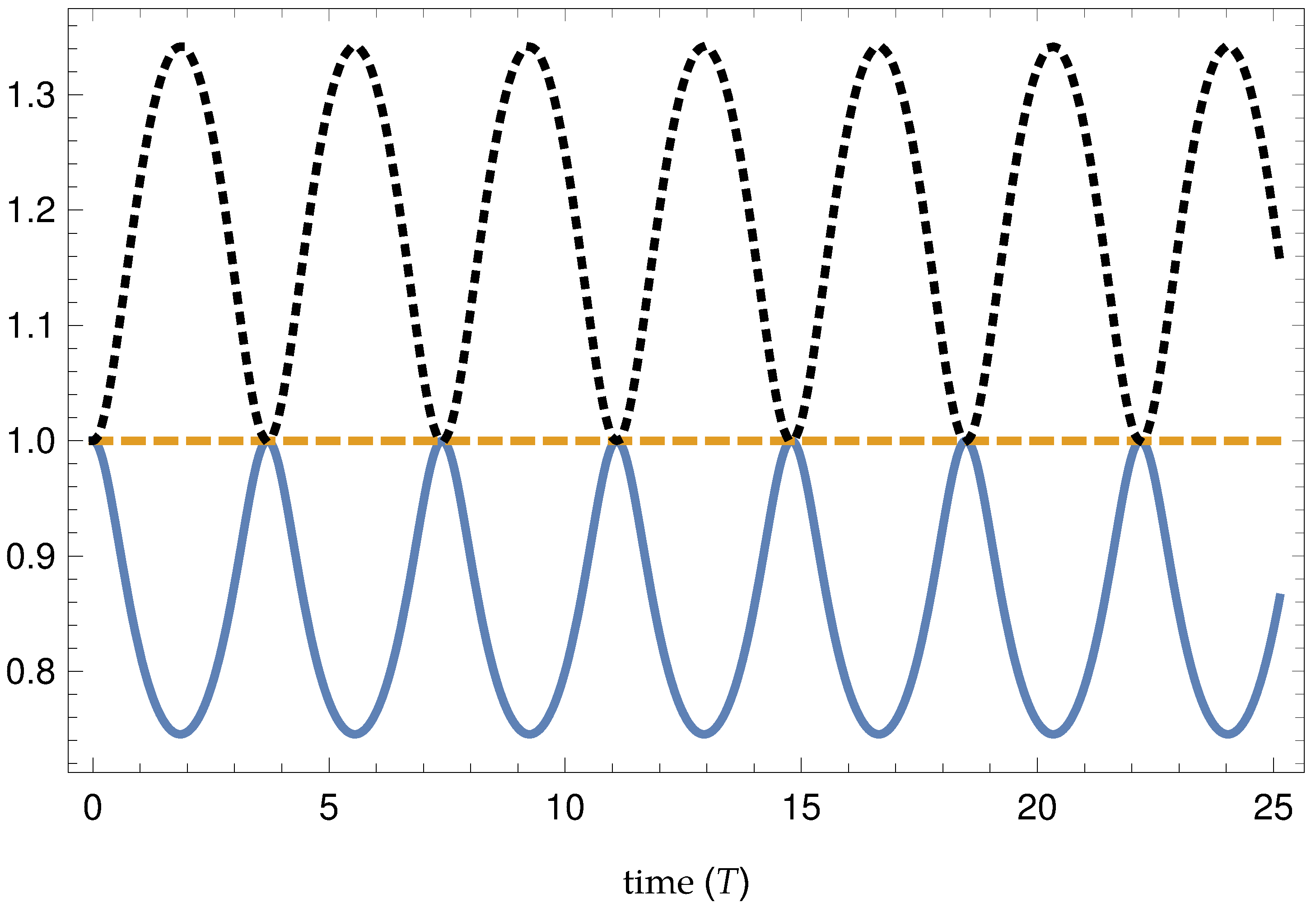
To make these conclusions more concrete, we plot angular speed, angular momentum, and energy as a function of time in Figure 2 for a specific choice of parameters. The equation of motion is complicated, but lends itself well to numerical solution. For definiteness and simplicity in this example, we consider the case of $c_{xx}=0.4$ with all other components of $c_{jk}$ being zero. This large but still perturbative value for $c_{jk}$ provides easily visible results in the plot. Calling the initial angular speed ${\omega }_0$, we plot the dimensionless angular speed $\Omega =\frac{\dot{\theta }}{{\omega }_0}$, the dimensionless energy $E=\frac{L}{m{l}^2{\omega }_0^2}$, and the dimensionless angular momentum $P_{\theta }=\frac{p_{\theta }}{2m{l}^2{\omega }_0}$ vs. the dimensionless time $T={\omega }_{0}t$ for the initial conditions $\theta \left(0\right)=0$, $\Omega \left(0\right)=1$. In conventional physics, the skaters pull their arms closer to the axis of rotation to increase their angular speed and extend their arms to slow their angular speed. Here, we see the perhaps entertaining result that when rotation invariance is violated in this way, the angular speed of the skater varies periodically without changes in the skater’s body configuration. We also see explicitly that energy is conserved while angular momentum is not. An animation of these results can be found at https://people.carleton.edu/~jtasson/animations.html.

6. Conclusions

In this work, we introduced an extension to Newton’s second law that permits a generic anisotropic mass. We discussed the use of this model in demonstrating foundational ideas in theoretical physics, and we develop its connection with contemporary efforts to test Lorentz symmetry in the context of the general test framework provided by the SME. We solved the block on the inclined plane as an example to make the ideas concrete and the spinning dumbbell as an illustration of the connection between symmetries and conservation laws. The material presented is useful in teaching theoretical physics ideas in classical mechanics and as an introduction to contemporary efforts to test spacetime symmetries.

References

1. Colladay, D.; Kostelecký, V.A. Lorentz-violating extension of the Standard Model. Phys. Rev. D 1998, 58, 116002. [Google Scholar] [CrossRef]
2. Kostelecký, V.A. Gravity, Lorentz violation, and the Standard Model. Phys. Rev. D 2004, 69, 105009. [Google Scholar] [CrossRef]
3. Tasson, J.D. What do we know about Lorentz invariance? Rep. Prog. Phys. 2014, 77, 062901. [Google Scholar] [CrossRef] [PubMed] [Green Version]
4. Kostelecký, V.A.; Russell, N. Data tables for Lorentz and CPT violation. Rev. Mod. Phys. 2011, 83, 11. [Google Scholar] [CrossRef]
5. Kostelecký, V.A.; Samuel, S. Spontaneous breaking of Lorentz symmetry in string theory. Phys. Rev. D 1989, 39, 683. [Google Scholar] [CrossRef]
6. Kostelecký, V.A.; Potting, R. CPT and strings. Nucl. Phys. B 1991, 359, 545. [Google Scholar] [CrossRef]
7. Wilczek, F. Whence the Force of F = ma? I: Culture Shock. Phys. Today 2004, 57, 11. [Google Scholar] [CrossRef]
8. Saslow, W.M. Accurate physical laws can permit new standard units: The two laws F = m a and the proportionality of weight to mass. Am. J. Phys. 2014, 82, 349. [Google Scholar] [CrossRef]
9. Goldstein, H.; Safko, J.L.; Poole, C.P. Classical Mechanics; Pearson: Essex, UK, 2014. [Google Scholar]
10. Taylor, J.R. Classical Mechanics; University Science Books: Sausalito, CA, USA, 2005. [Google Scholar]
11. Ciftja, O.; Livingston, V.; Thomas, E. Cyclotron motion of a charged particle with anisotropic mass. Am. J. Phys. 2017, 85, 359. [Google Scholar] [CrossRef]
12. Kostelecký, V.A.; Bluhm, R. Spontaneous Lorentz Violation, Nambu-Goldstone Modes, and Gravity. Phys. Rev. D 2005, 71, 065008. [Google Scholar]
13. Pruttivarasin, T.; Ramm, M.; Porsev, S.G.; Tupitsyn, I.I.; Safronova, M.; Hohensee, M.A.; Haeffner, H. A Michelson-Morley test of Lorentz symmetry for electrons. Nature 2015, 517, 592. [Google Scholar] [CrossRef] [PubMed]
14. Hohensee, M.A.; Leefer, N.; Budker, D.; Harabati, C.; Dzuba, V.A.; Flambaum, V.V. Limits on violations of Lorentz symmetry and the Einstein equivalence principle using radio-frequency spectroscopy of atomic dysprosium. Phys. Rev. Lett. 2013, 111, 050401. [Google Scholar] [CrossRef] [PubMed]
15. Smiciklas, M.; Brown, J.M.; Cheuk, L.W.; Romalis, M.V. A new test of local Lorentz invariance using 21Ne-Rb-K comagnetometer. Phys. Rev. Lett. 2011, 107, 171604. [Google Scholar] [CrossRef]
16. Flambaum, V.V.; Romalis, M.V. Effects of the Lorentz invariance violation in Coulomb interaction in nuclei and atoms. Phys. Rev. Lett. 2017, 118, 142501. [Google Scholar] [CrossRef] [PubMed]
17. Kostelecký, V.A.; Lane, C. Constraints on Lorentz violation from clock-comparison experiments. Phys. Rev. D 1999, 60, 116010. [Google Scholar] [CrossRef]
18. Altschul, B. Disentangling forms of Lorentz violation with complementary clock comparison experiments. Phys. Rev. D 2009, 79, 061702. [Google Scholar] [CrossRef]
19. Kostelecký, V.A.; Vargas, A. Lorentz and CPT tests with clock-comparison experiments. Phys. Rev. D 2018, 98, 036003. [Google Scholar] [CrossRef]
20. Lane, C. Using comparisons of clock frequencies and sidereal variation to probe Lorentz violation. Symmetry 2017, 9, 245. [Google Scholar] [CrossRef]
21. Bertschinger, T.H.; Flowers, N.A.; Tasson, J.D. Observer and particle transformations. In CPT and Lorentz Symmetry; Kostelecký, V.A., Ed.; World Scientific: Singapore, 2014; Volume VI. [Google Scholar]
22. Nobili, A.M.; Lucchesi, D.M.; Crosta, M.T.; Shao, M.; Turyshev, S.G.; Peron, R.; Catastini, G.; Anselmi, A.; Zavattini, G. On the universality of free fall, the equivalence principle, and the gravitational redshift. Am. J. Phys. 2015, 83, 39. [Google Scholar] [CrossRef]
23. Kostelecký, V.A.; Tasson, J.D. Matter-gravity couplings and Lorentz violation. Phys. Rev. D 2011, 83, 016013. [Google Scholar] [CrossRef]
24. Touboul, P.; Métris, G.; Rodrigues, M.; André, Y.; Baghi, Q.; Bergé, J.; Boulanger, D.; Bremer, S.; Carle, P.; Chhun, R.; et al. MICROSCOPE Mission: First Results of a Space Test of the Equivalence Principle. Phys. Rev. Lett. 2017, 119, 231101. [Google Scholar] [CrossRef] [PubMed]
25. Bailey, Q.G.; Kostelecký, V.A. Signals for Lorentz violation in post-newtonian gravity. Phys. Rev. D 2006, 74, 045001. [Google Scholar] [CrossRef]
26. Abbott, B.P.; Abbott, R.; Abbott, T.D.; Acernese, R.; Ackley, K.; Adams, C.; Adams, T.; Addesso, P.; Adhikari, R.X.; Adya, V.B.; et al. Gravitational waves and gamma-rays from a binary Neutron star merger: GW170817 and GRB 170817A. Astrophys. J. Lett. 2017, 848, L13. [Google Scholar] [CrossRef]
27. Neuenschwander, D.E. Resource Letter NTUC-1: Noether’s Theorem in the undergraduate curriculum. Am. J. Phys. 2014, 82, 183. [Google Scholar] [CrossRef]
28. Prigo, R.B.; Reading, M. Quantitative angular momentum experiment on the rotating chair. Am. J. Phys. 1977, 45, 636. [Google Scholar] [CrossRef]
29. Tasson, J.D. Antimatter, Lorentz symmetry, and gravity. JPS Conf. Proc. 2017, 18, 011002. [Google Scholar]
30. Kostelecký, V.A.; Mewes, M. Fermions with Lorentz-violating operators of arbitrary dimension. Phys. Rev. D 2013, 88, 096006. [Google Scholar] [CrossRef]
31. Kostelecký, V.A.; Mewes, M. Electrodynamics with Lorentz-violating operators of arbitrary dimension. Phys. Rev. D 2009, 80, 015020. [Google Scholar] [CrossRef]
32. Kostelecký, V.A.; Mewes, M. Testing local Lorentz invariance with gravitational waves. Phys. Lett. B 2016, 757, 510. [Google Scholar] [CrossRef]
33. Tasson, J.D. Lorentz violation, gravitomagnetism, and intrinsic spin. Phys. Rev. D 2012, 86, 124021. [Google Scholar] [CrossRef]
34. Kostelecký, V.A.; Russell, N.; Tasson, J.D. Constraints on torsion from bounds on Lorentz violation. Phys. Rev. Lett. 2008, 100, 111102. [Google Scholar] [CrossRef] [PubMed]
35. Foster, J.; Kostelecký, V.A.; Xu, R. Constraints on nonmetricity from bounds on Lorentz violation. Phys. Rev. D 2017, 95, 084033. [Google Scholar] [CrossRef] [Green Version]
36. Kostelecký, V.A.; Russell, N. Classical kinematics for Lorentz violation. Phys. Lett. B 2010, 693, 443. [Google Scholar] [CrossRef]
37. Kostelecký, V.A. Riemann-Finsler geometry and Lorentz-violating kinematics. Phys. Lett. B 2011, 701, 137. [Google Scholar] [CrossRef]
38. Foster, J.; Lehnert, R. Classical-physics applications for Finsler b space. Phys. Lett. B 2015, 746, 164. [Google Scholar] [CrossRef]
Figure 1. Block on an inclined plane with gravitational field g and background field c j k : (left) the systemwith the original coordinates (unprimed) and the observer-rotated coordinates (primed); (right) the particle rotated system with the original coordinates. In each case, g points toward the center of the Earth.
Symmetry 11 00022 g001
Figure 2. Rigid rotor results vs. dimensionless time: dimensionless angular speed (solid), dimensionless energy (dashed), dimensionless angular momentum (dotted).
Symmetry 11 00022 g002