New Exact Solutions of the Generalized Benjamin–Bona–Mahony Equation

Abstract

The recently introduced technique, namely the generalized exponential rational function method, is applied to acquire some new exact optical solitons for the generalized Benjamin–Bona–Mahony (GBBM) equation. Appropriately, we obtain many families of solutions for the considered equation. To better understand of the physical features of solutions, some physical interpretations of solutions are also included. We examined the symmetries of obtained solitary waves solutions through figures. It is concluded that our approach is very efficient and powerful for integrating different nonlinear pdes. All symbolic computations are performed in Maple package.

1. Introduction

The Benjamin–Bona–Mahony (BBM) equation has been studied by Benjamin, Bona, and Mahony in 1972 as the improved KdV equation for the description of long surface gravity waves having a small amplitude. They have also investigated the stability and uniqueness of solutions to the BBM equation [1]. The description of the drift of waves in plasma physics, the propagation of wave in semi-conductors and optical devices [2], and the behavior of Rossby waves in rotating fluids [3] are some other phenomena that are modeled by this equation.

Let us consider the dimensionless form of the (1 + 1) the generalized Benjamin–Bona–Mahony (GBBM) equation as follows [4]:

$$\begin{array}{c}\hfill u_t+\alpha u_x+(\beta u^{\vartheta }+\gamma u^{2\vartheta })u_x-\delta u_{xxt}=0,\end{array}$$

(1)

with the unknown function u and the constants of $\alpha$, $\delta$, n, $\beta$ and $\vartheta$.

It is also known that the multi-soliton solutions for the Equation (1) only exist with the conditions $\gamma =0$ and $\vartheta =1$, i.e., whenever we have

$$\begin{array}{c}\hfill u_t+\alpha u_x+\left(\beta u\right)u_x-\delta u_{xxt}=0.\end{array}$$

(2)

The main application of the BBM equation is related to model the hydromagnetic waves in cold plasma, the acoustic waves in anharmonic crystals and the acoustic-gravity waves in compressible fluids [5,6].

Recently, the investigation of exact solutions of nonlinear PDEs has begun to attract mathematicians and physicists’ attention because of the onset of soliton [7,8,9]. Therefore, several efficient techniques for handling NPDEs have been developed. Among them, we can list the traditional methods: the Hirotas bilinear method [10] and the Darboux transformation method [11]. There are also some recent direct and algebraic methods: the variational iteration method [12], the exp-function method [13], various extended tanh-function methods [14] and Lie symmetry analysis [15,16,17].

The relatively new technique called the generalized exponential rational function method (or GERFM in short) was firstly suggested by Ghanbari et al. in Ref. [18] to solve the resonance nonlinear Schrödinger equation as

$$i{\psi }_t+\alpha {\psi }_{xx}+\beta \mathcal{F}\left({\left|\psi \right|}^2\right)\psi +\gamma \left(\frac{{\left|\psi \right|}_{xx}}{\left|\psi \right|}\right)\psi =0,i=\sqrt{-1}.$$

(3)

Another application of the method has been carried out in Ref. [19] where the authors have implemented the method to solve the Fokas–Lenells equation in the presence of the perturbation terms, as follows:

$$i\frac{\partial \psi }{\partial t}+\frac{{\partial }^2\psi }{\partial x^2}+\alpha {\left|\psi \right|}^2\psi +i\left[{\gamma }_1\frac{\partial {\psi }^3}{\partial x^3}+{\gamma }_2\frac{\partial \psi }{\partial x}{\left|\psi \right|}^2+{\gamma }_3\frac{{\partial \left|\psi \right|}^2}{\partial x}\psi \right]=0.$$

(4)

The method also has been successfully implemented to retrieve traveling wave solutions to the nonlinear Schrödinger’s equation in the presence of Hamiltonian perturbations [20] as

$$i{\psi }_t+a{\psi }_{xx}+\left(b_1\left|\psi \right|+b_2{\left|\psi \right|}^2\right)\psi =i\{\alpha {\psi }_x+\lambda {\left({\left|\psi \right|}^2\psi \right)}_x+\theta {\left({\left|\psi \right|}^2\right)}_x\psi \}.$$

(5)

In all cases, the authors have declared that the method introduces some new solutions that have not been reported in previous works. In addition, it deduces that the method can be applied to study many other nonlinear PDEs in many branches of physics, biology, engineering. This research aims to integrate the GBBM Equation (1) using the GERFM. For this reason, our paper is organized as below: Section 2 deals with the presentation of the method. Section 3 is devoted to the application of GERFM to the GBBM equation. Eventually, the conclusion of the present research is outlined in the last section.

2. The Main Steps of GERFM

In this subsection, we review the routine description of GERFM.

• Let us take into account the nonlinear PDE in the form:

  $$\mathcal{L}(\psi ,{\psi }_x,{\psi }_t,{\psi }_{xx},\dots )=0.$$

  (6)
  Using the transformations $\psi =\psi \left(\eta \right)$ and $\eta =\sigma x-lt$, Equation (6) is reduced to following NODE as:

  $$\mathcal{L}(\psi ,{\psi }^{\prime },{\psi }^{″},\dots )=0,$$

  (7)

  where the values of $\sigma$ and l will be found later.
• Now, the structure of the wave solution of Equation (7) is assumed to be

  $$\psi \left(\eta \right)=p_0+\sum _{k=1}^M{p}_k\mathsf{\Theta }{\left(\eta \right)}^k+\sum _{k=1}^M\frac{q_k}{\mathsf{\Theta }{\left(\eta \right)}^k},$$

  (8)

  where

  $$\mathsf{\Theta }\left(\eta \right)=\frac{{\iota }_1{e}^{{\kappa }_1\eta }+{\iota }_2{e}^{{\kappa }_2\eta }}{{\iota }_3{e}^{{\kappa }_3\eta }+{\iota }_4{e}^{{\kappa }_4\eta }}.$$

  (9)
  The values of constants ${\iota }_i,{\kappa }_i(1\le i\le 4)$, $p_0,p_k$ and $q_k(1\le k\le M)$ are determined, in such a way that solution (8) always persuade Equation (7). By considering the homogenous balance principle, the value of M is determined.
• Substituting Equation (8) into Equation (7), an algebraic equation $P(S_1,S_2,S_3,S_4)=0$ in terms of $S_i=e^{q_i\eta }$ for $i=1,\dots ,4$ is constructed. Then, making each coefficient for the powers of P to zero, we acquire a series of nonlinear equations in terms of $p_i,q_i(1\le i\le 4)$, and $\sigma ,l,p_0,p_k$ and $q_k(1\le k\le M)$ is generated.
• By solving the above system of equations using any computer package like Maple (18, Waterloo Maple, Canada), the values of ${\iota }_i,{\kappa }_i(1\le i\le 4)$, $p_0,p_k$, and $q_k(1\le k\le M)$ are determined, replacing these values in Equation (8) provides us the exact solutions of the nonlinear PDE (6).

3. Utilization of GERFM for the GBBM Equation

Let us consider the following dependent variable transformation

$$u\left(x,t\right)=\psi \left(\eta \right),\eta =kx-\theta t,$$

(10)

where k and $\theta$ are constants need to be calculated. Under the transformation of Equation (10), Equation (1) can be reduced to the following NODE:

$$\left(\alpha k-\theta \right){\psi }_{\eta }+k\left(\beta {\psi }^{\vartheta }+\gamma {\psi }^{2\vartheta }\right){\psi }_{\eta }+\delta k^2\theta {\psi }_{\eta \eta \eta }=0.$$

(11)

We may now integrate Equation (11) to have

$$\left(\alpha k-\theta \right)\psi +k\left(\frac{\beta }{\vartheta +1}{\psi }^{\vartheta +1}+\frac{\gamma }{2\vartheta +1}{\psi }^{2\vartheta +1}\right)+\delta k^2\theta {\psi }_{\eta \eta }=0.$$

(12)

Using the transformation $\psi ={\psi }^n$ in (12), we attain

$$\psi {\psi }_{\eta \eta }+{\sigma }_1{\psi }^2+{\sigma }_2{\psi }^3+{\sigma }_3{\psi }^4+{\sigma }_4{\left({\psi }_{\eta }\right)}^2=0,$$

(13)

where

$$\begin{array}{ccc}\hfill {\sigma }_1& =& \frac{\left(\alpha k-\theta \right)\vartheta }{\delta k^2\theta },\hfill \\ \hfill {\sigma }_2& =& \frac{\beta \vartheta }{\delta k(\vartheta +1)\theta },\hfill \\ \hfill {\sigma }_3& =& \frac{\gamma \vartheta }{\delta k(2\vartheta +1)\theta },\hfill \\ \hfill {\sigma }_4& =& \frac{1-\vartheta }{\vartheta }.\hfill \end{array}$$

In this section, GERFM will be used to determine solitary wave solutions of (1). To this end, if we apply the balancing principle for the terms of ${\psi }^4$ and ${\left({\psi }_{\eta }\right)}^2$ in (13), (i.e., $4M=2(M+1)$), we get $M=1$. This implies that Equation (1) has the solution given by

$$\psi \left(\eta \right)=p_0+p_1\mathsf{\Theta }\left(\eta \right)+\frac{q_1}{\mathsf{\Theta }\left(\eta \right)}.$$

(14)

We now exert the GERFM to derive the following categories of solutions for Equation (1):

Family 1:

We attain $\iota =[1,1,1,-1]$ and $\kappa =[1,-1,1,-1]$, so we will obtain

$$\mathsf{\Theta }\left(\eta \right)=\frac{-3-2{\mathrm{e}}^{\eta }}{1+{\mathrm{e}}^{\eta }}.$$

(15)

Case 1:

$$\theta =-\frac{\sqrt{2\vartheta +1}\sqrt{\left(\gamma \vartheta +\gamma \right){\left(\vartheta +2\right)}^2\alpha -\left(2\vartheta +1\right){\beta }^2}\vartheta \beta }{\sqrt{-\delta }\left(\gamma \vartheta +\gamma \right){\left(\vartheta +2\right)}^2},$$

$$k=-\frac{\sqrt{2\vartheta +1}\vartheta \beta }{\sqrt{-\delta }\sqrt{\left(\gamma \vartheta +\gamma \right){\left(\vartheta +2\right)}^2\alpha -\left(2\vartheta +1\right){\beta }^2}},$$

$$p_0=\frac{\left(-6\vartheta -3\right)\beta }{\gamma \left(\vartheta +2\right)},p_1=0,q_1=\frac{\left(-12n-6\right)\beta }{\gamma \left(\vartheta +2\right)}.$$

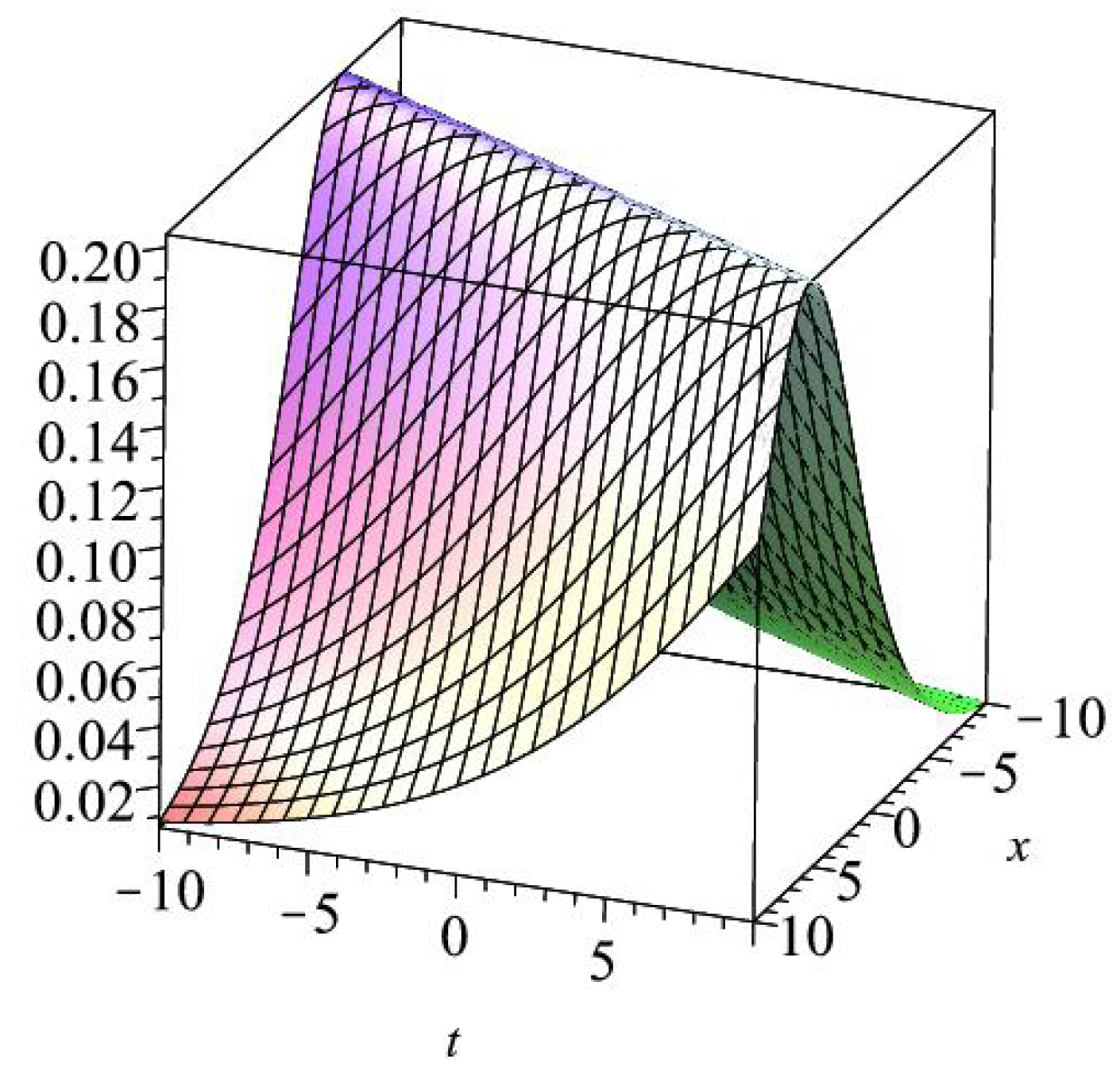
These resulting values direct us to have

$$\psi \left(\eta \right)=\frac{\left(-6\vartheta -3\right)\beta }{\gamma \left(\vartheta +2\right)\left(3+2{\mathrm{e}}^{\eta }\right)}.$$

Consequently, we can get the following exact wave solution

$$u_1\left(x,t\right)={\left(\frac{\left(-6\vartheta -3\right)\beta }{\gamma \left(\vartheta +2\right)\left(3+2{\mathrm{e}}^{\eta }\right)}\right)}^{\frac{1}{\vartheta }},$$

(16)

where

$$\eta =-\frac{\sqrt{2\vartheta +1}\vartheta \beta }{\sqrt{-\delta }\sqrt{\left(\gamma \vartheta +\gamma \right){\left(\vartheta +2\right)}^2\alpha -\left(2\vartheta +1\right){\beta }^2}}x+$$

$$\frac{\sqrt{2\vartheta +1}\sqrt{\left(\gamma \vartheta +\gamma \right){\left(\vartheta +2\right)}^2\alpha -\left(2\vartheta +1\right){\beta }^2}\vartheta \beta }{\sqrt{-\delta }\left(\gamma \vartheta +\gamma \right){\left(\vartheta +2\right)}^2}t.$$

Case 2:

$$\theta =-\frac{\sqrt{2\vartheta +1}\sqrt{25\left(\gamma \vartheta +\gamma \right){\left(\vartheta +2\right)}^2\alpha -\left(2\vartheta +1\right){\beta }^2}\vartheta \beta }{25\sqrt{-\delta }\left(\gamma \vartheta +\gamma \right){\left(\vartheta +2\right)}^2},$$

$$k=-\frac{\sqrt{2\vartheta +1}\vartheta \beta }{\sqrt{-\delta }\sqrt{25\left(\gamma \vartheta +\gamma \right){\left(\vartheta +2\right)}^2\alpha -\left(2\vartheta +1\right){\beta }^2}},$$

$$p_0=\frac{\left(-2n-1\right)\beta }{\gamma \left(\vartheta +2\right)},p_1=-\frac{\beta \left(2\vartheta +1\right)}{5\gamma \left(\vartheta +2\right)},q_1=-\frac{6\beta \left(2\vartheta +1\right)}{5\gamma \left(\vartheta +2\right)}$$

led

$$\psi \left(\eta \right)=\frac{\left(-2\vartheta -1\right)\beta {\mathrm{e}}^{\eta }}{\left(\vartheta +2\right)\left(1+{\mathrm{e}}^{\eta }\right)\gamma \left(15+10{\mathrm{e}}^{\eta }\right)}.$$

Hence, we get the following solitary wave solution for GBBM as

$$u_2\left(x,t\right)={\left(\frac{\left(-2\vartheta -1\right)\beta {\mathrm{e}}^{\eta }}{\left(\vartheta +2\right)\left(1+{\mathrm{e}}^{\eta }\right)\gamma \left(15+10{\mathrm{e}}^{\eta }\right)}\right)}^{\frac{1}{\vartheta }},$$

(17)

where

$$\eta =-\frac{\sqrt{2\vartheta +1}\vartheta \beta }{\sqrt{-\delta }\sqrt{25\left(\gamma \vartheta +\gamma \right){\left(\vartheta +2\right)}^2\alpha -\left(2\vartheta +1\right){\beta }^2}}x+$$

$$\frac{\sqrt{2\vartheta +1}\sqrt{25\left(\gamma \vartheta +\gamma \right){\left(\vartheta +2\right)}^2\alpha -\left(2\vartheta +1\right){\beta }^2}\vartheta \beta }{25\sqrt{-\delta }\left(\gamma \vartheta +\gamma \right){\left(\vartheta +2\right)}^2}t.$$

Family 2:

We attain $\iota =[1,1,1,-1]$ and $\kappa =[1,-1,1,-1]$, so we will obtain

$$\mathsf{\Theta }\left(\eta \right)=-\frac{sin\left(\eta \right)}{cos\left(\eta \right)}.$$

(18)

Case 1:

$$\theta =\frac{\sqrt{2\vartheta +1}\sqrt{\left(\gamma \vartheta +\gamma \right){\left(\vartheta +2\right)}^2\alpha -\left(2\vartheta +1\right){\beta }^2}\vartheta \beta }{2\sqrt{\delta }\left(\gamma \vartheta +\gamma \right){\left(\vartheta +2\right)}^2},$$

$$k=\frac{\sqrt{2\vartheta +1}\vartheta \beta }{2\sqrt{\delta }\sqrt{\left(\gamma \vartheta +\gamma \right){\left(\vartheta +2\right)}^2\alpha -\left(2\vartheta +1\right){\beta }^2}},$$

$$p_0=-\frac{\beta \left(2\vartheta +1\right)}{2\gamma \left(\vartheta +2\right)},p_1=0,q_1=\frac{i\left(2\vartheta +1\right)\beta }{2\gamma \left(\vartheta +2\right)}.$$

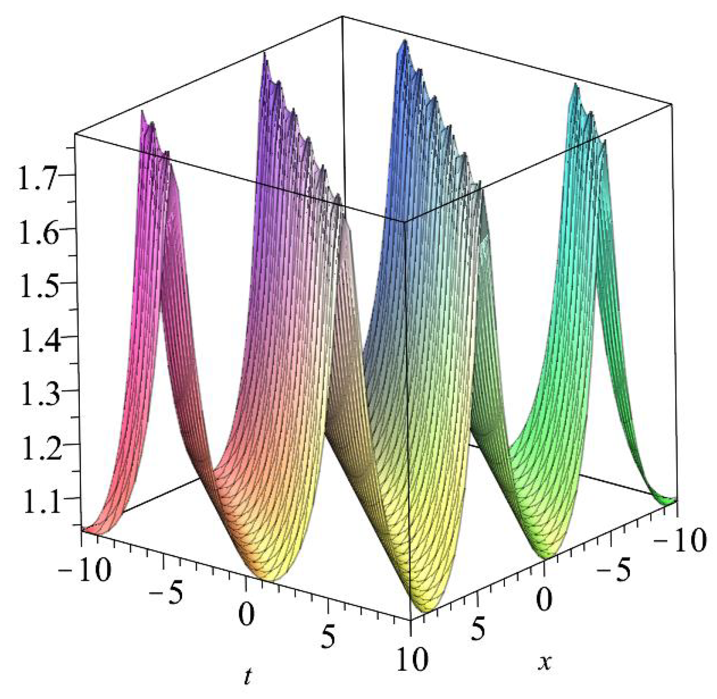
These resulting values help us to have

$$\psi \left(\eta \right)=-\frac{ksinh\left(\eta \right)}{\sqrt{2{\gamma }^2{k}^2-{\gamma }^2{q}^2+2q\gamma -1}\sqrt{\vartheta }cosh\left(\eta \right)}.$$

Consequently, the following exact wave solution is determined

$$u_3\left(x,t\right)={\left(-\frac{ksinh\left(\eta \right)}{\sqrt{2{\gamma }^2{k}^2-{\gamma }^2{q}^2+2q\gamma -1}\sqrt{\vartheta }cosh\left(\eta \right)}\right)}^{\frac{1}{\vartheta }},$$

(19)

where

$$\eta =\frac{\sqrt{2\vartheta +1}\vartheta \beta }{2\sqrt{\delta }\sqrt{\left(\gamma \vartheta +\gamma \right){\left(\vartheta +2\right)}^2\alpha -\left(2\vartheta +1\right){\beta }^2}}x-$$

$$\frac{\sqrt{2\vartheta +1}\sqrt{\left(\gamma \vartheta +\gamma \right){\left(\vartheta +2\right)}^2\alpha -\left(2\vartheta +1\right){\beta }^2}\vartheta \beta }{2\sqrt{\delta }\left(\gamma \vartheta +\gamma \right){\left(\vartheta +2\right)}^2}t.$$

Family 3:

We attain $\iota =[1,1,1,-1]$ and $\kappa =[1,-1,1,-1]$, so we will obtain

$$\mathsf{\Theta }\left(\eta \right)=\frac{sin\left(\eta \right)+cos\left(\eta \right)}{cos\left(\eta \right)}.$$

(20)

Case 1:

$$\theta =-\frac{\sqrt{2\vartheta +1}\sqrt{\left(\gamma \vartheta +\gamma \right){\left(\vartheta +2\right)}^2\alpha +\left(2\vartheta +1\right){\beta }^2}\vartheta \beta }{\sqrt{-\delta }\left(\gamma \vartheta +\gamma \right){\left(\vartheta +2\right)}^2},$$

$$k=-\frac{\sqrt{2\vartheta +1}\vartheta \beta }{\sqrt{-\delta }\sqrt{\left(\gamma \vartheta +\gamma \right){\left(\vartheta +2\right)}^2\alpha +\left(2\vartheta +1\right){\beta }^2}},$$

$$p_0=\frac{\left(-2\vartheta -1\right)\beta }{\gamma \left(\vartheta +2\right)},p_1=\frac{\beta \left(2\vartheta +1\right)}{2\gamma \left(\vartheta +2\right)},q_1=\frac{\beta \left(2\vartheta +1\right)}{\gamma \left(\vartheta +2\right)}.$$

These resulting values led us to obtain

$$\psi \left(\eta \right)=\frac{\beta \left(2\vartheta +1\right)}{2\left(\vartheta +2\right)\gamma cos\left(\eta \right)\left(sin\left(\eta \right)+cos\left(\eta \right)\right)}.$$

Hence, one arrives to the following exact wave solution:

$$u_4\left(x,t\right)={\left(\frac{\beta \left(2\vartheta +1\right)}{2\left(\vartheta +2\right)\gamma cos\left(\eta \right)\left(sin\left(\eta \right)+cos\left(\eta \right)\right)}\right)}^{\frac{1}{\vartheta }},$$

(21)

where

$$\eta =-\frac{\sqrt{2\vartheta +1}\vartheta \beta }{\sqrt{-\delta }\sqrt{\left(\gamma \vartheta +\gamma \right){\left(\vartheta +2\right)}^2\alpha +\left(2\vartheta +1\right){\beta }^2}}x+$$

$$\frac{\sqrt{2\vartheta +1}\sqrt{\left(\gamma \vartheta +\gamma \right){\left(\vartheta +2\right)}^2\alpha +\left(2\vartheta +1\right){\beta }^2}\vartheta \beta }{\sqrt{-\delta }\left(\gamma \vartheta +\gamma \right){\left(\vartheta +2\right)}^2}t.$$

Family 4:

We attain $\iota =[1,1,1,-1]$ and $\kappa =[1,-1,1,-1]$, so we will obtain

$$\mathsf{\Theta }\left(\eta \right)=\frac{-sin\left(\eta \right)+cos\left(\eta \right)}{sin\left(\eta \right)}.$$

(22)

Case 1:

$$\theta =-\frac{\sqrt{2\vartheta +1}\sqrt{\left(\gamma \vartheta +\gamma \right){\left(\vartheta +2\right)}^2\alpha +\left(2\vartheta +1\right){\beta }^2}\vartheta \beta }{2\sqrt{-\delta }\left(\gamma \vartheta +\gamma \right){\left(\vartheta +2\right)}^2},$$

$$k=-\frac{\sqrt{2\vartheta +1}\vartheta \beta }{2\sqrt{-\delta }\sqrt{\left(\gamma \vartheta +\gamma \right){\left(\vartheta +2\right)}^2\alpha +\left(2\vartheta +1\right){\beta }^2}},$$

$$p_0=\frac{\left(-2\vartheta -1\right)\beta }{\gamma \left(\vartheta +2\right)},p_1=-\frac{\beta \left(2\vartheta +1\right)}{2\gamma \left(\vartheta +2\right)},q_1=\frac{\left(-2\vartheta -1\right)\beta }{\gamma \left(\vartheta +2\right)}.$$

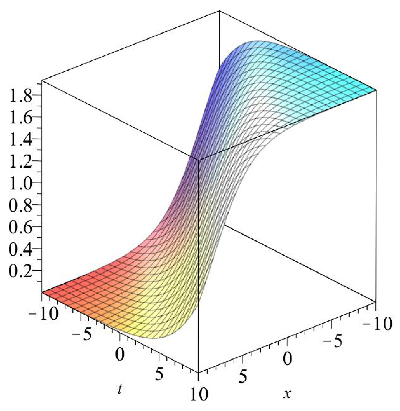
These solutions direct us to get

$$\psi \left(\eta \right)=\frac{\beta \left(2\vartheta +1\right)}{2\gamma \left(\vartheta +2\right)sin\left(\eta \right)\left(sin\left(\eta \right)-cos\left(\eta \right)\right)}.$$

As a result, we can get the following exact wave solution:

$$u_5\left(x,t\right)={\left(\frac{\beta \left(2\vartheta +1\right)}{2\gamma \left(\vartheta +2\right)sin\left(\eta \right)\left(sin\left(\eta \right)-cos\left(\eta \right)\right)}\right)}^{\frac{1}{\vartheta }},$$

(23)

where

$$\eta =-\frac{\sqrt{2\vartheta +1}\vartheta \beta }{2\sqrt{-\delta }\sqrt{\left(\gamma \vartheta +\gamma \right){\left(\vartheta +2\right)}^2\alpha +\left(2\vartheta +1\right){\beta }^2}}x+$$

$$\frac{\sqrt{2\vartheta +1}\sqrt{\left(\gamma \vartheta +\gamma \right){\left(\vartheta +2\right)}^2\alpha +\left(2\vartheta +1\right){\beta }^2}\vartheta \beta }{2\sqrt{-\delta }\left(\gamma \vartheta +\gamma \right){\left(\vartheta +2\right)}^2}t.$$

Family 5:

We attain $\iota =[1,1,1,-1]$ and $\kappa =[1,-1,1,-1]$, so we will obtain

$$\mathsf{\Theta }\left(\eta \right)=-\frac{1}{1+{\mathrm{e}}^{\eta }}.$$

(24)

Case 1:

$$\theta =-\frac{\sqrt{2\vartheta +1}\sqrt{\left(\gamma \vartheta +\gamma \right){\left(\vartheta +2\right)}^2\alpha -\left(2\vartheta +1\right){\beta }^2}\vartheta \beta }{\sqrt{-\delta }\left(\gamma \vartheta +\gamma \right){\left(\vartheta +2\right)}^2},$$

$$k=-\frac{\sqrt{2\vartheta +1}\vartheta \beta }{\sqrt{-\delta }\sqrt{\left(\gamma \vartheta +\gamma \right){\left(\vartheta +2\right)}^2\alpha -\left(2\vartheta +1\right){\beta }^2}},$$

$$p_0=0,p_1=\frac{\beta \left(2\vartheta +1\right)}{\gamma \left(\vartheta +2\right)},q_1=0.$$

Then, we arrived to

$$\psi \left(\eta \right)=\frac{\left(-2\vartheta -1\right)\beta }{\gamma \left(\vartheta +2\right)\left(1+{\mathrm{e}}^{\eta }\right)}.$$

Therefore, the following exact wave solution for the equation is achieved

$$u_6\left(x,t\right)={\left(\frac{\left(-2\vartheta -1\right)\beta }{\gamma \left(\vartheta +2\right)\left(1+{\mathrm{e}}^{\eta }\right)}\right)}^{\frac{1}{\vartheta }},$$

(25)

where

$$\eta =-\frac{\sqrt{2\vartheta +1}\vartheta \beta }{\sqrt{-\delta }\sqrt{\left(\gamma \vartheta +\gamma \right){\left(\vartheta +2\right)}^2\alpha -\left(2\vartheta +1\right){\beta }^2}}x+$$

$$\frac{\sqrt{2\vartheta +1}\sqrt{\left(\gamma \vartheta +\gamma \right){\left(\vartheta +2\right)}^2\alpha -\left(2\vartheta +1\right){\beta }^2}\vartheta \beta }{\sqrt{-\delta }\left(\gamma \vartheta +\gamma \right){\left(\vartheta +2\right)}^2}t.$$

Family 6:

We attain $\iota =[1,1,1,-1]$ and $\kappa =[1,-1,1,-1]$, so we will obtain

$$\mathsf{\Theta }\left(\eta \right)=\frac{3{\mathrm{e}}^{\eta }+2}{1+{\mathrm{e}}^{\eta }}.$$

(26)

Case 1:

$$\theta =-\frac{\sqrt{2\vartheta +1}\sqrt{\left(\gamma \vartheta +\gamma \right){\left(\vartheta +2\right)}^2\alpha -\left(2\vartheta +1\right){\beta }^2}\vartheta \beta }{\sqrt{-\delta }\left(\gamma \vartheta +\gamma \right){\left(\vartheta +2\right)}^2},$$

$$k=-\frac{\sqrt{2\vartheta +1}\vartheta \beta }{\sqrt{-\delta }\sqrt{\left(\gamma \vartheta +\gamma \right){\left(\vartheta +2\right)}^2\alpha -\left(2\vartheta +1\right){\beta }^2}},$$

$$p_0=\frac{\left(-4n-2\right)\beta }{\gamma \left(\vartheta +2\right)},p_1=0,q_1=\frac{\left(-4n-2\right)\beta }{\gamma \left(\vartheta +2\right)}.$$

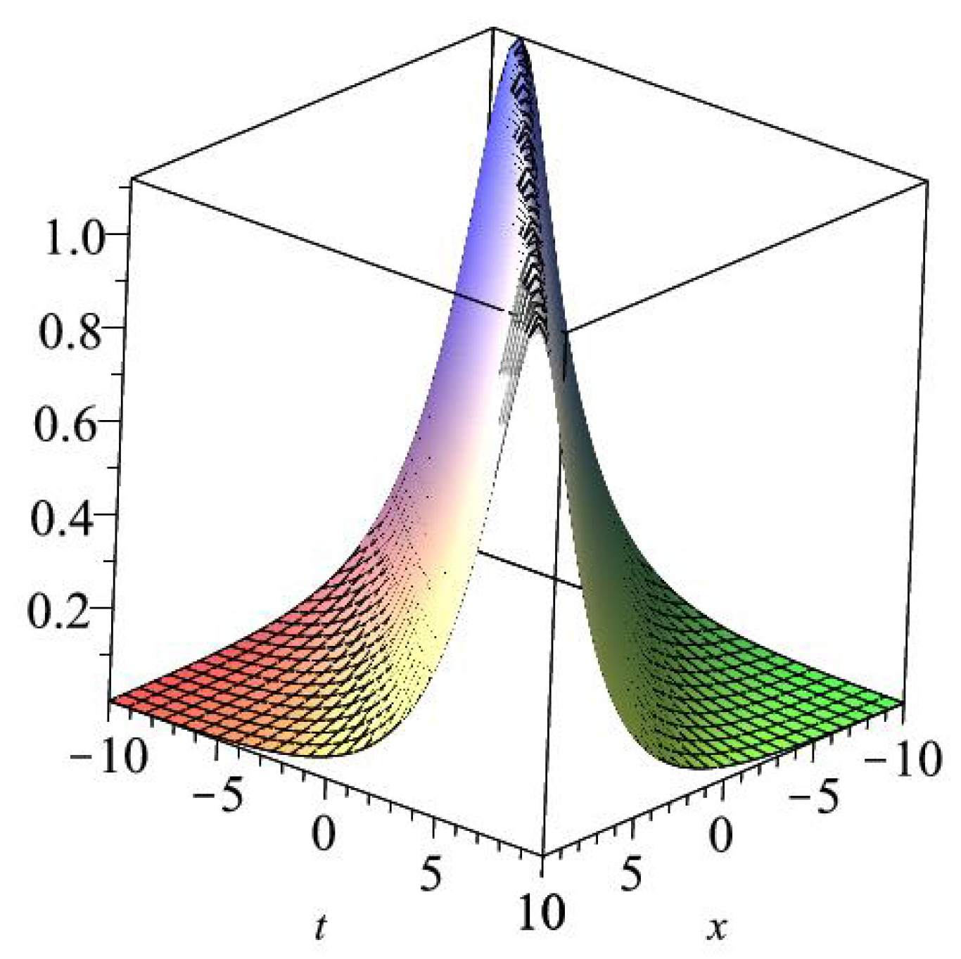
These values let us to consider

$$\psi \left(\eta \right)=\frac{\left(-4n-2\right)\beta }{\gamma \left(\vartheta +2\right)\left({\mathrm{e}}^{\eta }+2\right)}.$$

Thus, we obtain

$$u_7\left(x,t\right)={\left(\frac{\left(-4n-2\right)\beta }{\gamma \left(\vartheta +2\right)\left({\mathrm{e}}^{\eta }+2\right)}\right)}^{\frac{1}{\vartheta }},$$

(27)

where

$$\eta =-\frac{\sqrt{2\vartheta +1}\vartheta \beta }{\sqrt{-\delta }\sqrt{\left(\gamma \vartheta +\gamma \right){\left(\vartheta +2\right)}^2\alpha -\left(2\vartheta +1\right){\beta }^2}}x+$$

$$\frac{\sqrt{2\vartheta +1}\sqrt{\left(\gamma \vartheta +\gamma \right){\left(\vartheta +2\right)}^2\alpha -\left(2\vartheta +1\right){\beta }^2}\vartheta \beta }{\sqrt{-\delta }\left(\gamma \vartheta +\gamma \right){\left(\vartheta +2\right)}^2}t.$$

Family 7:

We attain $\iota =[1,1,1,-1]$ and $\kappa =[1,-1,1,-1]$, so we will obtain

$$\mathsf{\Theta }\left(\eta \right)=\frac{-{\mathrm{e}}^{\eta }-2}{1+{\mathrm{e}}^{\eta }}.$$

(28)

Case 1:

$$\theta =-\frac{\sqrt{2\vartheta +1}\sqrt{\left(\gamma \vartheta +\gamma \right){\left(\vartheta +2\right)}^2\alpha -\left(2\vartheta +1\right){\beta }^2}\vartheta \beta }{\sqrt{-\delta }\left(\gamma \vartheta +\gamma \right){\left(\vartheta +2\right)}^2},$$

$$k=-\frac{\sqrt{2\vartheta +1}\vartheta \beta }{\sqrt{-\delta }\sqrt{\left(\gamma \vartheta +\gamma \right){\left(\vartheta +2\right)}^2\alpha -\left(2\vartheta +1\right){\beta }^2}},$$

$$p_0=\frac{\left(-6\vartheta -3\right)\beta }{\gamma \left(\vartheta +2\right)},p_1=0,q_1=\frac{\left(12n+6\right)\beta }{\gamma \left(\vartheta +2\right)}.$$

These resulting values help us to consider

$$\psi \left(\eta \right)=\frac{\left(-6\vartheta -3\right)\beta {\mathrm{e}}^{\eta }}{\gamma \left(\vartheta +2\right)\left(3{\mathrm{e}}^{\eta }+2\right)}.$$

Accordingly, we can get the following exact wave solution

$$u_8\left(x,t\right)={\left(\frac{\left(-6\vartheta -3\right)\beta {\mathrm{e}}^{\eta }}{\gamma \left(\vartheta +2\right)\left(3{\mathrm{e}}^{\eta }+2\right)}\right)}^{\frac{1}{\vartheta }},$$

(29)

where

$$\eta =-\frac{\sqrt{2\vartheta +1}\vartheta \beta }{\sqrt{-\delta }\sqrt{\left(\gamma \vartheta +\gamma \right){\left(\vartheta +2\right)}^2\alpha -\left(2\vartheta +1\right){\beta }^2}}x+$$

$$\frac{\sqrt{2\vartheta +1}\sqrt{\left(\gamma \vartheta +\gamma \right){\left(\vartheta +2\right)}^2\alpha -\left(2\vartheta +1\right){\beta }^2}\vartheta \beta }{\sqrt{-\delta }\left(\gamma \vartheta +\gamma \right){\left(\vartheta +2\right)}^2}t.$$

Family 8:

We attain $\iota =[1,1,1,-1]$ and $\kappa =[1,-1,1,-1]$, so we will obtain

$$\mathsf{\Theta }\left(\eta \right)=\frac{2{\mathrm{e}}^{\eta }+1}{1+{\mathrm{e}}^{\eta }}.$$

(30)

Case 1:

$$\theta =-\frac{\sqrt{2\vartheta +1}\sqrt{9\left(\gamma \vartheta +\gamma \right){\left(\vartheta +2\right)}^2\alpha -\left(2\vartheta +1\right){\beta }^2}\vartheta \beta }{9\sqrt{-\delta }\left(\gamma \vartheta +\gamma \right){\left(\vartheta +2\right)}^2},$$

$$k=-\frac{\sqrt{2\vartheta +1}\vartheta \beta }{\sqrt{-\delta }\sqrt{9\left(\gamma \vartheta +\gamma \right){\left(\vartheta +2\right)}^2\alpha -\left(2\vartheta +1\right){\beta }^2}},$$

$$p_0=\frac{\left(-2\vartheta -1\right)\beta }{\gamma \left(\vartheta +2\right)},p_1=\frac{\beta \left(2\vartheta +1\right)}{3\gamma \left(\vartheta +2\right)},q_1=\frac{2\beta \left(2\vartheta +1\right)}{3\gamma \left(\vartheta +2\right)}.$$

From these results, one has

$$\psi \left(\eta \right)=\frac{\left(-2\vartheta -1\right)\beta {\mathrm{e}}^{\eta }}{3\gamma \left(\vartheta +2\right)\left(1+{\mathrm{e}}^{\eta }\right)\left(2{\mathrm{e}}^{\eta }+1\right)}.$$

Thus, we can get the following exact wave solution

$$u_9\left(x,t\right)={\left(\frac{\left(-2\vartheta -1\right)\beta {\mathrm{e}}^{\eta }}{3\gamma \left(\vartheta +2\right)\left(1+{\mathrm{e}}^{\eta }\right)\left(2{\mathrm{e}}^{\eta }+1\right)}\right)}^{\frac{1}{\vartheta }},$$

(31)

where

$$\eta =-\frac{\sqrt{2\vartheta +1}\vartheta \beta }{\sqrt{-\delta }\sqrt{9\left(\gamma \vartheta +\gamma \right){\left(\vartheta +2\right)}^2\alpha -\left(2\vartheta +1\right){\beta }^2}}x+$$

$$\frac{\sqrt{2\vartheta +1}\sqrt{9\left(\gamma \vartheta +\gamma \right){\left(\vartheta +2\right)}^2\alpha -\left(2\vartheta +1\right){\beta }^2}\vartheta \beta }{9\sqrt{-\delta }\left(\gamma \vartheta +\gamma \right){\left(\vartheta +2\right)}^2}t.$$

Family 9:

We attain $\iota =[1,1,1,-1]$ and $\kappa =[1,-1,1,-1]$, so we will obtain

$$\mathsf{\Theta }\left(\eta \right)=\frac{cos\left(\eta \right)-2sin\left(\eta \right)}{sin\left(\eta \right)}.$$

(32)

Case 1:

$$\theta =-\frac{\sqrt{2\vartheta +1}\sqrt{4\left(\gamma \vartheta +\gamma \right){\left(\vartheta +2\right)}^2\alpha +\left(2\vartheta +1\right){\beta }^2}\vartheta \beta }{8\sqrt{-\delta }\left(\gamma \vartheta +\gamma \right){\left(\vartheta +2\right)}^2},$$

$$k=-\frac{\sqrt{2\vartheta +1}\vartheta \beta }{2\sqrt{-\delta }\sqrt{4\left(\gamma \vartheta +\gamma \right){\left(\vartheta +2\right)}^2\alpha +\left(2\vartheta +1\right){\beta }^2}},$$

$$p_0=\frac{\left(-2\vartheta -1\right)\beta }{\gamma \left(\vartheta +2\right)},p_1=-\frac{\beta \left(2\vartheta +1\right)}{4\gamma \left(\vartheta +2\right)},q_1=-\frac{5\beta \left(2\vartheta +1\right)}{4\gamma \left(\vartheta +2\right)}.$$

These results suggest us to have

$$\psi \left(\eta \right)=\frac{\left(2\vartheta +1\right)\beta }{4\left(\vartheta +2\right)\gamma sin\left(\eta \right)\left(cos\left(\eta \right)+2sin\left(\eta \right)\right)}.$$

At this point, the following exact wave solution is formulated

$$u_{10}\left(x,t\right)={\left(\frac{\left(2\vartheta +1\right)\beta }{4\left(\vartheta +2\right)\gamma sin\left(\eta \right)\left(cos\left(\eta \right)+2sin\left(\eta \right)\right)}\right)}^{\frac{1}{\vartheta }},$$

(33)

where

$$\eta =\frac{\sqrt{2\vartheta +1}\vartheta \beta }{2\sqrt{-\delta }\sqrt{4\left(\gamma \vartheta +\gamma \right){\left(\vartheta +2\right)}^2\alpha +\left(2\vartheta +1\right){\beta }^2}}x-$$

$$\frac{\sqrt{2\vartheta +1}\sqrt{4\left(\gamma \vartheta +\gamma \right){\left(\vartheta +2\right)}^2\alpha +\left(2\vartheta +1\right){\beta }^2}\vartheta \beta }{8\sqrt{-\delta }\left(\gamma \vartheta +\gamma \right){\left(\vartheta +2\right)}^2}t.$$

To analyze the dynamic behavior of the obtained solutions, some three-dimensional figures have been depicted in some special cases. The moduli of s $u_3(x,t)$, $u_4(x,t)$, $u_6(x,t)$, $u_8(x,t)$, $u_9(x,t)$ and $u_{10}(x,t)$ are depicted in Figure 1, Figure 2, Figure 3, Figure 4, Figure 5 and Figure 6, respectively. The analytical results and profiles obtained in this contribution provide us a different physical interpretation for the considered equation. As we observe, the absolute value of solutions displayed in Figure 1 is a bright solitary wave, in Figure 2 is a periodic wave, in Figure 3 is a kink solitary wave, in Figure 4 is a dark wave, in Figure 5 is a periodic wave soliton, and finally in Figure 6 is a singular periodic wave.

Figure 1. Perspective view of the modulus of $u_3(x,t)$ with $\alpha =0.5,\beta =2,\delta =1,\gamma =-0.5$ and $\vartheta =1.5$.

Figure 2. Perspective view of the modulus of $u_4(x,t)$ with $\alpha =1,\beta =1,\delta =1,\gamma =0.5,$ and $\vartheta =3$.

Figure 3. Perspective view of the modulus of $u_6(x,t)$ with $\alpha =0.5,\beta =1,\delta =2.0,\gamma =-0.5,$ and $\vartheta =1.1$.

Figure 4. Perspective view of the modulus of $u_8(x,t)$ with $\alpha =0.5,\beta =1,\delta =1,\gamma =-1.5,$ and $\vartheta =1.5$.

Figure 5. Perspective view of the modulus of $u_9(x,t)$ with $\alpha =0.5,\beta =1,\delta =0.5,\gamma =2,$ and $\vartheta =3$.

Figure 6. Perspective view of the modulus of $u_{10}(x,t)$ with $\alpha =1,\beta =1,\delta =1,\gamma =-0.5,$ and $\vartheta =3$.

4. Conclusions

The study in this paper was devoted to the derivation of new exact solitary wave solutions of the generalized BBM equation through the GERFM. The correctness of the whole solutions $u_1(x,t)$-$u_{10}(x,t)$ has been verified with a symbolic Maple package, and it is found that all are satisfied with their corresponding original equations. The obtained solutions could be classified as periodic solutions and soliton solutions. Some graphical representations reveal the fact that the wave profile u behaves as bright and kink, multi-soliton solutions. These new obtained solutions could help for a deeper understanding of systems described by the BBM equation. All obtained solutions in the present work are new, and have not been previously reported in the literature. This is the main advantage of the GERFM over existing methods for solving GBBM equations, and indicates that GERFM is an efficient and easy to use tool that can help physicists and mathematicians handle and explore various sets of nonlinear PDEs.

References

- Benjamin, T.B.; Bona, J.L.; Mahony, J.J. Model equations for long waves in nonlinear dispersive systems. Philos. Trans. R. Soc. Lond. Ser. A 1972, 272, 47. [Google Scholar] [CrossRef]
- Yan, C. Regularized long wave equation and inverse scattering transform. J. Math. Phys. 1993, 24, 2618–2630. [Google Scholar] [CrossRef]
- Meiss, J.; Horton, W. Solitary drift waves in the presence of magnetic shear. Phys. Fluids 1982, 25, 1838. [Google Scholar] [CrossRef]
- Belobo, D.B.; Das, T. Solitary and Jacobi elliptic wave solutions of the generalized Benjamin–Bona–Mahony equation. Commun. Nonlinear Sci. Numer. Simulat. 2017, 48, 270–277. [Google Scholar] [CrossRef]
- Muatjetjeja, B.; Khalique, C.M. Benjamin–Bona–Mahony Equation with Variable Coefficients: Conservation Laws. Symmetry 2014, 6, 1026–1036. [Google Scholar] [CrossRef]
- Alsayyed, O.; Jaradat, H.M.; Jaradat, M.M.M.; Mustafa, Z.; Shata, F. Multi-soliton solutions of the BBM equation arisen in shallow water. J. Nonlinear Sci. Appl. 2016, 9, 1807–1814. [Google Scholar] [CrossRef]
- Lam, L. Introduction to Nonlinear Physics; Springer: New York, NY, USA, 2003. [Google Scholar]
- Wazwaz, A.M. Partial Differential Equations and Solitary Waves Theory; Higher Education Press, Springer: Berlin, Germany, 2009. [Google Scholar]
- Fitz Hugh, R. Mathematical models of threshold phenomena in the nerve membrane. Bull. Math. Biophys. 1955, 17, 257–278. [Google Scholar] [CrossRef]
- Hirota, R. Exact Solution of the Korteweg-de Vries Equation for Multiple Collisions of Solitons. Phys. Rev. Lett. 1971, 27, 1192. [Google Scholar] [CrossRef]
- Suzo, A.A. Intertwining technique for the matrix Schrodinger equation. Phys. Lett. A 2005, 335, 88–102. [Google Scholar] [CrossRef]
- He, J.H. The variational iteration method for eight-order initial-boundary value problems. Phys. Scr. 2007, 76, 680–682. [Google Scholar] [CrossRef]
- Biazar, J.; Ayati, Z. Application of Exp-function method to EW-Burgers equation. Numer. Methods Partial Differ. Equ. 2010, 26, 1476–1482. [Google Scholar] [CrossRef]
- Fan, E. Extended tanh-function method and its applications to nonlinear equations. Phys. Lett. A 2000, 277, 212–218. [Google Scholar] [CrossRef]
- Didovych, M. A (1 + 2)-Dimensional Simplified Keller–Segel Model: Lie Symmetry and Exact Solutions. Symmetry 2015, 7, 1463–1474. [Google Scholar] [CrossRef]
- Cherniha, R.; King, J.R. Lie and Conditional Symmetries of a Class of Nonlinear (1 + 2)-Dimensional Boundary Value Problems. Symmetry 2015, 7, 1410–1435. [Google Scholar] [CrossRef]
- Cherniha, R.; Didovych, M. A (1 + 2)-Dimensional Simplified Keller–Segel Model: Lie Symmetry and Exact Solutions. II. Symmetry 2017, 9, 13. [Google Scholar] [CrossRef]
- Ghanbari, B.; Inc, M. A new generalized exponential rational function method to find exact special solutions for the resonance nonlinear Schrödinger equation. Eur. Phys. J. Plus 2018, 133, 142. [Google Scholar] [CrossRef]
- Osman, M.S.; Ghanbari, B. New optical solitary wave solutions of Fokas-Lenells equation in presence of perturbation terms by a novel approach. Optik 2018, 175, 328–333. [Google Scholar] [CrossRef]
- Ghanbari, B.; Raza, N. An analytical method for soliton solutions of perturbed Schrödinger’s equation with quadratic-cubic nonlinearity. Mod. Phys. Lett. B 2019, 33. [Google Scholar] [CrossRef]
© 2018 by the authors. Licensee MDPI, Basel, Switzerland. This article is an open access article distributed under the terms and conditions of the Creative Commons Attribution (CC BY) license (http://creativecommons.org/licenses/by/4.0/).
Share and Cite
Ghanbari, B.; Baleanu, D.; Al Qurashi, M. New Exact Solutions of the Generalized Benjamin–Bona–Mahony Equation. Symmetry 2019, 11, 20. https://doi.org/10.3390/sym11010020
Ghanbari B, Baleanu D, Al Qurashi M. New Exact Solutions of the Generalized Benjamin–Bona–Mahony Equation. Symmetry. 2019; 11(1):20. https://doi.org/10.3390/sym11010020
Chicago/Turabian StyleGhanbari, Behzad, Dumitru Baleanu, and Maysaa Al Qurashi. 2019. "New Exact Solutions of the Generalized Benjamin–Bona–Mahony Equation" Symmetry 11, no. 1: 20. https://doi.org/10.3390/sym11010020
APA StyleGhanbari, B., Baleanu, D., & Al Qurashi, M. (2019). New Exact Solutions of the Generalized Benjamin–Bona–Mahony Equation. Symmetry, 11(1), 20. https://doi.org/10.3390/sym11010020