1. Introduction
With the rapid development of geographic information technology, vector map data are being widely used in many fields, such as digital Earth, geographic information systems (GIS), navigation and positioning, and urban planning [
1,
2]. Because of the long production cycle, high input costs, and high potential value of vector map data, vector map data security has long been a concern [
3,
4,
5]. However, in the context of big data and cloud storage, while achieving high efficiency and convenience, digital storage and networked transmission have ushered in severe challenges to the security of vector map data. Digital watermarking technology [
6,
7,
8,
9], as an effective means of security to protect data, has been gradually applied to vector maps in recent years, and it has achieved good results. Digital watermarks of vector maps can be divided into two types: robust watermarks [
10,
11] and fragile watermarks [
12,
13]. The former are mainly used for copyright protection, which requires that the embedded watermark can still be detected to identify the copyright after cyber-attacks; the latter are mainly used for integrity authentication, in which the watermarks are destroyed after the data are illegally falsified and thus the tampered-with areas can be accurately located. Since watermark embedding can disturb the carrier data, for conventional watermarking technology, even if watermarks are successfully extracted, the change to the carrier is permanent and irreversible. For vector maps used in surveying, mapping, and military fields, which require extremely high data precision, even a slight disturbance can affect the result tremendously, which is unacceptable [
14,
15,
16]. Reversible watermarking is an effective means to overcome this bottleneck, and it can recover the disturbed carrier data caused by watermark extraction to the state before the watermarks are embedded, thus achieving the goal of “lossless” recovery. In general, reversible watermarks are fragile, and they are mainly used to hide data and for integrity authentication; their performances are assessed by indicators such as invisibility, reversibility, and embedding capacity.
In recent years, because of its superior performance, reversible watermarking has become a topic of interest. According to different implementation methods, it is divided into four categories: lossless compression-based algorithms [
17], difference expansion-based algorithms [
18], histogram shifting-based algorithms [
19], and prediction difference-based algorithms [
20]. However, existing reversible watermarking-related studies have been mainly raster image-oriented, and with the increasing demand for vector map security protection, vector map-oriented reversible watermarking technology has gradually attracted attention. Voigt et al. [
15] embedded watermarks by modifying the discrete cosine transform (DCT) high-frequency coefficients, and they mitigated the embedding-induced distortion using the error pre-evaluation strategy, which has achieved limited effectiveness and was later improved by embedding different numbers of watermark bits according to thresholds [
21]. Wang et al. [
14] introduced the idea of difference expansion-based reversible watermarking by Tian [
18] to vector maps, which was not very effective on data with poor coordinate correlations. To solve this problem, watermarks were embedded by extending the Manhattan distance, which achieved better invisibility and embedding capacity; however, the location map must be saved to label the coordinate points of the difference expansion, which results in the cost of a certain embedding capacity. Wu et al. [
22] embedded watermarks by expanding or shifting the difference constructed from adjacent coordinates, which does not require saving the location map and thus achieves a better embedding capacity than that of Ref. [
14]. In Ref. [
23], adjacent coordinates were substituted by the nearest neighbour coordinates to construct the difference sequence; however, after the watermarks are embedded, this type of nearest neighbouring relation is altered, which results in the destruction of watermark reversibility. Men et al. [
24] designed a double-zero watermarking algorithm to extract the feature points after compression, and they separately used a feed-forward neural network and singular value decomposition to establish robust parameters to make the algorithm complementary. Geng et al. [
25] adopted the sum value-constant integer transform to shift or expand the coordinate differences, which does not require saving auxiliary information but generates large embedding errors. Hu et al. [
26] used the mapping method to perform a difference transform in such a manner that more differences fall within the expandable interval. In Ref. [
16], map feature points were divided into embeddable groups and non-embeddable groups, and an iterative method was used to modify the coordinates, which gave rise to a larger embedding capacity but also a stronger perturbation of the map data. Qiu et al. [
27] used a Douglas−Peucker compression to extract the feature points and non-feature points, and they converted the non-feature points into polar coordinates to counter geometric attacks, and added a value in the decimal part of the coordinates to embed the watermark bits; however, the change in the number of digits of the map coordinates could appear suspicious to attackers. Cao et al. [
28] adopted the nonlinear drift strategy to scramble the vector map, and they embedded scrambled watermarks in the decimal part of the coordinates, which requires the saving of the binary sequences to distinguish the non-feature points and feature points. To maintain the directional relationships between the coordinate points, Ref. [
29] sorted the horizontal and vertical coordinates separately, and they divided the coordinate axes into several sub-segments, and boundary coordinates were added for each sub-segment, which are removed after the watermark embedding. Peng et al. [
30] proposed using reversible watermarks with contrast mapping to distinguish the sets that correspond to the coordinate points to which they belong by adopting different embedding methods, but the least-significant bits of the coordinate points of some of the individual sets must be saved.
Since vector maps possess unique data features, the reversible watermarking method for raster images cannot be directly applied to the vector maps. The following are the primary difficulties when studying the reversible watermarking of vector maps: (1) low data redundancy, where the redundancy of the vector data is lower than that of the raster data, which provides fewer available embedding domains; (2) small embedded capacity, where the correlation between the adjacent coordinate points is weak, and it is significantly weaker than that between adjacent pixels in the raster image, which results in significantly reduced embedding capacity; and (3) strict requirements on the data accuracy after watermark embedding, where vector maps embedded with watermarks must not only satisfy visual imperceptibility but also meet strict data accuracy requirements.
From the perspective of the research method, methods such as differential expansion, iteration, and quantization are currently used to embed reversible watermarks in vector maps, and they pose significant disturbances to the maps; as a result, some algorithms must save the location map and other ancillary information, which to a certain extent costs embedding capacity. Reversible watermarking based on histogram shifting has good invisibility and poses little disturbance to the carrier, but unfortunately, such reversible watermarking algorithms for vector maps have rarely been studied. In this study, guided by the above issues, we attempt to improve the watermark capacity as much as possible under the premise of maintaining the data accuracy, and by analyzing the existing algorithms, we designed a reversible watermarking scheme that is based on multilevel histogram modification while accounting for the characteristics of the vector map.
The remainder of this paper is organised as follows. The second part introduces the research status and related theories of reversible watermarking based on histogram modification. In the third part, the proposed reversible watermarking scheme of vector maps based on multilevel histogram modification is described in detail. The fourth part presents the relevant experimental results and analyses regarding various aspects, such as invisibility, reversibility, and watermark capacity. The fifth part summarises the study.
2. Related Work
2.1. Reversible Watermarking Based on Histogram Shifting
Ni et al. [
19] first proposed the reversible watermarking method based on histogram shifting, in which the histogram bins between the peak point and the nearest zero point are shifted to the right by one digit, and watermarks are embedded by modifying the peak value. Tai et al. [
31] and Lin et al. [
32] constructed the histogram using the absolute values of adjacent pixel differences and obtained a larger embedding capacity. Li et al. [
33] divided the image into blocks and constructed a difference histogram for adjacent pixels in each sub-block. Chen et al. [
34] constructed an asymmetric difference histogram mechanism to reduce the embedding distortion. Wu et al. [
35] merged the adjacent histogram bins and embedded the watermark using the order-retaining modification method. Ou et al. [
36] sorted the pixels within sub-blocks to maintain the size and order of the pixel when embedding the watermark using the multilayer histogram shifting method. Peng et al. [
37] applied reversible watermarking to two-dimensional computer-aided design (CAD) engineering graphics based on histogram shifting and proposed two reversible watermarking algorithms, in which the relative coordinates and relative phases of the vertices are separately calculated to construct the difference histogram; the left and right peak points in the histogram were chosen and separately shifted to embed the watermarks, but the watermark capacity still needs improvement. Huang et al. [
38] proposed a reversible watermarking algorithm for a three-dimensional (3-D) model based on histogram shifting, in which the distance between the adjacent vertices of the high-resolution 3-D model is used to construct the difference histogram, which gives rise to higher peak values. Subburam et al. [
39] performed an integer lifting wavelet transform on the image and constructed difference histograms by scanning the transform coefficient of each sub-band. The scanning sequence was stored as the key to improve security, and watermarks were then embedded through multilevel histogram modification. Manikandan et al. [
40] selected the speeded up robust feature (SURF) points in the image to form local feature regions, constructed histograms using pixels in the feature regions, and embedded watermarks by modifying the histograms, but the embedding capacity of the algorithm was small. Pan et al. [
41] performed a wavelet transform on medical images, selected the coefficients inherent in the details to construct the difference histogram, and then chose specific image blocks to embed watermarks by modifying the histogram to improve the imperceptibility of the algorithm. Yu et al. [
42] constructed histograms using the multi-dimensional prediction-error expansion, and when embedding watermarks, the histograms were modified towards the minimum error to obtain higher image quality; however, the algorithm was rather complicated to implement. Lee et al. [
43] constructed histograms in the non-circular region of the DNA sequence and then divided the histograms into different regions, such as the embedded region and the residual region, to perform multilevel modification to embed watermarks. Zhao et al. [
44] used three randomly selected DCT transform coefficients in different partitions as the embedded group and embedded watermarks through the three-dimensional histogram shifting, which yielded a higher embedding capacity compared with traditional methods.
Compared with other reversible watermarking methods, the reversible watermarking method based on histogram shifting makes only a small change to the carrier, which results in good imperceptibility. However, its embedding capacity depends on the magnitude of the peak values of the histogram, which is generally low in the traditional histogram shifting algorithms.
2.2. Zhao’s Multilevel Histogram Modification-Based Reversible Watermarking Scheme
Zhao et al. [
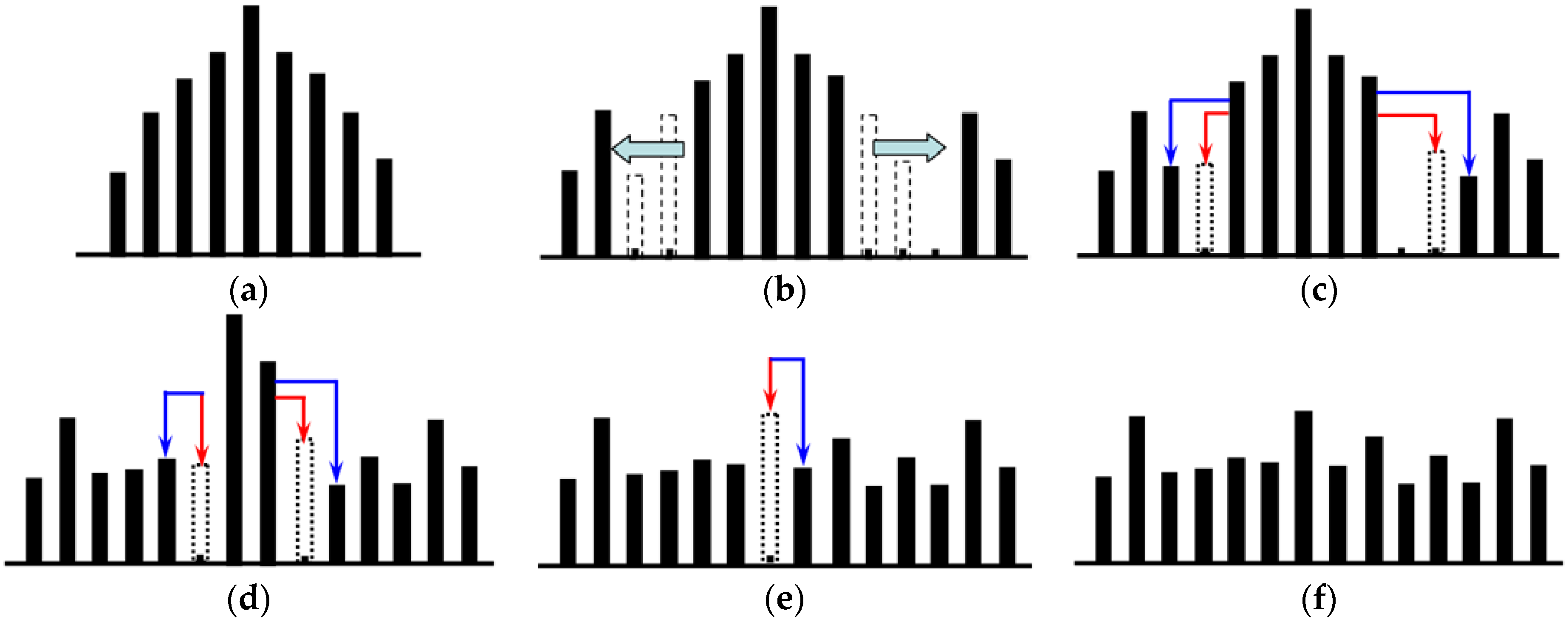
45] proposed a reversible watermarking scheme for images based on multilevel histogram modification, in which reversible watermark embedding is performed by using multiple pairs that each consist of a peak point and zero point, which significantly increases the embedding capacity. The main steps of the watermark embedding are as follows:
Step 1: The image is performed with the inverse “
S” order scan, and the difference histogram is constructed using adjacent pixels, as shown in
Figure 1a.
Step 2: The number of embedding levels is chosen based on the number of watermarks to be embedded. Without loss of generality, taking
L = 2 as an example, as shown in
Figure 1b, the bins that are greater than
L are shifted towards the right by
L + 1, whereas those that are less than -
L are shifted towards the left by
L, which generates a new difference histogram.
Step 3: The bins in the difference histogram that are equal to ±
L are modified, as shown in
Figure 1c, by combining the watermarks to be embedded, in which the bins in the dotted line indicated by red arrows are the bins that are embedded with the watermark bit of “0” after modification, and the bins in the solid line indicated by the blue arrows are the bins that are embedded with the watermark bit of “1” after modification (the same as below). After the modification is completed, the value of
L is decreased by 1.
Step 4: Repeat
Step 2–Step 3 until
L = 0, as shown in
Figure 1d.
Step 5: If
L = 0, then the bins with a difference histogram equal to 0 are modified, as shown in
Figure 1e, which gives rise to the final watermarked difference histogram, as shown in
Figure 1f.
Step 6: The watermarked pixel values are calculated based on the differences after modification, and the watermarked images are generated according to the scan sequence.
The processes of watermark extraction and carrier recovery are the inverse process of watermark embedding. The main steps are as follows:
Step 1: The image to be detected undergoes the inverse “S” order scan.
Step 2: The watermarked difference is calculated using the recovery value of the previous pixel and the current pixel value. According to the interval of the watermarked difference, the corresponding original difference is recovered in the inverse process of
Figure 1.
Step 3: Adopting the sequential recovery strategy, the current pixel value is recovered using the recovery value of the previous pixel and the corresponding original difference value.
Step 4: The watermark is extracted on the watermarked difference values obtained in Step 2 of the watermark extraction procedure according to the set rules, and the L value is decreased by 1. Repeat this step until L = 0.
Step 5: If
L = 0, the watermark is extracted in the inverse process of
Figure 1e.
Step 6: The watermark bit extracted at each level is sequentially connected, which gives rise to the watermarks hidden in the carrier.
In Zhao’s reversible watermarking scheme, the multilevel histogram modification effectively increases the embedding capacity, and the largest change in the pixel values of the original image carrier is L + 1, with good imperceptibility.
2.3. Analysis of Vector Map Histogram Features
Since there is a significant difference between the vector map difference histogram and raster image difference histogram, Zhao’s scheme cannot be directly applied to the vector map data. Extensive experimental analyses show that the distribution characteristics of the vector map difference histogram are as follows:
(1) Difference in sharpness
Vector maps of different element types, such as rivers, roads, residential areas, or landforms, differ in their histogram sharpness. In general, a sharp histogram has a large embedding capacity, whereas a flat histogram has a small embedding capacity.
(2) Uncertain position of the peak point
In a raster image, neighbouring pixels exhibit little difference, and the peak point of the difference histogram is usually at a position with a difference of zero. In a vector map, the position of the peak point of the difference histogram is uncertain, and the positions of the peak points of the map data of different types and scales vary.
(3) Poor continuity
The coordinates of adjacent points on the same entity and between different entities jump, which leads to many zero points in the difference histogram. From the perspective of the distribution shape, the continuity of the histogram distribution is not strong.
(4) Wide distribution
For a 256-level raster image, the distribution interval with the largest pixel difference is [−255, 255], but the difference range of the vector map is associated with the frame size, scale, and coordinate type, and for the sake of ease of computation, the floating-point coordinates must be converted to integer coordinates, which leads to a wide distribution in the difference histogram.
In summary, to meet the needs of practical applications, it is necessary to design a reversible watermarking algorithm that is truly applicable to vector maps by closely following the characteristics of the vector map data.
3. Proposed Reversible Watermarking Scheme
The proposed reversible watermarking scheme for the vector maps based on multilevel histogram modification is mainly composed of three parts: construction and processing of the histogram, watermark embedding, watermark extraction and data recovery. The detailed process for each part is described below.
3.1. Histogram Construction and Processing
A vector map consists of several entities, with each entity composed of a series of vertices, and the coordinates of each vertex include the x-axis coordinate and the y-axis coordinate. Therefore, the vertices of a vector map can be expressed as , in which and are, respectively, the horizontal and vertical coordinates of the ith vertex and N is the total number of coordinate points.
Due to the presence of measurement error in the vector map, the horizontal and vertical coordinates have precision bits, changes in which do not affect the normal use of the data. After reversible watermarks are extracted, the carrier data can be recovered losslessly; nevertheless, to not affect the normal use of the watermarked data and to avoid arousing the attacker’s suspicion, the modification of the carrier data should be minimal. In general, double-precision floating-point coordinates can represent up to 16–17 significant digits. To make it easier to construct a difference histogram, the floating point coordinates in the map
are decomposed into integer coordinates
and decimal coordinates
, as shown in Equation (1):
Here, is the rounding down function, and t is the selected number of digits after the decimal point; if we let the number of decimal digits of the coordinates be e and the precision bit be the pth decimal digit, then p < t < e. Below, the x-axis coordinate is used as an example to describe the proposed reversible watermarking scheme; that of the y-axis can be operated similarly and is thus omitted here.
Since the coordinates of adjacent points exhibit a certain correlation, to obtain a greater peak value of the histogram, the coordinate difference between adjacent points is calculated using Equation (2).
The difference histogram of the vector map is then constructed based on the statistics of the differences.
Let the embedding level of the reversible watermark be L, which is closely related to the watermark capacity and the quality of the vector map after the watermark embedding. The greater the value of L is, the greater the embedding capacity and the higher the embedded map data error, and vice versa. Based on its distribution characteristics, the vector map histogram is divided into continuous regions and discontinuous regions.
Definition 1. In a difference histogram, for a histogram bin with a difference of h, if its neighbouring region L (i.e., the region of) does not exhibit any zero point, then the region is called a continuous region, and if the region shows any zero points, the region is then called a discontinuous region; the histogram bin with a difference of h is called the central bin of this region.
Thus, there are the following properties: (1) continuous and discontinuous regions together constitute the entire difference histogram; (2) each continuous region has a total of 2L + 1 histogram bins; (3) the sum of the frequencies of all histogram bins within the neighbouring region L of the maximum peak point of the histogram is not necessarily the maximum; and (4) after histogram shifting, the properties of the continuous and discontinuous regions remain unchanged.
3.2. Watermark Embedding
The overall flowchart of the watermark embedding process is shown in
Figure 2. When embedding watermarks, we divide the constructed difference histogram into continuous regions and discontinuous regions and embedded watermarks in the two types of regions by adopting different histogram modification strategies, ultimately giving rise to watermarked vector map data.
The specific steps of the watermark embedding procedure are as follows:
Step 1: As described in
Section 3.1, the coordinates of all vertices of the vector map are extracted and converted to integer coordinates. The difference histogram is then constructed based on the integer coordinates of adjacent points, and the histogram is divided into continuous and discontinuous regions.
Step 2: Let the central bin of a continuous region be
h, and let
be the function that is used to calculate the frequency of the histogram bin; the sum of the frequencies of all histogram bins in this continuous region (
S) is calculated using Equation (3):
After traversing all of the continuous regions, the continuous region with the highest value is chosen, and the point that corresponds to the central bin in this region is the optimal peak point of the entire histogram, which is denoted as dp
Step 3: In each of the discontinuous regions on the left half portion of the optimal peak point (), the left peak point () is chosen based on the histogram bin with the highest frequency, and the zero point that is smaller than and closest to is chosen as the left zero point (). Similarly, in each of the discontinuous regions on the right half portion of the optimal peak point (), the right peak point () and right zero point () are chosen. Given the positional relationship, the intervals of and do not overlap with each other, i.e., .
Step 4: The histogram shifting is operated using Equation (4), in which the histogram bins to the right of
are shifted to the right by
L+1 and those to the left of
are shifted to the left by
L, whereas the remaining histogram bins are kept unchanged.
Step 5: According to the current embedding level of
L, the processed differences are modified using Equation (5):
Here, w is the watermark bit of the embedded watermark. After completing the modification on all of the differences, the L value is subtracted by 1.
Step 6: Repeat
Step 5 until
L = 0. When
L = 0, the 0th-level watermark is embedded using Equation (6):
Step 7: After the histogram shifting, the properties of the continuous and discontinuous regions remain unchanged; thus, the watermark embedding is continued in the discontinuous region of the histogram using Equation (7):
Step 8: The integer part of the watermarked
x-axis coordinate is calculated using Equation (8):
Step 9: The complete watermarked
x-axis coordinate is calculated using Equation (9):
At this point, the watermark embedding process on the x-axis coordinate is completed. The same operation is performed on the y-axis coordinate to obtain the final watermarked vector map data.
3.3. Watermark Extraction and Data Recovery
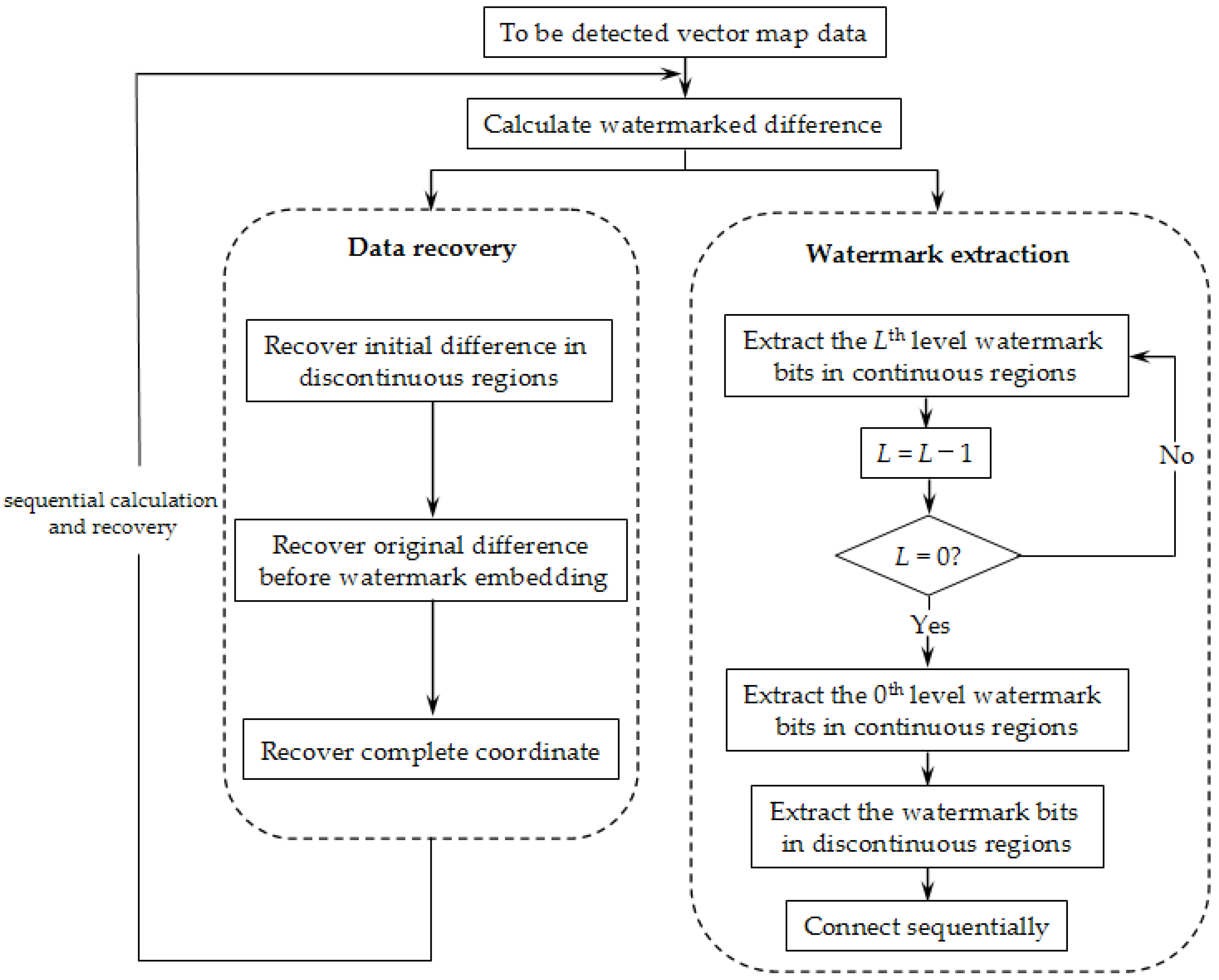
The overall flowchart of the watermark extraction and data recovery processes is shown in
Figure 3. The process of watermark extraction and data recovery is the reverse of the embedding process, and the overall idea of recovering the carrier data first and then extracting the watermark is adopted. When building the implementation, the strategy of sequential calculation and recovery is adopted.
The detailed steps of the watermark extraction procedure are as follows:
Step 1: As described in
Section 3.1, the coordinates of all vertices of the test vector map are extracted, and they are decomposed into integer coordinates and decimal coordinates using Equation (1). The differences with hidden watermarks are sequentially calculated using Equation (10):
Here, is a known value, and it remains unchanged during the watermark embedding, extracting, and data recovery processes, i.e., .
Step 2: The calculated difference values are performed with an initial recovery using Equation (11):
After this operation, the differences in the intervals of and are recovered to the values before watermark embedding.
Step 3: Next,
is recovered to the original difference using Equation (12):
Step 4: The integer part of the
x-axis coordinate is recovered using Equation (13):
Step 5: In combination with the decimal coordinate, the complete
x-axis coordinate is then recovered using Equation (14):
It should be noted that in recovering the carrier data, Steps 1–5 are iterated, and the map coordinates are recovered sequentially and individually.
Step 6: The watermarks embedded in the continuous regions are extracted level by level using Equation (15):
After completing the watermark extraction at each level, the L value is decreased by 1. In the equation, WL represents the watermark extracted at level L.
Step 7: Repeat Step 6 until
L = 0. When
L = 0, the watermark extraction at level 0 is performed using Equation (16):
Step 8: The watermarks hidden in discontinuous regions are extracted using Equation (17):
Step 9: The above-extracted watermarks are sequentially connected to form a final watermark (
w):
At this point, the process of watermark extraction and data recovery of the x-axis coordinates is completed.
4. Experimental Results and Analysis
To verify the performance of the proposed algorithm, the following series of experiments were performed on the VS2010 and MATLAB R2012b development platforms under the Windows 7 operating system. The hardware environment of the computer was as follows: an Intel(R) Core(TM) i5-2400 CPU (3.10 GHz) with 4 GB of RAM and an NVIDIA GeForce 605 graphics card. We performed simulation experiments using the data from 50 vector maps with different scales and different element types, and the performance of the algorithm was comprehensively evaluated in terms of the invisibility, reversibility, watermark capacity, and time complexity. The data used in this study are presented in
Figure 4; they are contour data, river data, road data, and habitation data. In
Table 1, the scale, entity number, vertex number, and error tolerance of the data of the four maps are presented.
4.1. Invisibility
Invisibility is an important indicator to evaluate the performance of a reversible watermarking algorithm. The embedded watermarks should have a minimal disturbance to the vector map. The root mean square error (RMSE) was used as the indicator for the data error, with the following equation:
Here, V and V′ are coordinate sets to be compared, and N is the total number of vertices. The lower the RMSE value is, the smaller the difference between V and V’; the greater the RMSE value is, the greater the difference between V and V’. If V and V’ are the original data and the watermarked data, then the lower the RMSE value is, the lower the error of the watermarked data.
In the proposed reversible watermarking algorithm, the error of the watermarked data depends on two main aspects: the number of the rounding decimal bit of the coordinate (
t) and the embedding level (
L). To verify the influence relationship between them, in the experiment shown in
Figure 5a, for
L = 2, the relationship between
t and RMSE was examined with varying
t values, and in the experiment shown in
Figure 5b, for
t = 5, the relationship between
L and RMSE was examined with varying
L values.
Figure 5 shows that for the same map data, when
L was constant, the higher the value of
t was, the lower the error of the carrier map data derived from the watermark embedding; when
t was constant, the higher the value of
L was, the higher the error of the carrier map data derived from the watermark embedding. Theoretically, the maximum change in the data caused by the histogram shifting in continuous regions is
, and the maximum change in the data caused by the histogram shifting in discontinuous regions is
; thus, after the multilevel histogram shifting, the maximum change on the data is
. Overall, the error of the watermarked coordinates caused by the proposed algorithm was behind the decimal digit of the precision requirement, so it did not affect the normal use of the map data, with good invisibility.
4.2. Analysis of Reversibility
It is required that after watermark extraction is completed, the carrier data are recovered losslessly, which is of great significance for vector maps with an extremely high precision requirement. Since computers cannot accurately store floating point data, as long as the RMSE between the recovered coordinates and the original coordinates is less than
, the recovery is regarded as reversible. The number of rounding decimal digits (
t) and the embedding level (
L) are designated as parameters (
t,
L); to verify the reversibility of the algorithm, different values of (
t,
L) were chosen randomly, and the lossless recovery was performed on the corresponding processed data. The RMSE values for the processed data and the original data was calculated, and the experimental results are reported in
Table 2.
Table 2 indicates that the RMSE values of the recovered data and the original data were all maintained below the order of 10
−17, which indicates that after the watermark extraction, the map data were recovered to their original state, and thus the algorithm was fully reversible and met the demand of vector maps for high precision.
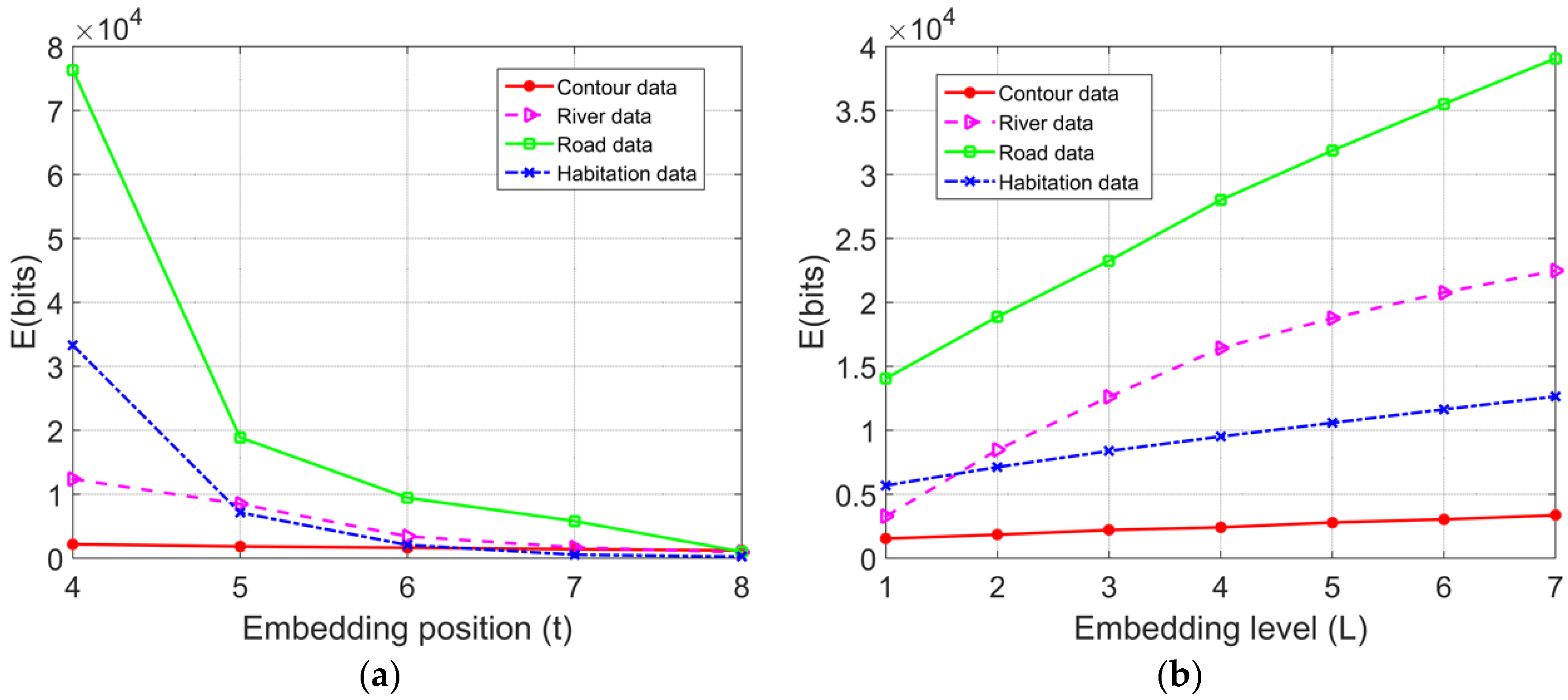
4.3. Watermark Capacity
The watermark capacity refers to the maximum number of watermarks that can be embedded in the vector map, which is an important criterion for evaluating the performance of a reversible watermarking algorithm. In general, the embedding capacity of the reversible watermark of the conventional histogram shifting is closely related to the magnitude of the peak value. In the proposed algorithm, the embedding capacity is the sum of the numbers of embedded watermarks in both the continuous and discontinuous regions; by using Equation (3), the watermarking capacity
E (bits) of the proposed reversible watermarking scheme is deduced:
It can be inferred that the embedding capacity of the proposed algorithm depends on the embedding level
L and the magnitude of each peak value; the latter is directly determined by the correlation of the adjacent data. Therefore, the watermark capacity is comprehensively affected by the number of rounding decimal digits (embedding position,
t) and the embedding level (
L). In the experiment shown in
Figure 6a, under
L = 2, the relationships between
t and
E were examined with varying values of
t; in the experiment shown in
Figure 6b, under
t = 5, the relationships between
L and
E were examined with varying values of
L.
The experimental results show that with the same map data, when L was constant, as t increases, the correlation between the adjacent data gradually weakened, which results in the decreased magnitude of the peak value of the difference histogram constructed through adjacent coordinates, and thus there is a reduced watermark embedding capacity; when t was constant, as L increased, the number of histogram bins that were involved in watermark embedding increased, and the overall watermark embedding capacity assumed an upward trend, while the increasing rate was associated with the features of the vector map data. In the process of watermark embedding, the embedding level L can be adaptively chosen according to the number of watermarks to be embedded.
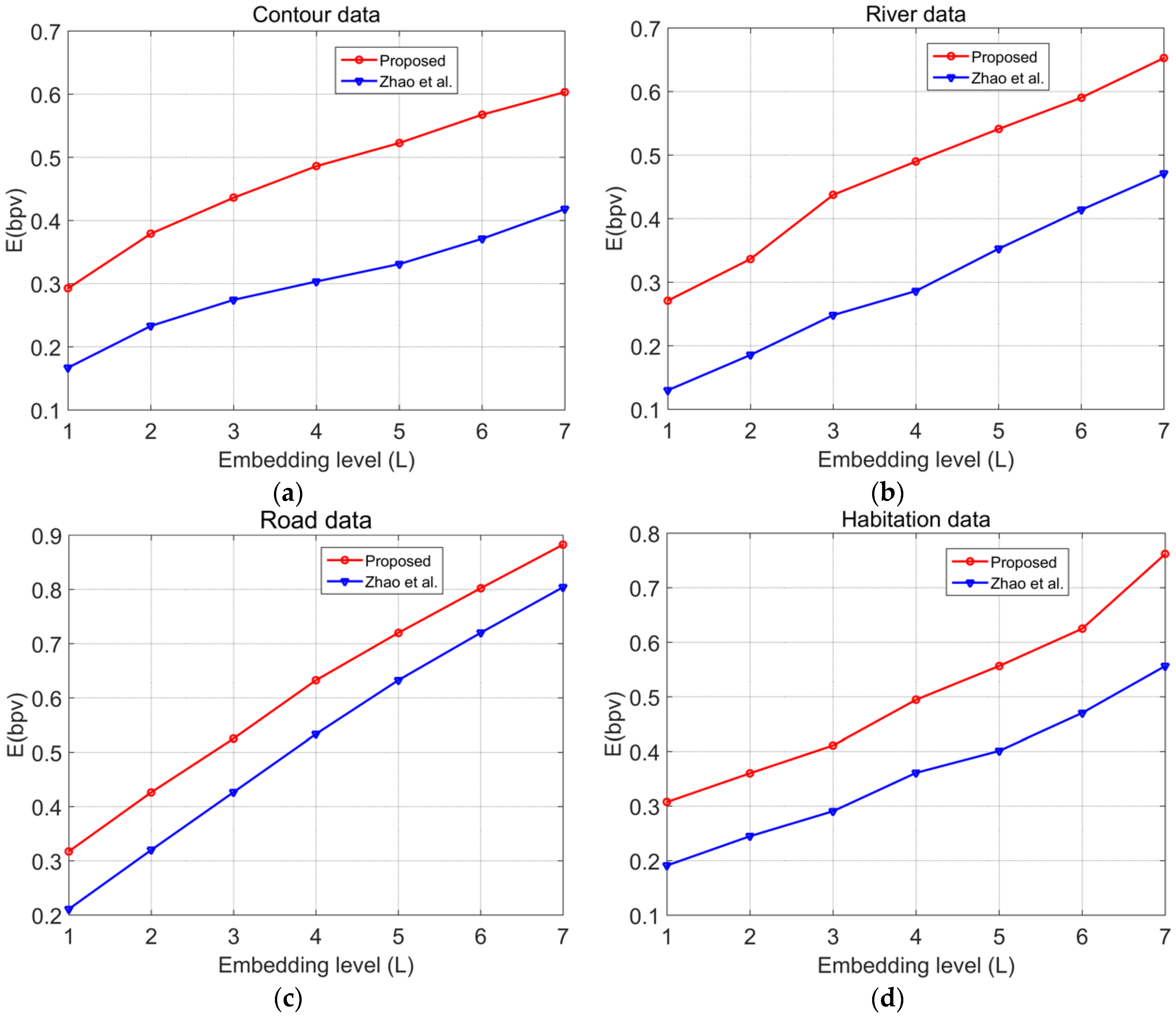
In the experiments shown in
Figure 7, Zhao’s algorithm [
45] was applied to the vector map data, and the resultant watermarking capacity was compared with the capacity obtained through the proposed algorithm. To increase the embedding capacity, the minimal value of
t was chosen under the premise that it did not affect the accuracy of the data under each scale. The bits per vertex (bpv) value was used to quantify the watermark capacity
E.
The experimental results show that in the data from four vector maps with different element types, the watermark capacities of the proposed algorithm were all higher than those of Zhao’s algorithm. This finding occurs because through multilevel histogram modification, the proposed algorithm achieved a higher watermark capacity. On one hand, the optimal peak value in continuous regions enabled us to maximise the capacity under the current embedding level. On the other hand, the involvement of the left and right maximal peak values in the discontinuous regions were fully utilised to embed the watermarks, whereas in Zhao’s method, only histogram bins in the region of are utilised to embed the watermarks; thus, the other bins are not fully utilised, and as a result, Zhao’s method is not suitable for vector map data.
To further verify the superiority of the proposed algorithm to similar algorithms, the proposed algorithm was compared with the algorithms presented in Refs. [
16,
26,
37]. The relationship between the watermark capacity
E (bpv) and the embedding distortion RMSE was used to evaluate the embedding performance of the algorithm; under the same watermark capacity, the lower the RMSE was, the higher the embedding performance of the algorithm, and similarly, under the same RMSE, the larger the watermark capacity was, the higher the embedding performance of the algorithm. In the experiments, the minimal value of
t was chosen under the premise that it did not affect the accuracy of the data under each scale; the experimental results are shown in
Figure 8.
The experimental results demonstrate that with the same embedding rate, the embedding distortion of the proposed algorithm was significantly less than that of other algorithms; with the same embedding distortion, the watermark embedding capacity of the proposed algorithm was significantly greater than that of other algorithms. Although the algorithm of Ref. [
26] achieved a high watermark embedding capacity, the multiple iterations of this method causes significant embedding distortion in the vector map data. The proposed algorithm effectively struck a balance between the embedding distortion and embedding capacity. In summary, compared with other algorithms, the proposed algorithm had a better embedding performance and was able to maintain a small embedding distortion even under a large embedding capacity.
4.4. Time Complexity
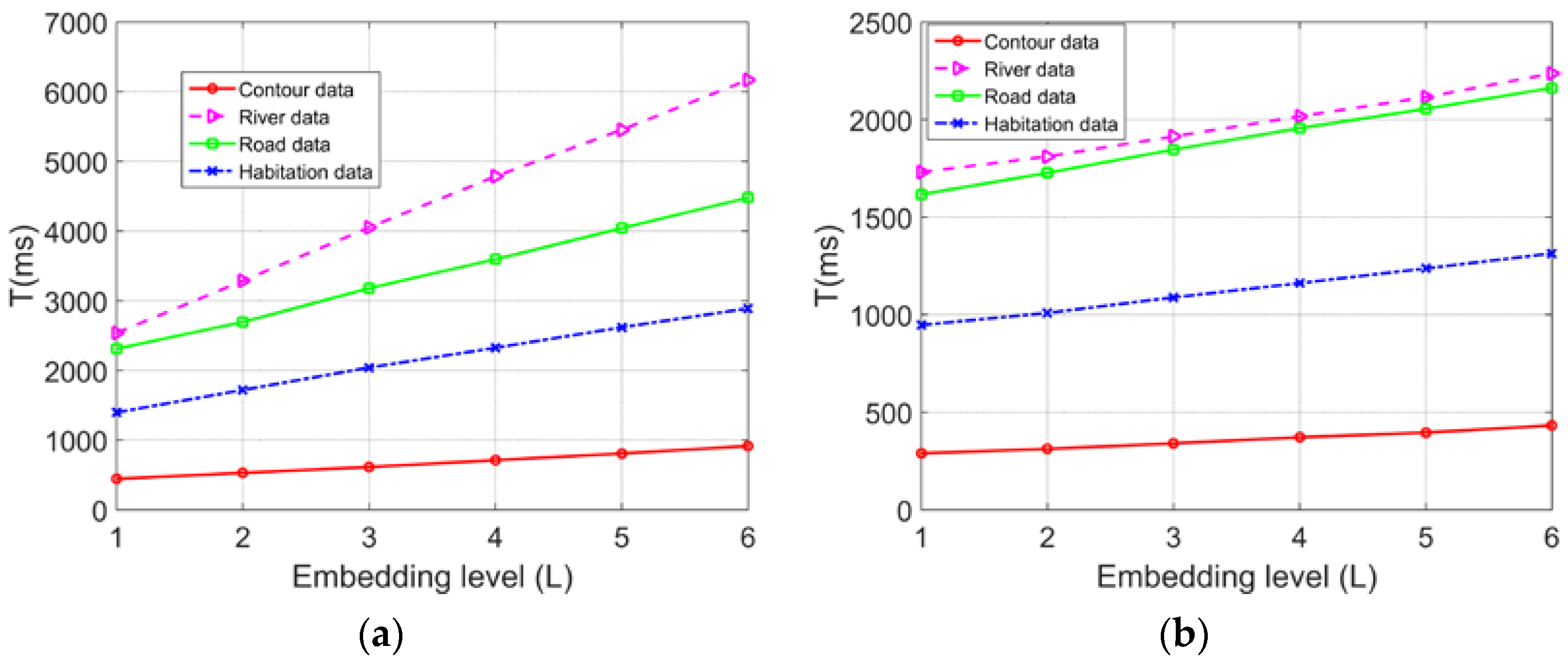
To evaluate the time complexity of the proposed algorithm, the times
T (ms) consumed for watermark embedding and detection at different embedding levels
L were compared using the four vector maps. The experimental results are shown in
Figure 9:
The experimental results showed that for the same vector map, the greater the value of the embedding level L was, the more time was consumed in executing the algorithm; for different vector maps, when the embedding level L was constant, the higher the total number of vertices was, and the longer it took for the algorithm to execute. In the watermark detection process, it was unnecessary to perform computations such as for the optimal peak value, so the watermark detection process required significantly less time than the watermark embedding process. Overall, the implementation of the proposed algorithm did not involve complex operations such as iteration, sorting, etc., and the times consumed in the processes of watermark embedding and extracting were essentially linear with low time complexity, thereby meeting the requirements of real-time embedding and detection in practical applications very well.
4.5. Application in Integrity Authentication
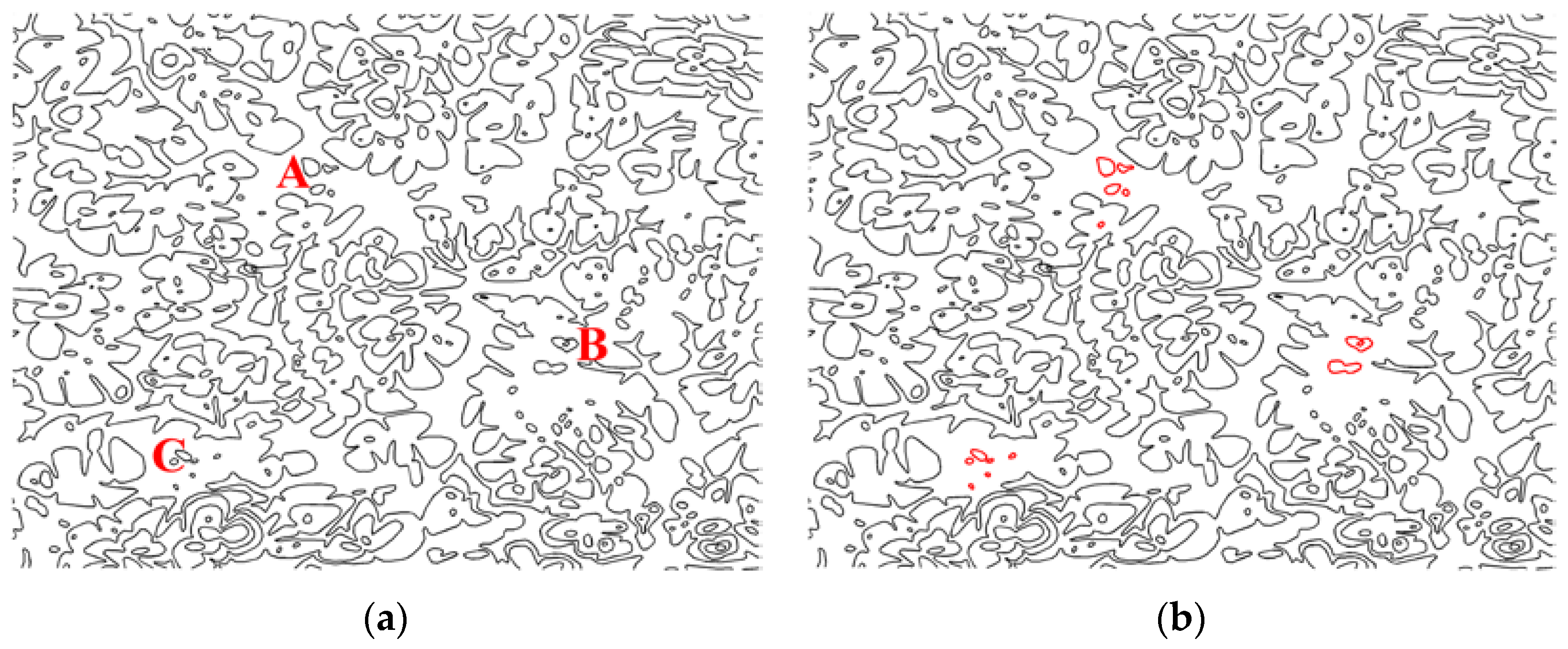
To evaluate the performance of the proposed algorithm in the integrity authentication of vector map data, the contour data in
Figure 4a was taken as an example for the experiment. First, entities in vector map were divided into groups, and all
x-axis coordinates and
y-axis coordinates in each group were used as inputs of the hash function to generate an authentication watermark. We then embedded the watermark into the original vector map data using the proposed method. Malicious tamper attacks were carried on the watermarked vector map, as shown in
Figure 10a, where an extra entity was added to Region A, an original entity was deleted from Region B, and an original entity was modified in Region C. The results of the tamper localization are shown in
Figure 10b.
The experimental results show that the proposed algorithm could be successfully applied to the integrity authentication of vector maps. After the watermarked vector map suffered from malicious tamper attacks on entities, such as addition, deletion, and modification, the proposed method could identify the tampered regions effectively, which exhibited an accurate tamper localization capability.


