New Concepts on Vertex and Edge Coloring of Simple Vague Graphs

Abstract

The vague graph has found its importance as a closer approximation to real life situations. A review of the literature in this area reveals that the edge coloring problem for vague graphs has not been studied until now. Therefore, in this paper, we analyse the concept of vertex and edge coloring on simple vague graphs. Specifically, two new definitions for vague graphs related to the concept of the λ-strong-adjacent and ζ-strong-incident of vague graphs are introduced. We consider the color classes to analyze the coloring on the vertices in vague graphs. The proposed method illustrates the concept of coloring on vague graphs, using the definition of color class, which depends only on the truth membership function. Applications of the proposal in solving practical problems related to traffic flow management and the selection of advertisement spots are mainly discussed.

1. Introduction

The concept of the fuzzy graph was proposed in the literature [1] with various definitions pertaining to the cycles, connectivity, and coloring of fuzzy graphs. Subsequently, the vertex strength and types of fuzzy graphs with operations were studied and investigated in the literature [2,3,4]. Some other works focused on the fuzzy total coloring and applications to a traffic light were introduced and studied by Lavanya and Sattanathan [5]; Jaiswal and Rai [6]; Samanta, Pramanik, and Pal [7]; and Kishore and Sunitha [8]. The density of fuzzy graphs, operations, and dual were introduced in the literature [9,10,11,12]. Ghorai and Pal [13] investigated the isomorphic properties of fuzzy graphs, whereas Ghorai and Pal [14] proposed the concept of regular bipolar fuzzy graphs and studied its applications. Fuzzy graph theory has also been extended to other extensions of fuzzy sets, such as vague sets.

In this paper, we study some new concepts related to the edge coloring of vague graphs. The vague set model was firstly introduced by Gau and Buehrer [15] in 1993, by replacing the membership degree of an element in a set with a subinterval between 0 and 1. A vague set, $A$, is described by a true membership function, $t_A(u_i)$, and a false membership function, $f_A(u_i)$, from the universe of discourse, $U$. Thus, the grade of membership of an element, $u_i$, in vague set, $A$, is bounded to the subinterval, $[t_A(u_i),1-f_A(u_i)]$ of $[0,1]$, and the sum of two degrees, that is, $t_A(u_i)$ and $f_A(u_i),$ must be less than 1.

In fuzzy set theory, the grade of membership of an object to a fuzzy set indicates the belongingness degree of the object to the fuzzy set, which is a point (single) value selected from the unit interval $[0,1]$. In real life scenarios, a person may consider that an element belongs to a fuzzy set, but it is possible that that person is not sure about it. Therefore, hesitation or uncertainty may exist in which the element can belong to the fuzzy set or not. The traditional fuzzy set is unable to capture this type of hesitation or uncertainty using only the single membership degrees. A possible solution is to use an intuitionistic fuzzy set or a vague set [15] to handle this problem. For example, in a traffic control system of a city, 10 sensors $\left\{s_1,s_2,s_3,\dots ,s_{10}\right\}$ can be used to store the waiting time of traffic flow with 10 corresponding measurements $\left\{3,4,3,3,\_,3,5,\_,3,3\right\}$ at a specific time, t. Here, ‘_’ represents that the information of a sensor is not captured at time, t. We find three for six times, four for one time, five for one time, and two missing values. This uncertain information can be represented as a vague set, A, as follows. In the measurement, three occur for six times, but two values (i.e., 4 and 5) are against it and two values are missing values. The true membership degree $t_A(u_i)$ and false membership degree $f_A(u_i)$ are 0.6 and 0.2$\left(1-f_A(u_i)=0.8\right)$, respectively. The vague membership degree is computed as $\left[0.6,0.8\right]$ for three. Similarly, the vague membership degree is obtained $\left[0.1,0.3\right]$ for four, and $\left[0.1,0.3\right]$ for five. The vague set can be represented as $A=\raisebox{1ex}{$\left[0.6,0.8\right]$}\!\left/ \!\raisebox{-1ex}{$3$}\right.+\raisebox{1ex}{$\left[0.1,0.3\right]$}\!\left/ \!\raisebox{-1ex}{$4$}\right.+\raisebox{1ex}{$\left[0.1,0.3\right]$}\!\left/ \!\raisebox{-1ex}{$5$}\right.$. The above real-life problem describes that, by using a vague set, it is more capable to manage the uncertain information than fuzzy set [16].

Some concepts related to vague graphs, such as the Laplacian matrix and spectrum, were introduced in Borzooei and Rashmanlou [17], whereas the isomorphic properties of vague graphs were studied in Talebi et al. [18]. Borzooei, Rashmanlou, and Mathew [19] defined the homomorphism of vague graphs. Samanta et al. [20] studied the behaviour of vague graphs, and presented an investigation on the strength of vague graphs, which was then further investigated in [21]. Rashmanlou et al. [22] introduced vague h-morphism. Darabian et al. [23] studied the concepts of regularity and irregularity in the study of fullerene molecules, wireless multihop networks, and road transport networks. Borzooei and Rashmanlou [24] introduced further results on vague graphs in the form of three types of new product operations of vague graphs and verified the rationality of these concepts. Borzooei et al. [25] introduced the concept of strong domination numbers of vague graphs and presented methods to determine the strong domination numbers for any complete vague graph.

The edge coloring problem is an important area of study in fuzzy graph theory, which could be used to solve many real life problems (such as traffic, etc.) [4,5,6,7,8]. The main contribution of this paper is as follows.

• In the literature, to the best of our knowledge, there is no study on the edge coloring problem for vague graphs until now. Therefore, in this paper we study the concept of vertex and edge coloring on simple vague graphs.
• We also demonstrate the utility of these concepts in solving practical problems related to traffic flow management and selection of advertisement spots that will optimize the visibility of the advertisements.
• We also introduce the idea of $\lambda$-strong-adjacent and $\zeta$-strong-incident of vague graphs.

2. Preliminary

For the remaining part of this paper, the collection of all fuzzy sets on a set, $S$, shall be denoted by $\mathfrak{F}\left(S\right)$. The symbol $\wedge$ shall be used to denote a T-norm function (e.g., the minimum), with $\vee$ being its respective T-conorm (i.e., S-norm).

Definition 1

[5].Let$V$be a set. Let$\sigma :V\to \left[0,1\right]$and$\mu :V\times V\to \left[0,1\right]$be two functions satisfying$\mu \left(x,y\right)\le \sigma \left(x\right)\wedge \sigma \left(y\right)$for all$x,y\in V$. We have, the following:

(a) 

$\mathcal{G}=⟨V,\sigma ,\mu ⟩$ is said to be a fuzzy graph;

(b) 

$V$is said to be the vertex set of$\mathcal{G}$. Each$x\in V$is said to be a vertex in$\mathcal{G}$;

(c) 

$V\times V$is said to be the edge set of$\mathcal{G}$. Each$\left(x,y\right)\in V\times V$is said to be an edge * in$\mathcal{G}$;

(d) 

$\sigma \left(x\right)$is said to be the membership value of the vertex$x$in$\mathcal{G}$;

(e) 

$\mu \left(x,y\right)$is said to be the membership value of the edge *$\left(x,y\right)$in$\mathcal{G}$.

Remark 1. 

In the literature [5], it was assumed that$\mu \left(x,y\right)=\mu \left(y,x\right)$and$\mu \left(x,x\right)=0$for all$x,y\in V$.

Definition 2

[5].Let$\mathcal{G}=⟨V,\sigma ,\mu ⟩$be a fuzzy graph. Let$u,v$be two vertices in$\mathcal{G}$. If$\mu \left(u,v\right)\ge \frac{1}{2}\left(\sigma \left(u\right)\wedge \sigma \left(v\right)\right)$, then$u$and$v$are said to be strong adjacent to each other.

Definition 3

[5].Let$\mathcal{G}=⟨V,\sigma ,\mu ⟩$be a fuzzy graph. Let$k\in \mathbb{N}$. Let$C=\left\{{\gamma }_i\in \mathfrak{F}\left(V\right):1\le i\le k\right\}$for which

(i)${{\displaystyle \mathrm{U}}}_{1\le i\le k}{\gamma }_i=\left\{\left(x,\sigma \left(x\right)\right),x\in V\right\}$;

(i.e.,${\displaystyle {\mathrm{V}}_{1\le i\le k}}({\gamma }_i\left(x\right))=\sigma \left(x\right)$for all$x\in V$);

(ii)${\gamma }_i\cap {\gamma }_j=\varnothing$;

(i.e.,${\gamma }_i\left(x\right)\wedge {\gamma }_j\left(x\right)=0$for all$x\in V$), for all$i\ne j$;

(iii) for each pair of strongly adjacent$u,v\in V$, we have he following:

$${\gamma }_i\left(u\right)\wedge {\gamma }_i\left(v\right)=0 for alli.$$

Then,$ℭ$is said to be a$k$-fuzzy vertex coloring of$\mathcal{G}$.

Definition 4

[5].Let$\mathcal{G}=⟨V,\sigma ,\mu ⟩$be a fuzzy graph. The least value of$k\in \mathbb{N}$, for which a$k$-fuzzy vertex coloring of$\mathcal{G}$exist, is called the fuzzy vertex chromatic number of$\mathcal{G}$, and shall be denoted by${\mathcal{X}}_{\mathfrak{F}}\left(\mathcal{G}\right)$.

Definition 5

[5].Let$\mathcal{G}=⟨V,\sigma ,\mu ⟩$be a fuzzy graph. Let$h\in \mathbb{N}$. Let$D=\left\{{\phi }_i\in \mathfrak{F}\left(V\times V\right):1\le i\le h\right\}$for which

(i)${{\displaystyle \mathrm{U}}}_{1\le i\le h}{\phi }_i=\left\{\left(\left(x,y\right),\mu \left(x,y\right)\right),\left(x,y\right)\in V\times V\right\}$.

(i.e.,${\mathrm{V}}_{1\le i\le h}({\phi }_i\left(x,y\right))=\mu \left(x,y\right)$for all$\left(x,y\right)\in V\times V$)

(ii)${\phi }_i\cap {\phi }_j=\varnothing$(i.e.,${\phi }_i\left(x,y\right)\wedge {\phi }_j\left(x,y\right)=0$for all$\left(x,y\right)\in V\times V$), for all$i\ne j$.

(iii) for each$u\in V$, and for each$\left(v,u\right)$and$\left(w,u\right)$strong incident towards$u$:

$${\phi }_i\left(v,u\right)\wedge {\phi }_j\left(w,u\right)=0 for alli.$$

Then,$\mathfrak{D}$is said to be a$h$-fuzzy edge coloringof$\mathcal{G}$.

Definition 6

[5].Let$\mathcal{G}=⟨V,\sigma ,\mu ⟩$be a fuzzy graph. The least value of$h\in \mathbb{N}$, for which a$k$-fuzzy edge coloring of$\mathcal{G}$exists, is called the fuzzy edge chromatic number of$\mathcal{G}$, and shall be denoted by${\mathcal{E}}_{\mathfrak{F}}\left(\mathcal{G}\right)$.

Definition 7

[26].Let$V$be a set. Let$A=\left\{\left(x,\left[t_A\left(x\right),1-f_A\left(x\right)\right]\right),x\in V\right\}$, where$t_A,f_A:V\to \left[0,1\right]$are two functions satisfying$t_A\left(x\right)+f_A\left(x\right)\le 1$for all$x\in V$. Then, we have the following:

(a) 

$A$is said to be a vague set on$V$;

(b) 

$t_A\left(x\right)$is said to be the least membership of$x$in$V$;

(c) 

$1-f_A\left(x\right)$is said to be the greatest membership of$x$in$V$.

Remark 2. 

$\left[t_A\left(x\right),1-f_A\left(x\right)]\subseteq [0,1\right]$for all$x$.

For the remaining part of this paper, the collection of all vague sets on a set$S$shall be denoted by$\mathfrak{U}\left(S\right)$.

Definition 8

[17].Let$V$be a set. Let$\breve{\sigma }=\left(t_{\breve{\sigma }},f_{\breve{\sigma }}\right)$and$\breve{\mu }=\left(t_{\breve{\mu }},f_{\breve{\mu }}\right)$, where$t_{\breve{\sigma }},f_{\breve{\sigma }}:V\to \left[0,1\right]$and$t_{\breve{\mu }},f_{\breve{\mu }}:V\times V\to \left[0,1\right]$are four functions satisfying the following:

(i)$t_{\breve{\sigma }}\left(x\right)+f_{\breve{\sigma }}\left(x\right)\le 1$and$t_{\breve{\mu }}\left(x,y\right)+f_{\breve{\mu }}\left(x,y\right)\le 1$for all$x,y\in V$;

(ii)$t_{\breve{\mu }}\left(x,y\right)\le t_{\breve{\sigma }}\left(x\right)\wedge t_{\breve{\sigma }}\left(y\right)$and$f_{\breve{\mu }}\left(x,y\right)\ge f_{\breve{\sigma }}\left(x\right)\vee f_{\breve{\sigma }}\left(y\right)$for all$x,y\in V$.

Then, we have the following:

(a) 

$\mathcal{G}=⟨V,\breve{\sigma },\breve{\mu }⟩$is said to be a vague graph;

(b) 

$V$is said to be the vertex set of$\mathcal{G}$. Each$x\in V$is said to be a vertex in$\mathcal{G}$;

(c) 

$V\times V$is said to be the edge set of$\mathcal{G}$. Each$\left(x,y\right)\in V\times V$is said to be a directed edge in$\mathcal{G}$;

(d) 

$t_{\breve{\sigma }}\left(x\right)$is said to be the least membership value of the vertex$x$in$\mathcal{G}$;

(e) 

$1-f_{\breve{\sigma }}\left(x\right)$is said to be the greatest membership value of the vertex$x$in$\mathcal{G}$;

(f) 

$t_{\breve{\mu }}\left(x,y\right)$is said to be the least membership value of the directed edge$\left(x,y\right)$in$\mathcal{G}$;

(g) 

$1-f_{\breve{\mu }}\left(x,y\right)$is said to be the greatest membership value of the directed edge$\left(x,y\right)$in$\mathcal{G}$.

Definition 9

[17].Let$\mathcal{G}=⟨V,\breve{\sigma },\breve{\mu }⟩$be a vague graph. Let$u,v$be two distinct vertices in$\mathcal{G}$. If both$t_{\breve{\mu }}\left(v,u\right)=t_{\breve{\mu }}\left(u,v\right)$and$f_{\breve{\mu }}\left(v,u\right)=f_{\breve{\mu }}\left(u,v\right)$holds, then$\left\{u,v\right\}=\left\{\left(v,u\right),\left(u,v\right)\right\}$is said to be an (ordinary) edge in$\mathcal{G}$.

Definition 10

[17].Let$\mathcal{G}=⟨V,\breve{\sigma },\breve{\mu }⟩$be a vague graph. If both$t_{\breve{\mu }}\left(y,x\right)=t_{\breve{\mu }}\left(x,y\right)$and$f_{\breve{\mu }}\left(y,x\right)=f_{\breve{\mu }}\left(x,y\right)$holds for all$x,y\in V$, then$\mathcal{G}$is said to be ordinary. Otherwise,$\mathcal{G}$is said to be directed.

Definition 11

[17].Let$\mathcal{G}=⟨V,\breve{\sigma },\breve{\mu }⟩$be a vague graph. If both$t_{\breve{\mu }}\left(x,x\right)=0$and$f_{\breve{\mu }}\left(x,x\right)=1$holds for all$x\in V$, then$\mathcal{G}$ is said to be simple.

To facilitate further discussion, we present two new definitions (Definitions 12 and 13) for vague graphs, related to the concept of$\lambda$-strong-adjacent and$\zeta$-strong-incident of vague graphs.

Definition 12

Let$\mathcal{G}=⟨V,\breve{\sigma },\breve{\mu }⟩$be a vague graph. Let$u,v$be two vertices in$\mathcal{G}$. Let$\lambda \in \left[0,1\right]$. If both

$$t_{\breve{\mu }}\left(u,v\right)\ge \lambda \left(t_{\breve{\sigma }}\left(u\right)\wedge t_{\breve{\sigma }}\left(v\right)\right) and{f}_{\breve{\mu }}\left(u,v\right)\le \left(1-\lambda \right)+\lambda \left(f_{\breve{\sigma }}\left(u\right)\vee f_{\breve{\sigma }}\left(v\right)\right)$$

holds, then$u$is said to be$\lambda$-strong adjacent to$v$. Moreover, if both$t_{\breve{\mu }}\left(u,v\right)\wedge t_{\breve{\mu }}\left(v,u\right)\ge \lambda \left(t_{\breve{\sigma }}\left(u\right)\wedge t_{\breve{\sigma }}\left(v\right)\right)$and$f_{\breve{\mu }}\left(u,v\right)\vee f_{\breve{\mu }}\left(v,u\right)\le \left(1-\lambda \right)+\lambda \left(f_{\breve{\sigma }}\left(u\right)\vee f_{\breve{\sigma }}\left(v\right)\right)$holds, then$u$and$v$are said to be mutually$\lambda$-strong adjacent.

Remark 3. 

With regards to the definition, if$\lambda =\frac{1}{2}$(i.e., 50%), for instance, then$u$is said to be$\frac{1}{2}$strong adjacent (or 50% strong adjacent) to$v$.

Definition 13.

Let$\mathcal{G}=⟨V,\breve{\sigma },\breve{\mu }⟩$be a vague graph. Let$u,v$be two vertices in$\mathcal{G}$. Let$\zeta \in \left[0,1\right]$. If both

$$t_{\breve{\mu }}\left(u,v\right)\ge \zeta \left(t_{\breve{\sigma }}\left(v\right)\right) and f_{\breve{\mu }}\left(u,v\right)\le \left(1-\zeta \right)+\zeta \left(f_{\breve{\sigma }}\left(v\right)\right)$$

holds, then$\left(u,v\right)$is said to be$\zeta$-strong incident towards$v$.

Remark 4. 

With this definition, whenever$\left(u,v\right)$is$\zeta$-strong incident towards$v$,$u$is also$\zeta$-strong adjacent to$v$, because of$t_{\breve{\sigma }}\left(v\right)\ge t_{\breve{\sigma }}\left(u\right)\wedge t_{\breve{\sigma }}\left(v\right)$and$f_{\breve{\sigma }}\left(v\right)\le f_{\breve{\sigma }}\left(u\right)\vee f_{\breve{\sigma }}\left(v\right)$. The need for these definitions will be illustrated in the examples in the subsequent sections.

Definition 14

[22].Let$\mathcal{G}=⟨V,\breve{\sigma },\breve{\mu }⟩$be a vague graph.$\mathcal{G}$is said to be complete if$t_{\breve{\mu }}\left(x,y\right)=t_{\breve{\sigma }}\left(x\right)\wedge t_{\breve{\sigma }}\left(y\right)$and$f_{\breve{\mu }}\left(x,y\right)=f_{\breve{\sigma }}\left(x\right)\vee f_{\breve{\sigma }}\left(y\right)$for all$x,y\in V$.

Remark 5. 

When$\mathcal{G}$is complete, it is ordinary and with all pairs of vertices mutually 100% strong adjacent to each other.

Definition 15

[22].A vague graph is said to be Eulerian if all of the edges in the graph are strongly connected and have a cycle from any vertex as the origin and terminal.

3. Vertex and Edge Coloring on Simple Vague Graphs

In the previous section, we discussed the concept of level sets for identifying the vertex coloring on vague graphs. In this section, we consider the color classes to analyze coloring on vertices in vague graphs. The concept of coloring on vague graphs using the definition of color class depends only on the truth membership function, which is the lower bound of the vague set. We do not consider the lower bound of the vague set, which carries the negation of false membership values. The following definitions are only for the case of the truth membership values of the vague graphs.

Definition 16.

Let$\mathcal{G}=⟨V,\breve{\sigma },\breve{\mu }⟩$be a vague graph. Let$k\in \mathbb{N}$. Let$C_{\lambda ,k}=\left\{{{\rm Y}}_i\in \mathfrak{U}\left(V\right):1\le i\le k\right\}$for which

(i)${{\displaystyle \mathrm{U}}}_{1\le i\le k}{{\rm Y}}_i=\left\{\left(x,\left[t_{\breve{\sigma }}\left(x\right),1-f_{\breve{\sigma }}\left(x\right)\right]\right),x\in V\right\}$;

(i.e.,${\mathrm{V}}_{1\le i\le k}(t_{{\rm Y}}{}_i\left(x\right))=t_{\breve{\sigma }}\left(x\right)$and${\wedge }_{1\le i\le k}(f_{{\rm Y}}{}_i\left(x\right))=f_{\breve{\sigma }}\left(x\right)$for all$x\in V$)

(ii)${{\rm Y}}_i\cap {{\rm Y}}_j=\varnothing$

(i.e.,$t_{{\rm Y}}{}_i\left(x\right)\wedge t_{{\rm Y}}{}_j\left(x\right)=0$and$f_{{\rm Y}}{}_i\left(x\right)\vee f_{{\rm Y}}{}_j\left(x\right)=1$for all$x\in V$), for all$i\ne j$;

(iii) for each pair of mutually$\lambda$-strong adjacent$u,v\in V$, we have the following:

$$t_{{\rm Y}}{}_i\left(u\right)\wedge t_{{\rm Y}}{}_i\left(v\right)=0 and f_{{\rm Y}}{}_i\left(u\right)\vee f_{{\rm Y}}{}_i\left(v\right)=1 for alli.$$

Then,$C_{\lambda ,k}$is said to be a$\lambda$-strong$k$vague vertex coloring scheme (abbr.${\left[\lambda ,k\right]}_{\mathfrak{U}}$-VCS) of$\mathcal{G}$.

Definition 17.

Let$\mathcal{G}=⟨V,\breve{\sigma },\breve{\mu }⟩$be a vague graph. The least value of$k\in \mathbb{N}$, for which a$\lambda$-strong k-vague vertex coloring of$\mathcal{G}$exist, is called the$\lambda$-strong vague vertex chromatic number of$\mathcal{G}$, and shall be denoted by${\mathcal{X}}_{\mathfrak{U}}^{\left[\lambda \right]}\left(\mathcal{G}\right)$. Moreover, a$C_{\lambda ,k_0}$where$k_0={\mathcal{X}}_{\mathfrak{U}}^{\left[\lambda \right]}\left(\mathcal{G}\right)$is said to be a$\lambda$-strong minimal-vague vertex coloring scheme (abbr.${\left[\lambda ,min\right]}_{\mathfrak{U}}$-VCS) of$\mathcal{G}$.

Definition 18.

Let$\mathcal{G}=⟨V,\breve{\sigma },\breve{\mu }⟩$be a vague graph. Let$C_{\lambda ,k}=\left\{{{\rm Y}}_i\in \mathfrak{U}\left(V\right):1\le i\le k\right\}$be a${\left[\lambda ,k\right]}_{\mathfrak{U}}$-VCS of$\mathcal{G}$. Then,

(a) 

${𝓋}_i\left(C_{\lambda ,k}\right)={{\displaystyle \sum }}_{x\in V}\left(t_{{\rm Y}}{}_i\left(x\right)\right)$is said to be the minimum amount of${{\rm Y}}_i$by$C_{\lambda ,k}$on$\mathcal{G}$;

(b) 

$\mathcal{V}\left(C_{\lambda ,k}\right)={\mathrm{V}}_{1\le i\le k}{𝓋}_i\left(C_{\lambda ,k}\right)$is said to be the lower chromatic weight of$C_{\lambda ,k}$;

(c) 

${𝓌}_i\left(C_{\lambda ,k}\right)={{\displaystyle \sum }}_{x\in V}\left(1-f_{{\rm Y}}{}_i\left(x\right)\right)$is said to be the maximum amount of${{\rm Y}}_i$by$C_{\lambda ,k}$on$\mathcal{G}$;

(d) 

$\mathcal{W}\left(C_{\lambda ,k}\right)={\mathrm{V}}_{1\le i\le k}{𝓌}_i\left(C_{\lambda ,k}\right)$is said to be the upper chromatic weight of$C_{\lambda ,k}$.

Definition 19.

Let$\mathcal{G}=⟨V,\breve{\sigma },\breve{\mu }⟩$be a vague graph. Let$h\in \mathbb{N}$. Let$D_{\zeta ,h}=\left\{{\Phi }_i\in \mathfrak{U}\left(V\times V\right):1\le i\le h\right\}$for which

(i)${{\displaystyle \mathrm{U}}}_{1\le i\le h}{\Phi }_i=\left\{\left(\left(x,y\right),\left[t_{\breve{\mu }}\left(x,y\right),1-f_{\breve{\mu }}\left(x,y\right)\right]\right),\left(x,y\right)\in V\times V\right\}$;

(i.e.,${\mathrm{V}}_{1\le i\le h}(t_{\Phi }{}_i\left(x,y\right))=t_{\breve{\mu }}\left(x,y\right) and {\wedge }_{1\le i\le h}(f_{\Phi }{}_i\left(x,y\right))=f_{\breve{\mu }}\left(x,y\right)$)

for all$\left(x,y\right)\in V\times V$)

(ii)${\Phi }_i\cap {\Phi }_j=\varnothing$

(i.e.,$t_{\Phi }{}_i\left(x,y\right)\wedge t_{\Phi }{}_j\left(x,y\right)=0$and$f_{\Phi }{}_i\left(x,y\right)\vee f_{\Phi }{}_j\left(x,y\right)=1$for all$\left(x,y\right)\in V\times V$),

for all$i\ne j$;

(iii) for each$u\in V$, and for each$\left(v,u\right)$and$\left(w,u\right)$, both$\zeta$-strong incident towards$u$ are as follows:

$$t_{\Phi }{}_i\left(v,u\right)\wedge t_{\Phi }{}_i\left(w,u\right)=0 and f_{\Phi }{}_i\left(v,u\right)\vee f_{\Phi }{}_i\left(w,u\right)=1 for all i;$$

(iv) for each$u,v\in V$:$t_{\Phi }{}_i\left(v,u\right)=t_{\Phi }{}_i\left(u,v\right)$and$f_{\Phi }{}_i\left(v,u\right)=f_{\Phi }{}_i\left(u,v\right)$for all$i$.

Then,$D_{\zeta ,h}$is said to be a$\zeta$-strong$h$-vague edge coloring scheme (abbr.${\left[\zeta ,h\right]}_{\mathfrak{U}}$-ECS) of$\mathcal{G}$.

Definition 20.

Let$\mathcal{G}=⟨V,\breve{\sigma },\breve{\mu }⟩$be a vague graph. The least value of$h\in \mathbb{N}$, for which a$\zeta$-strong$h$-vague edge coloring of$\mathcal{G}$exist, is called the$\zeta$-strong vague edge chromatic number of$\mathcal{G}$, and shall be denoted by${\mathcal{E}}_{\mathfrak{U}}^{\left[\zeta \right]}\left(\mathcal{G}\right)$. Moreover, a$D_{\zeta ,h_0}$where$h_0={\mathcal{E}}_{\mathfrak{U}}^{\left[\zeta \right]}\left(\mathcal{G}\right)$is said to be a$\zeta$-strong minimal-vague edge coloring scheme (abbr.${\left[\zeta ,min\right]}_{\mathfrak{U}}$-ECS) of$\mathcal{G}$.

Definition 21.

Let$\mathcal{G}=⟨V,\breve{\sigma },\breve{\mu }⟩$be a vague graph. Let$D_{\zeta ,h}=\left\{{\Phi }_i\in \mathfrak{U}\left(V\times V\right):1\le i\le h\right\}$be a${\left[\zeta ,h\right]}_{\mathfrak{U}}$-ECS of$\mathcal{G}$. Then, we have the following:

(a) 

${𝓋}_i\left(D_{\zeta ,h}\right)={{\displaystyle \sum }}_{\left(x,y\right)\in V\times V}\left(t_{\Phi }{}_i\left(x,y\right)\right)$is said to be the minimum amount of${\Phi }_i$by$D_{\zeta ,h}$on$\mathcal{G}$;

(b) 

$\mathcal{V}\left(D_{\zeta ,h}\right)={\mathrm{V}}_{1\le i\le h}{𝓋}_i\left(D_{\zeta ,h}\right)$is said to be the lower chromatic weight of$D_{\zeta ,h}$;

(c) 

${𝓌}_i\left(D_{\zeta ,h}\right)={{\displaystyle \sum }}_{\left(x,y\right)\in V\times V}\left(1-f_{\Phi }{}_i\left(x,y\right)\right)$is said to be the maximum amount of${\Phi }_{i }$by$D_{\zeta ,h}$on$\mathcal{G}$;

(d) 

$\mathcal{W}\left(D_{\zeta ,h}\right)={\mathrm{V}}_{1\le i\le h}{𝓌}_i\left(D_{\zeta ,h}\right)$is said to be the upper chromatic weight of$D_{\zeta ,h}$.

4. Applications

4.1. Formation

Now, the formation of a vague graph in an example related to traffic flow and management in a fictitious town is given.

4.1.1. The Scenario

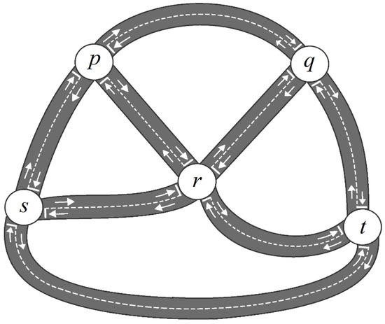
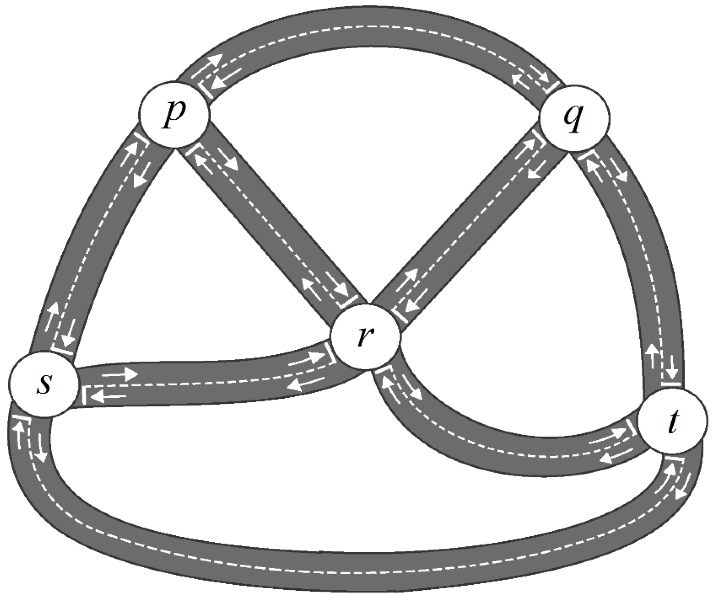
A region consists of five towns (not junctions), $p,q,r,s,t$, where most of the people live and/or work in. The towns are connected by roads, as shown in Figure 1.

Figure 1. The road map.

In particular, $r$ is the capital of the region, and there are many companies in $r$ providing delivery and GrabCar services to the other four towns.

The amount of traffic entering or leaving the region is deemed not significant, because most of the population who live in the region also work somewhere within it (can be in the same town or otherwise), and there is nothing in the region thatattracts tourists elsewhere. As a result, the total traffic amount in the region is assumed to be constant forall days of a year.

The amount of traffic on both sides of a given road are quite close. This is because if a person leaves his/her house to go to work or go shopping on a day, he/she will most likely return to his/her house following the same familiar route within the same day, thus contributing to the traffic on both sides of the road.

Moreover, by observing all of the days (12:00 a.m. to 11:59 p.m. interval) within a 500-day period, it has been concluded by the regional government and all the companies that the following is true:

• 25% to 40% of the total traffic will drive within or park somewhere in $p$;
• 15% to 20% of the total traffic will drive within or park somewhere in $q$;
• 20% to 50% of the total traffic will drive within or park somewhere in $r$;
• 8% to 20% of the total traffic will drive within or park somewhere in $s$;
• 12% to 30% of the total traffic will drive within or park somewhere in $t$.

Hence let $\left(a,b\right)$ represent the act of “entering$b$ through the road connecting $a$ and $b$” (not to be confused with “leaving$a$”, as it takes time for the driver to reach $b$.

Note that the deduced value of “the amount of traffic passing through any side of a road never surpass the value at any of its ends…(S1)”, this is because the amount of traffic thatstays on a road for the entire day is deemed insignificant, as there are no people that live/work by those roads. Hence, if a car does $\left(a,b\right)$ in a given day, then it must have driven within or parked somewhere in $a$ sometimes earlier within the same day and will soon arrive at $b$. On the other hand, a car may park ina town for the entire day (because he/she stays and/or works there) without entering any roads to another town.

Moreover, a car can possibly go through more than one road or even pass through both sides of the road within a day. As there are many delivery and GrabCar services from $r$ to the other four towns, most of the traffic doing

$$\left\{\left(r,p\right),\left(p,r\right),\left(r,q\right),\left(q,r\right),\left(r,s\right),\left(s,r\right),\left(r,t\right),\left(t,r\right)\right\}$$

could be contributed by the same group of cars. As a result, if all of the maximum percentage values shown in Table 1 are added together, it will surpass 100%, as some of the cars will have been counted more than once.

Table 1. Percentage of the total traffic doing $\left(a,b\right)$

	b	$\mathit{p}$	$\mathit{q}$	$\mathit{r}$	$\mathit{s}$	$\mathit{t}$
a
$p$		0%, because no such road.	5–8%	18–35%	5–12%	0%, because no such road.
$q$		2–5%	0%, because no such road.	13–19%	0%, because no such road.	10–15%
$r$		15–38%	14–18%	0%, because no such road.	7–18%	9–25%
$s$		6–10%	0%, because no such road.	5–15%	0%, because no such road.	2–4%
$t$		0%, because no such road.	8–13%	10–20%	3–5%	0%, because no such road.

.

4.1.2. The Corresponding Solution

We now define the vague graph corresponding to the situation described above as follows:

Let ${\mathcal{G}}_0=V_0,{\breve{\sigma }}_0,{\breve{\mu }}_0$, where

(a) $V_0=\left\{p,q,r,s,t\right\}$;

(b) $t_{{\breve{\sigma }}_0},f_{{\breve{\sigma }}_0}:V\to \left[0,1\right]$ with

$t_{{\breve{\sigma }}_0}\left(p\right)=0.25$, $t_{{\breve{\sigma }}_0}\left(q\right)=0.15$, $t_{{\breve{\sigma }}_0}\left(r\right)=0.20$, $t_{{\breve{\sigma }}_0}\left(s\right)=0.08$, $t_{{\breve{\sigma }}_0}\left(t\right)=0.12$,

$f_{{\breve{\sigma }}_0}\left(p\right)=0.60$, $f_{{\breve{\sigma }}_0}\left(q\right)=0.80$, $f_{{\breve{\sigma }}_0}\left(r\right)=0.50$, $f_{{\breve{\sigma }}_0}\left(s\right)=0.80$, $f_{{\breve{\sigma }}_0}\left(t\right)=0.70$;

(c) $t_{{\breve{\mu }}_0},f_{{\breve{\mu }}_0}:V\times V\to \left[0,1\right]$.

Also note that,$t_{{\breve{\sigma }}_0}\left(x\right)+f_{{\breve{\sigma }}_0}\left(x\right)\le 1$, $t_{{\breve{\mu }}_0}\left(x,y\right)+f_{{\breve{\mu }}_0}\left(x,y\right)\le 1$, $t_{{\breve{\mu }}_0}\left(x,y\right)\le t_{{\breve{\sigma }}_0}\left(x\right)\wedge t_{{\breve{\sigma }}_0}\left(y\right)$ and $f_{{\breve{\mu }}_0}\left(x,y\right)\ge f_{{\breve{\sigma }}_0}\left(x\right)\vee f_{{\breve{\sigma }}_0}\left(y\right)$ are all true for all $x,y\in V$, because of (S1). ${\mathcal{G}}_0=V_0,{\breve{\sigma }}_0,{\breve{\mu }}_0$ is thus a vague graph.

4.2. Edge Coloring

Here, an example for the selection of advertisement spots is shown.

4.2.1. The Scenario

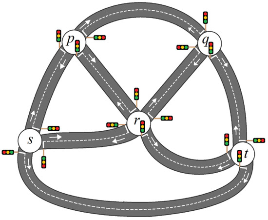
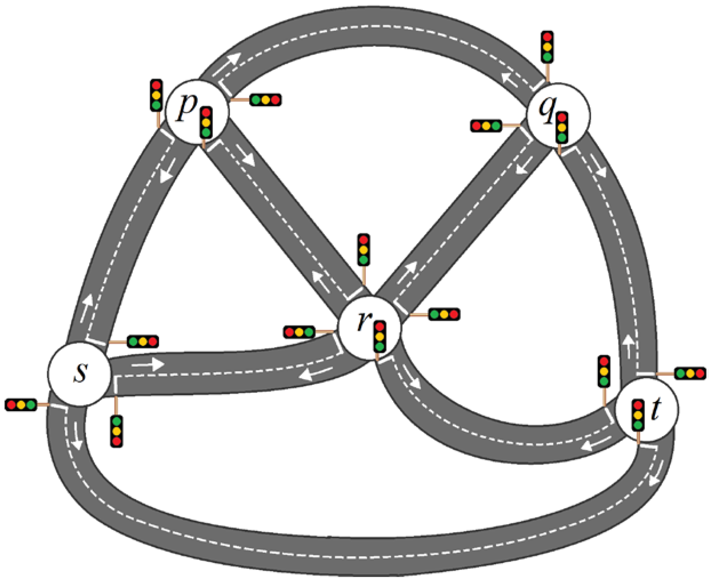
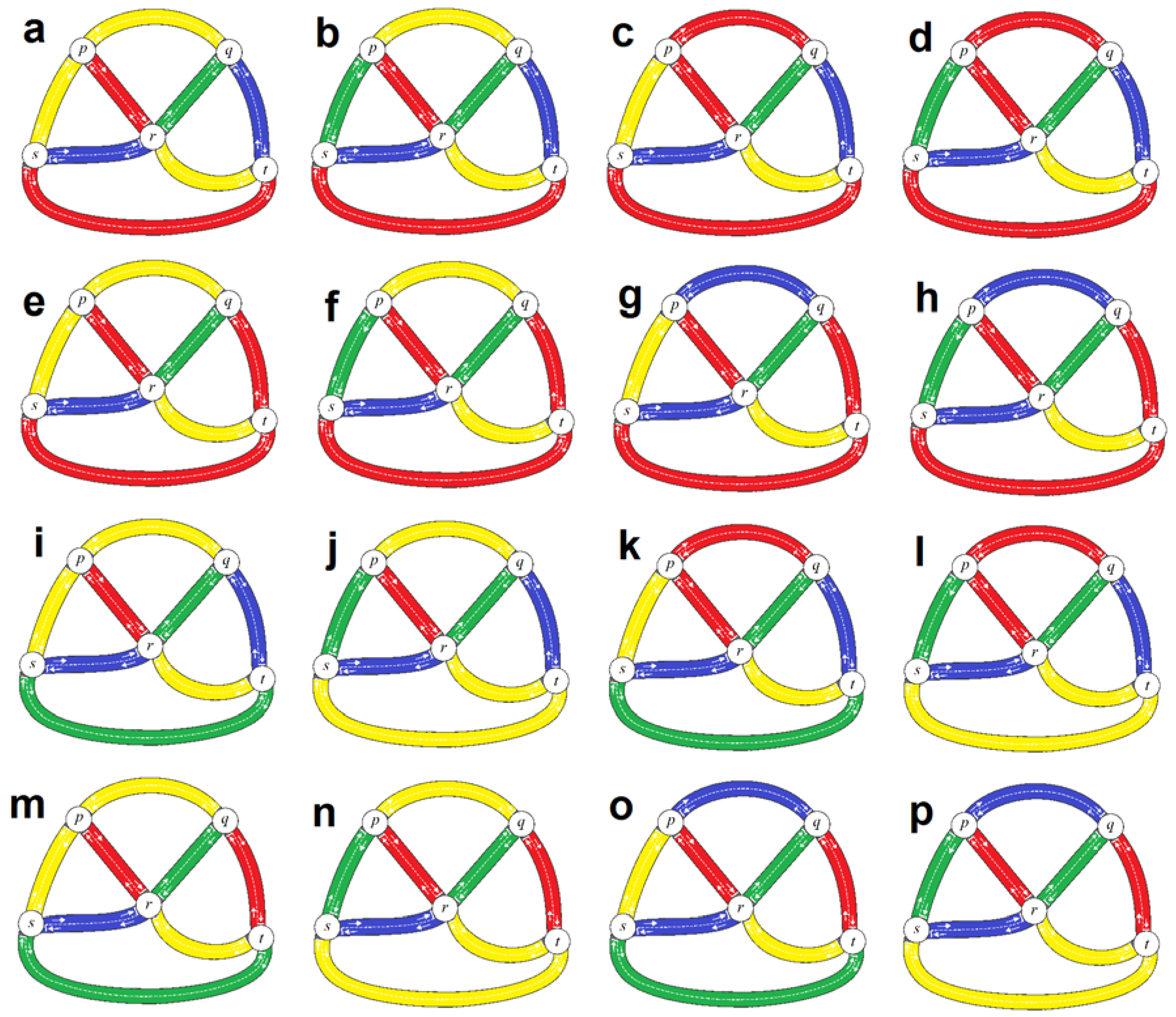
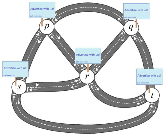
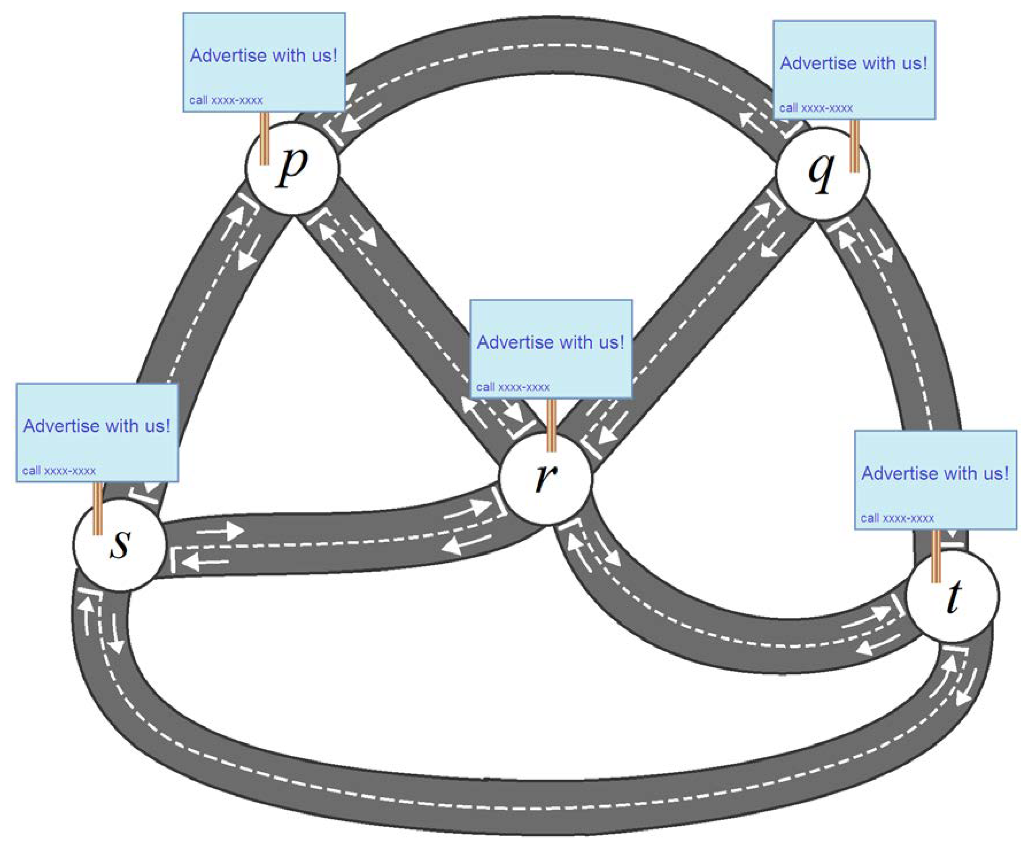
The regional government is concerned about the traffic entering a town through the roads, in the sense that if left unregulated, it can cause traffic jam within the town. As a result, traffic lights are to be built at the end of each road regulating the traffic entering a town, as shown in Figure 2. Note that the traffic lights only control the traffic entering a town, and no restriction is imposed by those traffic lights on those leaving a town, or driving along a road.

Figure 2. The traffic lights.

For any two roads with sufficiently high traffic entering a town, the traffic lights should be scheduled to allow for traffic from one road to enter at a time. Moreover, the traffic capacity of the town itself must be taken into account as well (i.e., larger town can accommodate more traffic).

The regional government understands that the amount of traffic on both sides of a given road is quite close. Thus, the traffic lights at both sides of a road will be operated simultaneously to provide an equal traffic flow rate on both sides of the road.

The regional government is taking very serious action to prevent the previous congested traffic from getting more worse; hence the volume of traffic entering a town will be considered significant enough, “even if it only reaches a seemingly low percentage…(S2)”of the traffic amount within that town.

On top of all these, the regional government is concerned about a very serious environmental issue—if too much traffic is entering a town at any instant, the atmosphere will not be capable of dispersing the increasing smog from the exhausts, causing air pollution within the town or even the entire region. The schedule of traffic lights are also intended to keep the total amount of traffic entering all of the towns below a threshold, which in turn must be set as low as possible without jeopardizing the flow of traffic.

4.2.2. The Corresponding Solution

In this example, $\zeta$ (see Definition 12) is hereby set to be $\frac{1}{5}$, in light of (S2). We now have the following:

$$\frac{1}{5}{t}_{{\breve{\sigma }}_0}\left(p\right)=0.05,\frac{1}{5}{t}_{{\breve{\sigma }}_0}\left(q\right)=0.03,\frac{1}{5}{t}_{{\breve{\sigma }}_0}\left(r\right)=0.04,\frac{1}{5}{t}_{{\breve{\sigma }}_0}\left(s\right)=0.016,\frac{1}{5}{t}_{{\breve{\sigma }.}_0}\left(t\right)=0.024.$$

(1)

$$\frac{4}{5}+\frac{1}{5}{f}_{{\breve{\sigma }}_0}\left(p\right)=0.92,\frac{4}{5}+\frac{1}{5}{f}_{{\breve{\sigma }}_0}\left(q\right)=0.96,\frac{4}{5}+\frac{1}{5}{f}_{{\breve{\sigma }}_0}\left(r\right)=0.90,\frac{4}{5}+\frac{1}{5}{f}_{{\breve{\sigma }}_0}\left(s\right)=0.96,\frac{4}{5}+\frac{1}{5}{f}_{{\breve{\sigma }.}_0}\left(t\right)=0.94.$$

(2)

By applying Definition 13 onto all of the outcomes of Table 2 and Table 3, Equations (1) and (2), we arrive at the output given in Table 4.

Table 2. Value of $t_{{\breve{\mu }}_0}\left(a,b\right)$.

	b	$\mathit{p}$	$\mathit{q}$	$\mathit{r}$	$\mathit{s}$	$\mathit{t}$
a
$p$		0	0.05	0.18	0.05	0
$q$		0.02	0	0.13	0	0.10
$r$		0.15	0.14	0	0.07	0.09
$s$		0.06	0	0.05	0	0.02
$t$		0	0.08	0.10	0.03	0

Table 3. Value of $f_{{\breve{\mu }}_0}\left(a,b\right)$.

	b	$\mathit{p}$	$\mathit{q}$	$\mathit{r}$	$\mathit{s}$	$\mathit{t}$
a
$p$		1	0.92	0.65	0.88	1
$q$		0.95	1	0.81	1	0.85
$r$		0.62	0.82	1	0.82	0.75
$s$		0.90	1	0.85	1	0.96
$t$		1	0.87	0.80	0.95	1

Table 4. $\frac{1}{5}$ strong incidence of $\left(a,b\right)$ towards $b$.

	b	$\mathit{p}$	$\mathit{q}$	$\mathit{r}$	$\mathit{s}$	$\mathit{t}$
a
$p$		False	True	True	True	False
$q$		False	False	True	False	True
$r$		True	True	False	True	True
$s$		True	False	True	False	False
$t$		False	True	True	True	False

From the third row of Table 4, it is clear that “at least (even if it can be done) four colors will be needed…(S3)”. We now perform a combinatorial search to find all of the possible ${\left[\frac{1}{5},4\right]}_{\mathfrak{U}}$-ECS of ${\mathcal{G}}_0$.

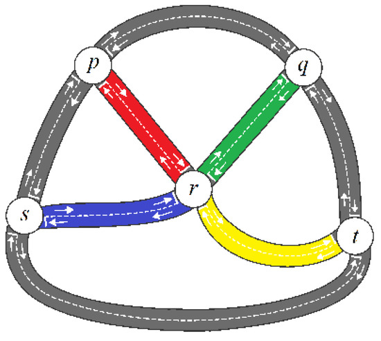
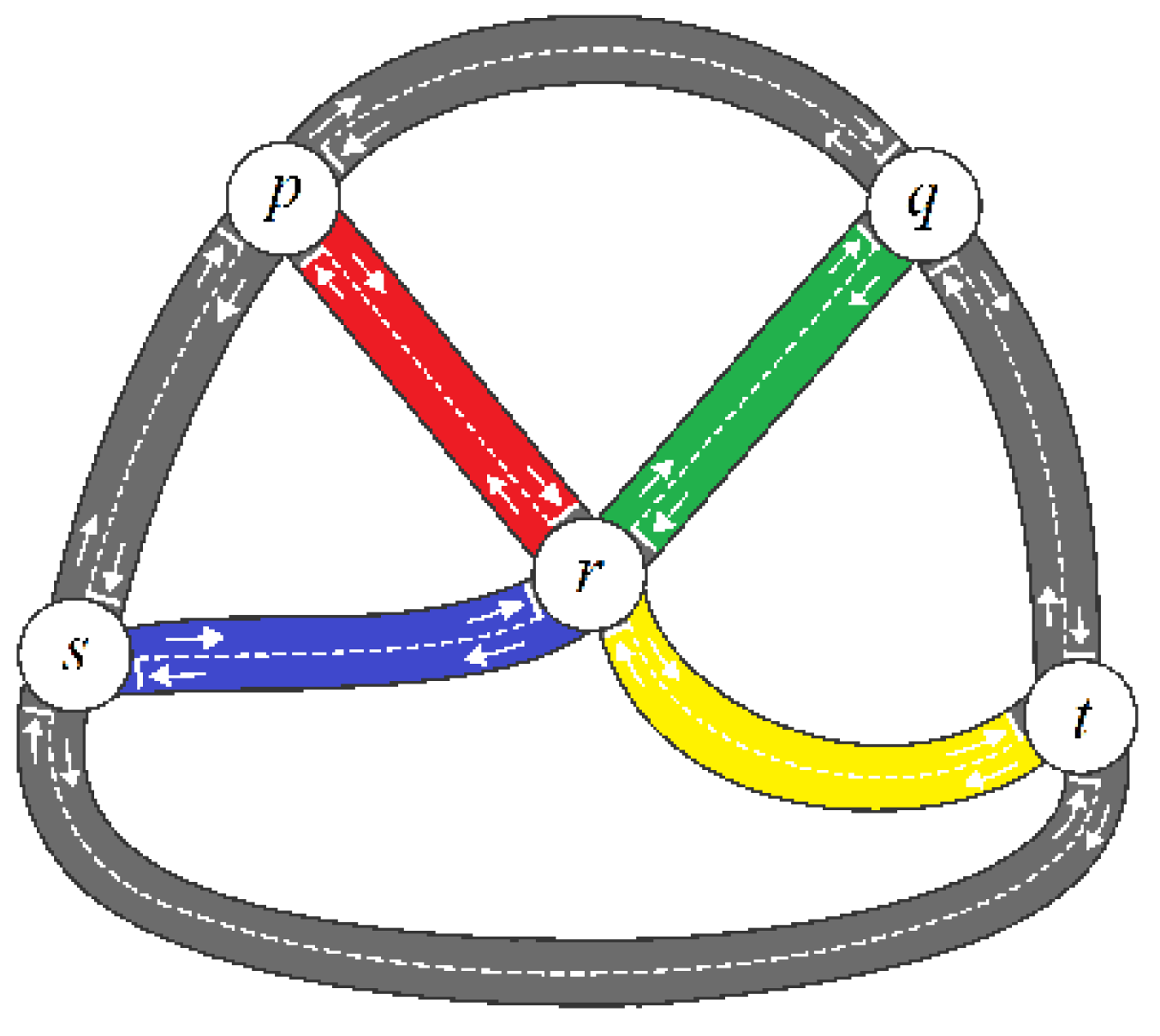
Firstly, as $\left(p,r\right)$, $\left(q,r\right)$, $\left(s,r\right)$, $\left(t,r\right)$ are all $\frac{1}{5}$ strong incident towards $r$, the roads $\left\{p,r\right\}$, $\left\{q,r\right\}$, $\left\{s,r\right\}$, $\left\{t,r\right\}$ must all be different colors. We shall fix the four colors to be red, greed, blue, and yellow, respectively, as shown in Figure 3.

Figure 3. The first four roads painted.

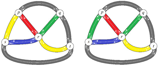
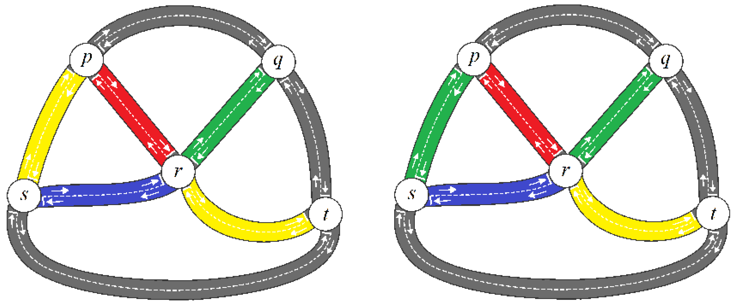
Note that $\left(p,s\right)$ and $\left(r,s\right)$ are both $\frac{1}{5}$ strong incident towards $s$. Furthermore, $\left(s,p\right)$ and $\left(r,p\right)$ are both $\frac{1}{5}$ strong incident towards $s$. The roads $\left\{p,r\right\}$, $\left\{s,r\right\}$, $\left\{p,s\right\}$ must all be different colors, this gives rise to two ways of coloring the road $\left\{p,s\right\}$, yellow or green (Figure 4).

Figure 4. Two ways to paint $\left\{p,s\right\}$.

However, $\left(q,t\right)$ and $\left(r,t\right)$ are both $\frac{1}{5}$ strong incident towards $t$. Furthermore, $\left(r,q\right)$ and $\left(t,q\right)$ are both $\frac{1}{5}$ strong incident towards $q$. As a result, the roads $\left\{q,r\right\}$, $\left\{t,r\right\}$, $\left\{q,t\right\}$ must all be different colors as well, and this gives rise to two ways of coloring the road $\left\{q,t\right\}$, red or blue. We now have four possible combinations thus far, as shown in Figure 5.

Figure 5. Two ways to paint $\left\{q,t\right\}$, which give rise to four ways to paint the first six roads.

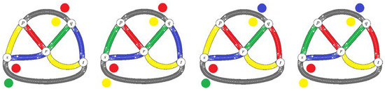
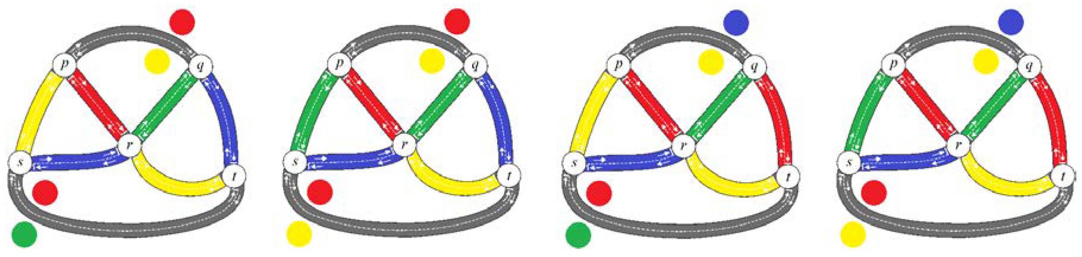
Note that $\left(t,s\right)$ is $\frac{1}{5}$ strong incident towards $s$, but $\left(s,t\right)$ is not $\frac{1}{5}$ strong incident towards $t$. Likewise, $\left(p,q\right)$ is $\frac{1}{5}$ strong incident towards $q$, but $\left(q,p\right)$ is not $\frac{1}{5}$ strong incident towards $p$. As a result, road $\left\{p,q\right\}$ must be different color from both $\left\{r,q\right\}$ and $\left\{t,q\right\}$, but it may share the same color as $\left\{p,r\right\}$ or $\left\{p,s\right\}$. Likewise, road $\left\{s,t\right\}$ must be different colors from both $\left\{r,s\right\}$ and $\left\{p,s\right\}$, but it may share the same color as $\left\{r,t\right\}$ or $\left\{t,q\right\}$. As a result, there will always be two ways to paint $\left\{p,q\right\}$, and there will also be two ways to paint $\left\{s,t\right\}$.

Moreover, $\left\{p,q\right\}$ and $\left\{s,t\right\}$ are not two neighbouring roads, thus $\left\{p,q\right\}$ can have the same color as $\left\{s,t\right\}$ (i.e., no restriction). The colors that can be used to do so are shown in Figure 6.

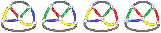
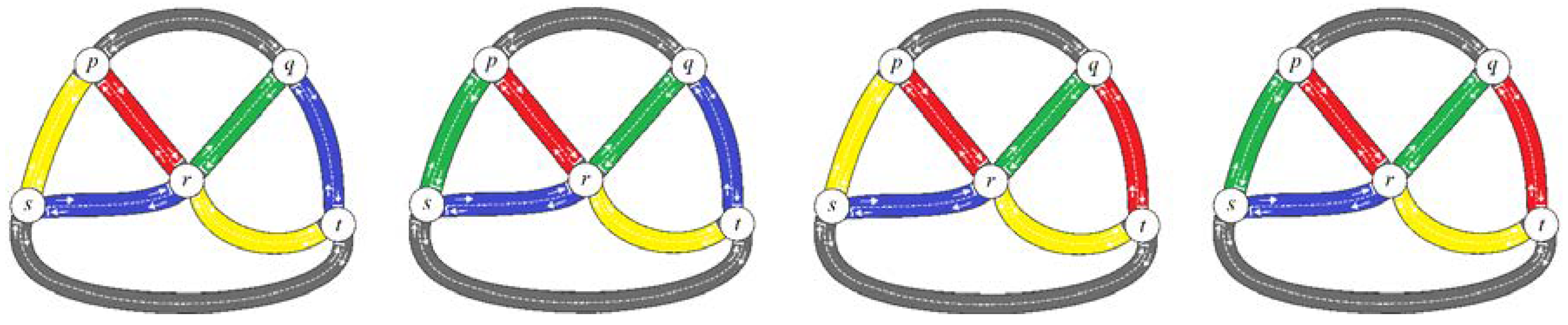
Figure 6. Each of the four ways of painting as shown in Figure 5 gives rise to four different ways of completing the coloring scheme.

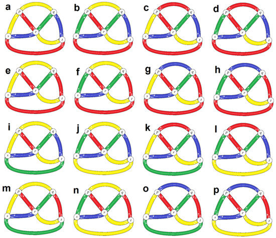
We now have altogether formed $4\times 4=16$ distinct ${\left[\frac{1}{5},4\right]}_{\mathfrak{U}}$-ECS of ${\mathcal{G}}_0$, as shown in Figure 7.

Figure 7. An illustration of all the sixteen ${\left[\frac{1}{5},4\right]}_{\mathfrak{U}}$-ECS() of ${\mathcal{G}}_0$ (mutual switching of colors are ignored).

In light of (S3), ${\mathcal{E}}_{\mathfrak{U}}^{\left[\frac{1}{5}\right]}\left({\mathcal{G}}_0\right)=4$ follows, and the sixteen ${\left[\frac{1}{5},4\right]}_{\mathfrak{U}}$-ECS of ${\mathcal{G}}_0$, are thus the sixteen ${\left[\frac{1}{5},\min \right]}_{\mathfrak{U}}$-ECS of ${\mathcal{G}}_0$.

As the total traffic entering all of the towns must be controlled, we should search the ${\left[\frac{1}{5},\min \right]}_{\mathfrak{U}}$-ECS with the lowest upper chromatic weight.

From Table 3, the value of 1−$f_{{\breve{\mu }}_0}\left(a,b\right)$ are deduced and shown in Table 5.

Table 5. Value of $1-f_{{\breve{\mu }}_0}\left(a,b\right)$.

	b	$\mathit{p}$	$\mathit{q}$	$\mathit{r}$	$\mathit{s}$	$\mathit{t}$
a
$p$		0	0.08	0.35	0.12	0
$q$		0.05	0	0.19	0	0.15
$r$		0.38	0.18	0	0.18	0.25
$s$		0.10	0	0.15	0	0.04
$t$		0	0.13	0.20	0.05	0

The maximum amount of ${\mathsf{\Phi }}_i\in${red, yellow, green, blue} by ${\mathrm{D}}_{\frac{1}{5},4}\in${a,b,c, …,p} on ${\mathcal{G}}_0$, and thus the upper chromatic weight of ${\mathrm{D}}_{\frac{1}{5},4}\in${a,b,c, …,p}, iscalculated as in Table 6, in accordance with Definition 21.

Table 6. The maximum amount of the four colors in the sixteen ${\left[\frac{1}{5},\min \right]}_{\mathfrak{U}}$ -ECS, and the upper chromatic weight of the sixteen ${\left[\frac{1}{5},\min \right]}_{\mathfrak{U}}$ -ECS.

	Red	Yellow	Green	Blue	Upper Chromatic Weight
A	0.82	0.80	0.37	0.61	0.82
B	0.82	0.58	0.59	0.61	0.82
C	0.95	0.67	0.37	0.61	0.95
D	0.95	0.45	0.59	0.61	0.95
E	1.10	0.80	0.37	0.33	1.10
F	1.10	0.58	0.59	0.33	1.10
G	1.10	0.67	0.37	0.46	1.10
H	1.10	0.45	0.59	0.46	1.10
I	0.73	0.80	0.46	0.61	0.80
J	0.73	0.67	0.59	0.61	0.73
K	0.86	0.67	0.46	0.61	0.86
L	0.86	0.54	0.59	0.61	0.86
M	1.01	0.80	0.46	0.33	1.01
N	1.01	0.67	0.59	0.33	1.01
O	1.01	0.67	0.46	0.46	1.01
P	1.01	0.54	0.59	0.46	1.01

As calculated, j is thus the ${\left[\frac{1}{5},\min \right]}_{\mathfrak{U}}$-ECS of ${\mathcal{G}}_0$ with the lowest upper chromatic weight.

4.2.3. A Practical Interpretation of the Results

Theoretically, the regional government can choose j, and by setting the traffic lights in each colored road taking turns to show green in 5 min. For example,

From 8:00:00 to 8:04:59 traffic lights in blue colored roads show green, others remain red.

From 8:05:00 to 8:09:59 traffic lights in green colored roads show green, others remain red.

From 8:10:00 to 8:14:59 traffic lights in red colored roads show green, others remain red.

From 8:15:00 to 8:19:59 traffic lights in yellow colored roads show green, others remain red.

The process then repeats for all of the subsequent intervals of 20 min. As mentioned, the traffic lights only control the traffic entering a town, and no restriction is imposed by those traffic lights on those leaving a town, or driving a long road.

4.3. Vertex Coloring

4.3.1. The Scenario

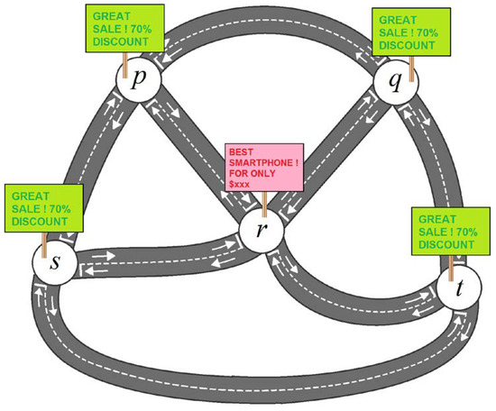
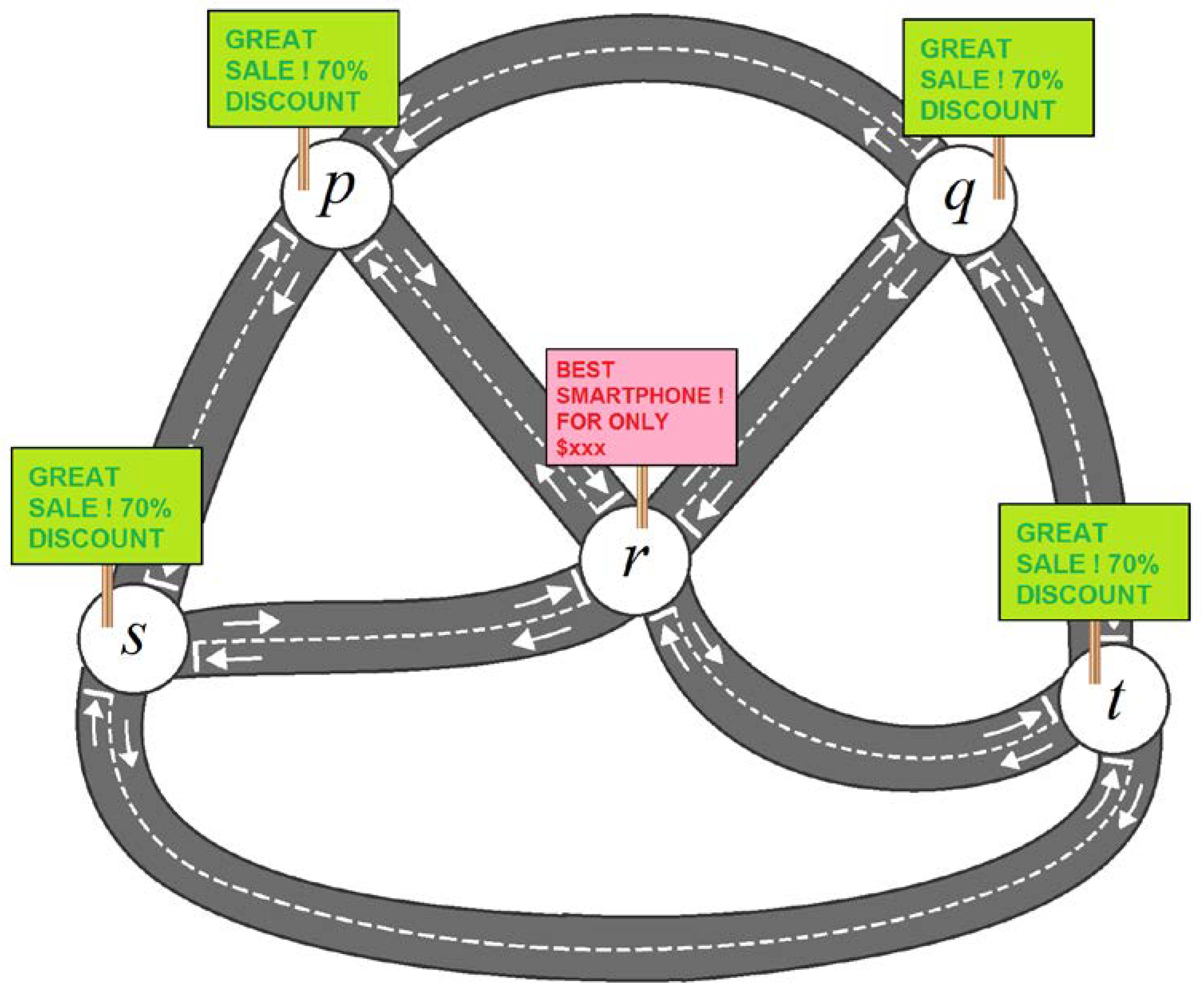
There is now another company that wants to advertise its product to the entire region. Because of budget constraint, the company can only afford a single kind of advertisement within a town (Figure 8).

Figure 8. The advertisement boards.

The company hopes that almost all of the people living in the entire region are able to see the advertisements, moreover, making more types of advertisement will lead to more job opportunities, particularly for the marketing and graphic designer team (i.e., cannot be too many types of advertisement). At the same time, the company still needs to advertise as many products as practically possible (i.e., cannot be too few types of advertisement) to generate the most venue. Thus, the company is looking at traffic pattern; if using two different advertisements on two towns, then all of the transports going between the two towns will still see both of them.

The company therefore decide to advertise two different kind of products in two different towns “only if a very substantial amount of mutual traffic flow…(S4)” exist between them. Moreover, the company must be sure that at least one of the advertisement can be seen by most, if not all, the people in the region.

4.3.2. The Corresponding Solution

In this example, $\lambda$ (see Definition 12) is hereby set to be $\frac{3}{4}$, in light of (S4).

$$\frac{3}{4}{t}_{{\breve{\sigma }}_0}\left(p\right)=0.1875,\frac{3}{4}{t}_{{\breve{\sigma }}_0}\left(q\right)=0.1125,\frac{3}{4}{t}_{{\breve{\sigma }}_0}\left(r\right)=0.15,\frac{3}{4}{t}_{{\breve{\sigma }}_0}\left(s\right)=0.06,\frac{3}{4}{t}_{{\breve{\sigma }.}_0}\left(t\right)=0.09.$$

(3)

$$\frac{1}{4}+\frac{3}{4}{f}_{{\breve{\sigma }}_0}\left(p\right)=0.70,\frac{1}{4}+\frac{3}{4}{f}_{{\breve{\sigma }}_0}\left(q\right)=0.85,\frac{1}{4}+\frac{3}{4}{f}_{{\breve{\sigma }}_0}\left(r\right)=0.625,\frac{1}{4}+\frac{3}{4}{f}_{{\breve{\sigma }}_0}\left(s\right)=0.85,\frac{1}{4}+\frac{3}{4}{f}_{{\breve{\sigma }.}_0}\left(t\right)=0.775.$$

(4)

We then proceed with the computation of $t_{{\breve{\mu }}_0}\left(a,b\right)\wedge t_{{\breve{\mu }}_0}\left(b,a\right)$, $f_{{\breve{\mu }}_0}\left(a,b\right)\vee f_{{\breve{\mu }}_0}\left(b,a\right)$, $\frac{3}{4}\left(t_{{\breve{\sigma }}_0}\left(a\right)\wedge t_{{\breve{\sigma }}_0}\left(b\right)\right)$, and $\frac{1}{4}+\frac{3}{4}\left(f_{{\breve{\sigma }}_0}\left(a\right)\vee f_{{\breve{\sigma }}_0}\left(b\right)\right)$.

By applying Definition 12 to all of the outcomes of Table 7, Table 8, Table 9 and Table 10, we arrive at the output, as shown in Table 11.

Table 7. Values of $t_{{\breve{\mu }}_0}\left(a,b\right)\wedge t_{{\breve{\mu }}_0}\left(b,a\right)$.

	b	$\mathit{p}$	$\mathit{q}$	$\mathit{r}$	$\mathit{s}$	$\mathit{t}$
a
$p$		0	0.02	0.15	0.05	0
$q$		0.02	0	0.13	0	0.08
$r$		0.15	0.13	0	0.05	0.09
$s$		0.05	0	0.05	0	0.02
$t$		0	0.08	0.09	0.02	0

Table 8. Values of $f_{{\breve{\mu }}_0}\left(a,b\right)\vee f_{{\breve{\mu }}_0}\left(b,a\right)$ .

	b	$\mathit{p}$	$\mathit{q}$	$\mathit{r}$	$\mathit{s}$	$\mathit{t}$
a
$p$		1	0.95	0.65	0.90	1
$q$		0.95	1	0.82	1	0.87
$r$		0.65	0.82	1	0.85	0.80
$s$		0.90	1	0.85	1	0.96
$t$		1	0.87	0.80	0.96	1

Table 9. Values of $\frac{3}{4}\left(t_{{\breve{\sigma }}_0}\left(a\right)\wedge t_{{\breve{\sigma }}_0}\left(b\right)\right)$.

	b	$\mathit{p}$	$\mathit{q}$	$\mathit{r}$	$\mathit{s}$	$\mathit{t}$
a
$p$		0.1875	0.1125	0.15	0.06	0.09
$q$		0.1125	0.1125	0.1125	0.06	0.09
$r$		0.15	0.1125	0.15	0.06	0.09
$s$		0.06	0.06	0.06	0.06	0.06
$t$		0.09	0.09	0.09	0.06	0.09

Table 10. Values of $\frac{1}{4}+\frac{3}{4}\left(f_{{\breve{\sigma }}_0}\left(a\right)\vee f_{{\breve{\sigma }}_0}\left(b\right)\right)$.

	b	$\mathit{p}$	$\mathit{q}$	$\mathit{r}$	$\mathit{s}$	$\mathit{t}$
a
$p$		0.7	0.85	0.7	0.85	0.775
$q$		0.85	0.85	0.85	0.85	0.85
$r$		0.7	0.85	0.635	0.85	0.775
$s$		0.85	0.85	0.85	0.85	0.85
$t$		0.775	0.85	0.775	0.85	0.775

Table 11. Mutual $\frac{3}{4}$ -strong adjacency of $a$ and $b$.

	b	$\mathit{p}$	$\mathit{q}$	$\mathit{r}$	$\mathit{s}$	$\mathit{t}$
a
$p$		False	False	True	False	False
$q$		False	False	True	False	False
$r$		True	True	False	False	False
$s$		False	False	False	False	False
$t$		False	False	False	False	False

Thus, it is found that the $\left(r,q\right)$, $\left(q,r\right)$, $\left(r,p\right)$, $\left(p,r\right)$ have a very high flow of traffic. Indeed, compared to $p$ and $q$, the company should put out a different kind of advertisement in $r$. Hence, “at least two advertisements…(S5)” should be made.

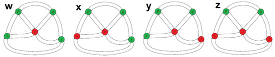
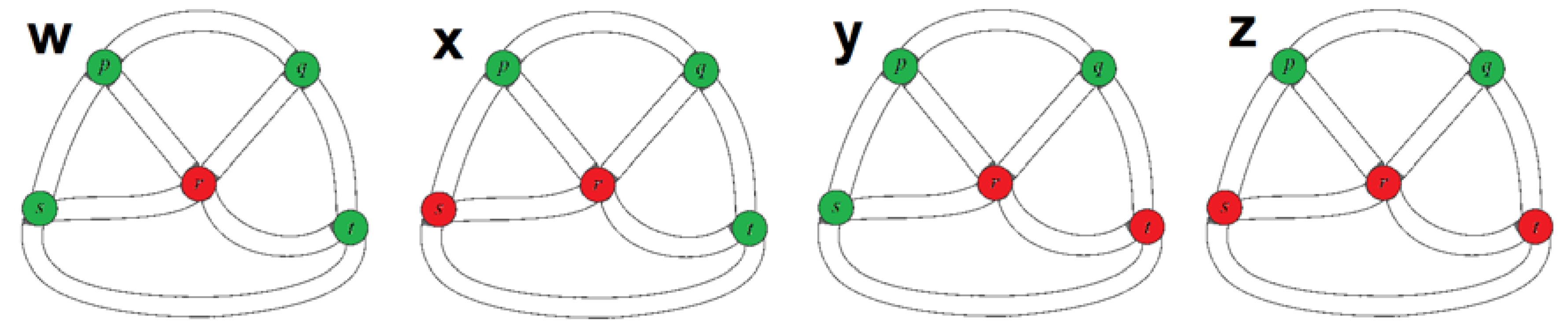
We shall now search for all of the ${\left[\frac{3}{4},2\right]}_{\mathfrak{U}}$-VCS of ${\mathcal{G}}_0$.We shall use the color red and green.

Firstly, we shall fix $r$ red and $p$, $q$ to be green. As there are no restrictions on the color of $s$ and $t$, there are thus four ways of painting the vertices. As a result, there are altogether four ${\left[\frac{3}{4},2\right]}_{\mathfrak{U}}$-VCS of ${\mathcal{G}}_0$, as illustrated in Figure 9.

Figure 9. An illustration of all the four ${\left[\frac{3}{4},2\right]}_{\mathfrak{U}}$-VCS of ${\mathcal{G}}_0$ (mutual switching of colors are ignored).

In light of (S5), ${\mathcal{X}}_{\mathfrak{U}}^{\left[\frac{3}{4}\right]}\left({\mathcal{G}}_0\right)=2$ follows, and the four ${\left[\frac{3}{4},2\right]}_{\mathfrak{U}}$-VCS of ${\mathcal{G}}_0$ are thus the four ${\left[\frac{3}{4},\min \right]}_{\mathfrak{U}}$-VCS of ${\mathcal{G}}_0$.

As one of the advertisements must be seen by many, we should search the ${\left[\frac{3}{4},\min \right]}_{\mathfrak{U}}$-VCS with the highest lower chromatic weight.

Note that $t_{{\breve{\sigma }}_0}\left(p\right)=0.25>0.20=t_{{\breve{\sigma }}_0}\left(r\right)$. In accordance with Definition 18, for the lower chromatic weight to be the highest, $s$ and $t$ must follow the same color as $p$. w is thus the ${\left[\frac{3}{4},\min \right]}_{\mathfrak{U}}$-VCS of ${\mathcal{G}}_0$ with the highest lower chromatic weight and should be chosen by the company. Figure 10 provides an illustration for w.

Figure 10. The way to put up the advertisements following w.

4.3.3. Practical Interpretation of the Results

Thus, with the very high and mutual traffic flow between $p$ and $q$ with $r$, many people who live/work at $r$ will still notice the green advertisement “GREAT SALE 70% DISCOUNT” as they drive to $p$ or $q$.

Thus, even in the case of zero traffic between $r$ and any of the other four towns within a given day, 50–80% of the drivers will still notice the green advertisement, the remaining 20–50% of the drivers will still see the red advertisement “BEST SMARTPHONE FOR ONLY $xxx”. This is a worst-case scenario, and such a scenario is extremely unlikely, as 0% is out of the range of the values in Table 1, which is the result of an observation from 500 consecutive days, not to mention the abundance of the delivery and GrabCar service from $r$.

Therefore, more profit can be expected than using only one advertisement for all of the towns, as some people get to see two different advertisements instead of one, increasing their chances of buying the company’s products.

In this paper, we have used the concept of vague graphs to represent real-life problems, and we also introduce some novel definitions of vertex and edge coloring for simple vague graphs. Those concepts are used to solve traffic flow management and the selection of advertisement spots that will optimize the visibility of the advertisements. The major strength of the paper is that the proposed vertex and edge coloring model of vague graph, while being practically simple, has the flexibility to manage the uncertainty of real-life problems and effectively solve traffic flow management and the selection of advertisement spots problems. The effectiveness of our proposed model was described by working out an illustrating application. However, in the future, some theorems and corollaries interpreting the significance of edge coloring could be written, and we also try to apply our proposed idea to solve other real life problems [27,28,29,30,31,32,33,34,35,36,37,38,39,40].

5. Conclusions

This paper introduced some novel definitions of vertex and edge coloring for simple vague graphs. The concepts that were introduced include the strong vertex chromatic number, and the $\lambda$-strong and $\lambda$-strong minimal vague vertex coloring scheme, as well as the strong edge chromatic number, and $\lambda$-strong and $\lambda$-strong minimal edge coloring scheme. The vertex membership values of the vague graphs were used together with the different coloring methods, based on the membership values. The applicability and practical aspects of all of the concepts and definitions introduced here were demonstrated using two scenarios related to traffic flow and advertising. The edge coloring for vague graphs were used to model traffic light positioning and scheduling to optimize the traffic flow in a town setting, whereas the vertex coloring were used to model a problem involving the selection of the best place for a company to place its advertisement. It was clearly demonstrated that our proposed methods of vertex and edge coloring for vague graphs are able to model these commonly encountered daily problems in an efficient manner. It was clearly demonstrated that our proposed methods of vertex and edge coloring for vague graphs are able to model these commonly encountered daily problems in an efficient manner.

References

- Rosenfeld, A. Fuzzy graphs. In Fuzzy Sets and Their Applications; Zadeh, L.A., Fu, K.S., Shimura, M., Eds.; Academic Press: New York, NY, USA, 1975; pp. 77–95. [Google Scholar]
- Eslahchi, C.; Onagh, B.N. Vertex strength of fuzzy graphs. Int. J. Math. Math. Sci. 2006, 2006, 43614. [Google Scholar] [CrossRef] [Scilit]
- Mordeson, J.N.; Peng, C.S. Operations on fuzzy graphs. Inf. Sci. 1994, 79, 159–170. [Google Scholar] [CrossRef] [Scilit]
- Mathew, J.K.; Mathew, S. Some special sequences in fuzzy graphs. Fuzzy Inf. Eng. 2016, 8, 31–40. [Google Scholar] [CrossRef] [Scilit]
- Lavanya, S.; Sattanathan, R. Fuzzy total coloring of fuzzy graphs. Int. J. Inf. Technol. Knowl. Manag. 1998, 2, 37–39. [Google Scholar]
- Jaiswal, R.; Rai, S. Application of fuzzy graph coloring in traffic light problem. Int. J. Innov. Res. Sci. Eng. Technol. 2016, 5, 6950–6955. [Google Scholar]
- Samanta, S.; Pramanik, T.; Pal, M. Fuzzy coloring of fuzzy graphs. Afr. Mat. 2016, 27, 37–50. [Google Scholar] [CrossRef] [Scilit]
- Kishore, A.; Sunitha, M.S. Chromatic number of resultant of fuzzy graphs. Fuzzy Inf. Eng. 2016, 8, 229–235. [Google Scholar] [CrossRef] [Scilit]
- Ghorai, G.; Pal, M. On some operations and density of m-polar fuzzy graphs. Pac. Sci. Rev. A Nat. Sci. Eng. 2015, 17, 14–22. [Google Scholar] [CrossRef] [Scilit]
- Ghorai, G.; Pal, M. Some properties of m-polar fuzzy graphs. Pac. Sci. Rev. A Nat. Sci. Eng. 2016, 18, 38–46. [Google Scholar] [CrossRef] [Scilit]
- Ghorai, G.; Pal, M. A study on m-polar fuzzy planar graphs. Int. J. Comput. Sci. Math. 2016, 7, 283–292. [Google Scholar] [CrossRef] [Scilit]
- Ghorai, G.; Pal, M. Faces and dual of m-polar fuzzy planar graphs. J. Intell. Fuzzy Syst. 2016, 31, 2043–2049. [Google Scholar] [CrossRef] [Scilit]
- Ghorai, G.; Pal, M. Some isomorphic properties of m-polar fuzzy graphs with applications. SpringerPlus 2016, 5. [Google Scholar] [CrossRef] [Scilit] [PubMed]
- Ghorai, G.; Pal, M. A note on “Regular bipolar fuzzy graphs” Neural Computing and Applications 21(1) (2012) 197–205. Neural Comput. Appl. 2016. [Google Scholar] [CrossRef] [Scilit]
- Gau, W.L.; Buehrer, D.J. Vague sets. IEEE Trans. Syst. Man Cybern. 1993, 23, 610–614. [Google Scholar] [CrossRef] [Scilit]
- Akram, M.; Feng, F.; Sarwar, S.; Jun, Y.B. Certain types of vague graphs. UPB Sci. Bull. Ser. A 2014, 76, 141–154. [Google Scholar]
- Borzooei, R.A.; Rashmanlou, H. New concepts on vague graphs. Int. J. Mach. Learn. Cybern. 2017, 8, 1081–1092. [Google Scholar] [CrossRef] [Scilit]
- Talebi, A.A.; Rashmanlou, H.; Mehdipoor, N. Isomorphism on vague graphs. Ann. Fuzzy Math. Inform. 2013, 6, 575–588. [Google Scholar]
- Borzooei, R.A.; Rashmanlou, H.; Mathew, S. Some new concepts on highly irregular vague graphs. In Proceedings of the 4th IEEE Iranian Joint Congress on Fuzzy and Intelligent Systems (CFIS), Zahedan, Iran, 9–11 September 2015; pp. 1–4. [Google Scholar]
- Samanta, S.; Pal, M.; Rashmanlou, H.; Borzooei, R.A. Vague graphs and strengths. J. Intell. Fuzzy Syst. 2016, 30, 3675–3680. [Google Scholar] [CrossRef] [Scilit]
- Ghorai, G.; Pal, M. Regular product vague graphs and product vague line graphs. Cogent Math. 2016, 3, 1213214. [Google Scholar] [CrossRef] [Scilit]
- Rashmanlou, H.; Samanta, S.; Pal, M.; Borzooei, R.A. A study on vague graphs. SpringerPlus 2016, 5, 1234–1245. [Google Scholar] [CrossRef] [Scilit] [PubMed]
- Darabian, E.; Borzooei, R.A.; Rashmanlou, H.; Azadi, M. New concepts of regular and (highly) irregular vague graphs with applications. Fuzzy Inf. Eng. 2017, 9, 161–179. [Google Scholar]
- Borzooei, R.A.; Rashmanlou, H. More results on vague graphs. UPB Sci. Bull. Ser. A 2016, 78, 109–122. [Google Scholar]
- Borzooei, R.A.; Darabian, E.; Rashmanlou, H. Strong domination numbers of vague graphs with applications. Appl. Math. E-Notes 2016, 16, 251–267. [Google Scholar]
- Solairaju, A.; Robinson, P.J.; Lenin, T. Applications of transforming vague sets into fuzzy sets for knowledge management. Int. J. Comput. Algorithm 2013, 2, 430–439. [Google Scholar]
- Phuong, P.T.M.; Thong, P.H.; Son, L.H. Theoretical analysis of picture fuzzy clustering: Convergence and property. J. Comput. Sci. Cybern. 2018, 1, 17–32. [Google Scholar] [CrossRef] [Scilit]
- Jha, S.; Kumar, R.; Chatterjee, J.M.; Khari, M.; Yadav, N.; Smarandache, F. Neutrosophic soft set decision making for stock trending analysis. Evolv. Syst. 2018, 1–7. [Google Scholar] [CrossRef] [Scilit]
- Ngan, R.T.; Son, L.H.; Cuong, B.C.; Ali, M. H-max distance measure of intuitionistic fuzzy sets in decision making. Appl. Soft Comput. 2018, 69, 393–425. [Google Scholar] [CrossRef] [Scilit]
- Giap, C.N.; Son, L.H.; Chiclana, F. Dynamic structural neural network. J. Intell. Fuzzy Syst. 2018, 34, 2479–2490. [Google Scholar] [CrossRef] [Scilit]
- Ali, M.; Son, L.H.; Thanh, N.D.; Van Minh, N. A neutrosophic recommender system for medical diagnosis based on algebraic neutrosophic measures. Appl. Soft Comput. 2017. [Google Scholar] [CrossRef] [Scilit]
- Ali, M.; Son, L.H.; Khan, M.; Tung, N.T. Segmentation of dental X-ray images in medical imaging using neutrosophic orthogonal matrices. Expert Syst. Appl. 2018, 91, 434–441. [Google Scholar] [CrossRef] [Scilit]
- Ali, M.; Dat, L.Q.; Son, L.H.; Smarandache, F. Interval complex neutrosophic set: Formulation and applications in decision-making. Int. J. Fuzzy Syst. 2018, 20, 986–999. [Google Scholar] [CrossRef] [Scilit]
- Son, L.H.; Tuan, T.M.; Fujita, H.; Dey, N.; Ashour, A.S.; Ngoc, V.T.N.; Chu, D.T. Dental diagnosis from X-ray images: An expert system based on fuzzy computing. Biomed. Signal Process.Control 2018, 39, 64–73. [Google Scholar] [CrossRef] [Scilit]
- Nguyen, G.N.; Son, L.H.; Ashour, A.S.; Dey, N. A survey of the state-of-the-arts on neutrosophic sets in biomedical diagnoses. Int. J. Mach. Learn. Cybern. 2017, 1–13. [Google Scholar] [CrossRef] [Scilit]
- Ngan, R.T.; Ali, M.; Son, L.H. δ-equality of intuitionistic fuzzy sets: A new proximity measure and applications in medical diagnosis. Appl. Intell. 2018, 48, 499–525. [Google Scholar] [CrossRef] [Scilit]
- Ali, M.; Son, L.H.; Deli, I.; Tien, N.D. Bipolar neutrosophic soft sets and applications in decision making. J. Intell. Fuzzy Syst. 2017, 33, 4077–4087. [Google Scholar] [CrossRef] [Scilit]
- Thanh, N.D.; Ali, M.; Son, L.H. A novel clustering algorithm in a neutrosophic recommender system for medical diagnosis. Cogn. Comput. 2017, 9, 526–544. [Google Scholar] [CrossRef] [Scilit]
- Son, L.H.; Viet, P.V.; Hai, P.V. Picture inference system: A new fuzzy inference system on picture fuzzy set. Appl. Intell. 2017, 46, 652–669. [Google Scholar] [CrossRef] [Scilit]
- Son, L.H.; Tien, N.D. Tune up fuzzy C-means for big data: Some novel hybrid clustering algorithms based on initial selection and incremental clustering. Int. J. Fuzzy Syst. 2017, 19, 1585–1602. [Google Scholar] [CrossRef] [Scilit]
© 2018 by the authors. Licensee MDPI, Basel, Switzerland. This article is an open access article distributed under the terms and conditions of the Creative Commons Attribution (CC BY) license (http://creativecommons.org/licenses/by/4.0/).