CRCM: A New Combined Data Gathering and Energy Charging Model for WRSN

Abstract

With the development of wireless sensor networks (WSNs), the problem about how to increase the lifecycle of the WSNs is always a hot discussion point, and some researchers have devoted to the ‘energy saving’ to decrease the energy consumption of the sensor nodes by different algorithms. However, the fundamental technique is ‘energy acquiring’ for the battery which can solve the limited capacity problem. In this paper, we study the data gathering and energy charging by a mobile charger (MC) at the same time that most energy consumption can be saved by short communication distance. We have named this as the recharging model-combined recharging and collecting data model on-demand (CRCM). Firstly, the hexagon-based (HB) algorithm is proposed to sort all sensor nodes in the region to make data collecting and energy charging work at the same time. Then we consider both residual energy and geographic position (REGP) of the sensor node to calculate the priority of each cluster. Thirdly, the dynamic mobile charger (DMC) algorithm is proposed to calculate the number of MCs to make sure no sensor node will die in each charging queue. Finally, the simulations show that our REGP algorithm is better than Earliest Deadline First (EDF) and Nearest-Job-Next with Preemption (NJNP), and the DMC plays well when the number of sensor nodes increase.

1. Introduction

Wireless sensor networks (WSNs) are used to monitor different environmental parameters in different domains, such as the military, medical treatment, and so on [1,2,3]. Sensor nodes are deployed randomly in an area to sense environmental parameters, such as temperature, humidity, and light. After collecting data, sensor nodes need to deliver it to the sink in each cycle. However, since the sensor nodes cannot be recharged, in general, the lifetime of the WSNs is limited by the battery capacity of the sensor nodes.

Many researchers have researched some effective approaches for prolonging the lifetime of the network. Some researchers focused on reducing the energy consumption of the battery, but the limited capacity of the battery restricts the lifetime of WSNs eventually. Other researchers have considered rechargeable batteries, the WSNs being updated to a wireless rechargeable sensor network (WRSN). To replenish energy to the batteries, the paramount consideration is the nature of the energy, such as solar energy, thermal energy, and wind energy [4]. Though the lifetime of the WRSN is obviously prolonged, with the unstable state of the external condition and low charging efficiency, sensor nodes could still exhaust their energy at any time. This scheme cannot actually solve the limited energy problem of the sensor nodes.

Since the nature of the energy cannot solve the charging problem utterly, another technology called wireless power transfer (WPT) [5,6,7] was introduced into WRSN. WPT technology is a hot topic in charging mobile devices, electric vehicles, and now in WRSN [8,9,10,11,12]. WPT can provide high charging efficiency over a short distance, the mobile charger (MC) carries a certain amount of energy and departs from the sink station to charge all sensor nodes [13,14]. Thus, a new problem about how to schedule the charging path of MC came into being. An algorithm based on the distance called Nearest-Job-Next with Preemption (NJNP) is a typical method to solve the problem [15]. However, due to not considering the energy consumption of each sensor node, the sensor node with high consumption can easily die during the whole process.

With the increasing quantity of sensor nodes, one MC still cannot satisfy all the sensor nodes in a charging cycle [16], so another problem about the least number of MCs is worth exploring. Dai and Kar have proposed an algorithm to minimize the number of MCs [17,18]. How to improve the charging efficiency is the key and, at the same time, clustering the sensor nodes in the region is of great importance with the increasing number of sensor nodes. Lin has studied nonoverlapping clusters, meaning the clusters in the region are separated from each other [19].

In this paper, we study the on-demand charging WRSN with multi-MCs [20]. The MCs only worked when the sensor nodes have to send recharging requests. There were several clusters in the WRSN. The MC was applied to a cluster containing sensor nodes which needed to be charged, and the MC can charge several sensor nodes at the same time. The contributions in this paper are as follows:

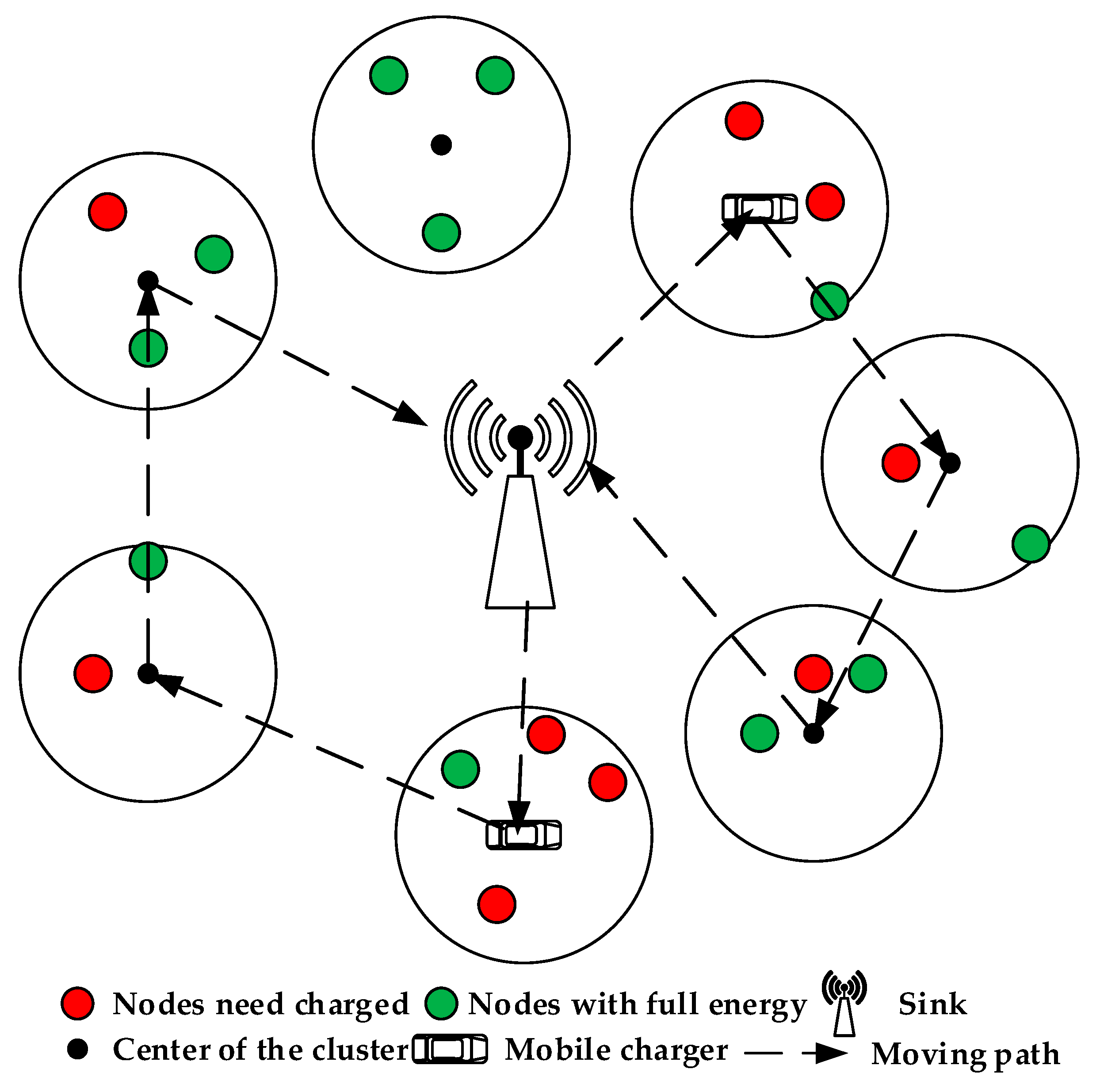
• To reduce the energy consumption to the largest extent, we consider the MC as a moving sink to gather sensing data from sensor nodes when charging them. A new recharging model, combined recharging and collecting data model on-demand (CRCM), was established in which the MC will recharge the on-demand sensor nodes and collect all of the data of the sensor nodes in the cluster at the same time.
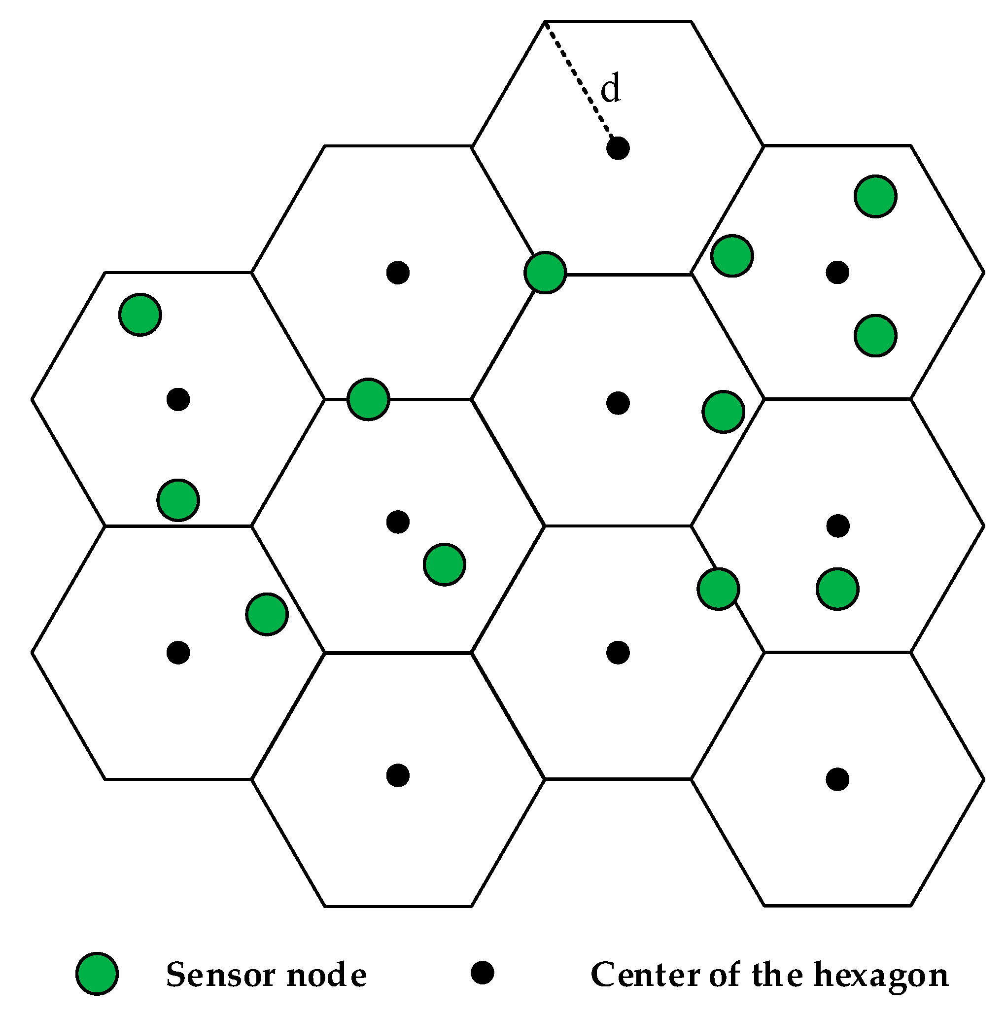
• To establish the CRCM, we have considered the hexagon-based [21] (HB) algorithm to sort all sensor nodes into different clusters. While NJNP cannot satisfy the scheduler with high charging efficiency to structure the charging path, we then consider both the residual energy and geographic position of each sensor node, the REGP algorithm is proposed to calculate the priority of each cluster, and the charging queue is ultimately established.
• In a large WRSN, we have also considered the multi-MC’s algorithm to adapt the increasing quantity of sensor nodes. To make sure no sensor nodes exhaust their energy while waiting for the next charging cycle, we have calculated the longest cycle time a MC can serve. The DMC algorithm is subsequently raised to solve the least number of MCs problem.
• The remainder of this paper is constituted as follows: in Section 2, we have discussed the related works about previous studies and experiments of WPT; in Section 3 we have shown the system model and three algorithms to solve the problems; then some simulations have been realized to compare each parameter to Earliest Deadline First (EDF) [22] and NJNP in Section 4; and, finally, we conclude this paper in Section 5.

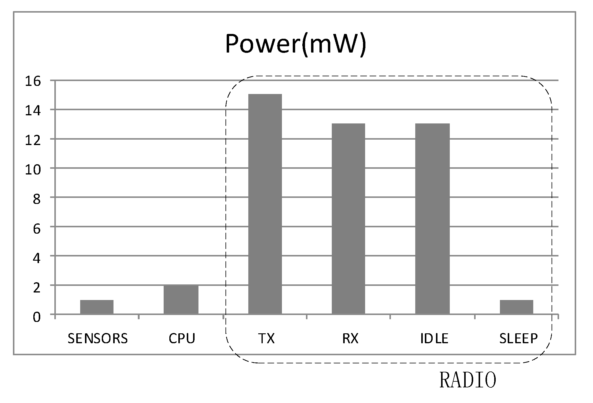
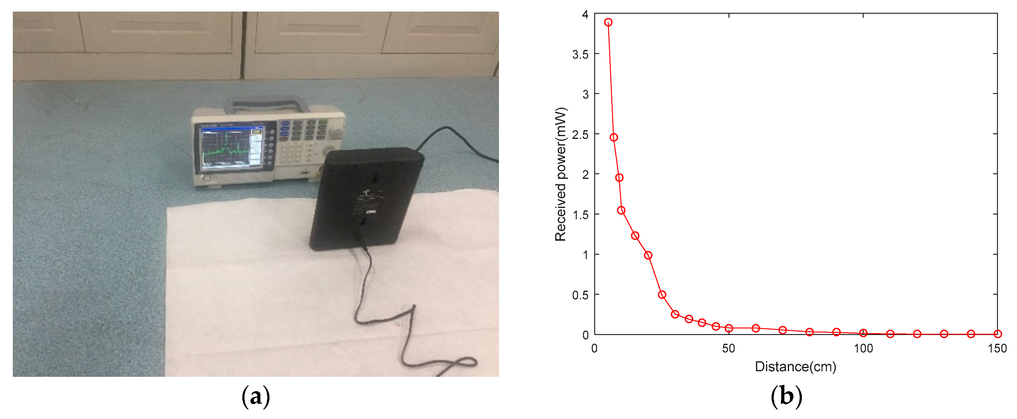
2. Related Works

To prolong the lifecycle of the network, two methods are supplied as ‘energy saving’ and ‘energy acquiring’. ‘Energy saving’ is the most direct approach. Sensor nodes can be alive and turned off to reduce the energy consumption, because not all the sensor nodes need to be alive for the WSNs to be functional [23]. The selected sensor nodes can be alive to form a connected wireless network, and the inactive sensor nodes can be turned off to prolong the lifecycle of the WSNs. Liu has proposed an algorithm called distributed cooperative communication nodes control (DCCNC) to achieve higher reliability communication and longer network lifetime [24]. They have proposed an algorithm to determine the appropriate number of sensor nodes to participate in the cooperative communication and, as a result, the resource is constrained.

In ‘energy acquiring’ aspect, Yang has used the solar energy to avoid battery exhaustion as well as maximizing the per-node utility [25]. To adapt the time-varying solar energy, the energy monitoring and prediction is also very important by energy-aware support. With the development of WPT, MC carries certain energy to travel to different sensor nodes with an optimal path. Xie has an overall consideration about the traveling path, stop points, charging schedule and the flow routing [26]. The charging path is optimized by the stopping points comparing to stopping at the location of sensor node with the shortest traveling distance.

However, data gathering and energy charging have always been discussed separately in recent years, Hu and Wang have studied the optimization of charging and data collection in a WRSN, and they have solved the problem about how to allocate the insufficient energy to the sensor nodes and deciding their corresponding data sensing rates [27]. Data gathering and energy charging can be replenished by MCs. Liu has proposed novel methods to distribute the sensor nodes, and also calculated the number of MCs [28]. In this paper, we consider the energy charging and data gathering at the same time by a MC [29,30,31]. With the data collecting by MC, the energy consumption of a sensor node can be decreased significantly.

Figure 1 shows the energy consumption of a sensor in the whole process. We can see the transport and receiving modules consume the most of the energy, the idle listening module also belongs to the communication part, and the energy consumption of communication follows the formula $E=k{d}^n(2<n<4)$, the parameter $n$ is influenced by the communication distance, i.e., when the communication distance is long, the parameter $n$ will be also larger, and, meanwhile, the communicating consumption of the sensor node will increase [32,33].

The TX91501 (Powercast, 620 Alpha Drive, Pittsburgh, PA, 15238, USA) is a typical charging equipment produced by Powercaster. In order to study the WPT efficiency of TX91501 [34], we have performed an experiment to contrast the efficiency of different distance. With the change of the distance between the TX91501 and the spectrum analyzer (GSP-730 manufactured by GWINSTEK), we have calculated the valid and farthest distance. Figure 2b shows the efficiency change of different distances: in reality, the efficiency is higher when the distance is lower, and the farthest distance is 50 cm.

$$\epsilon =\frac{\sigma }{d^2}(0\le d<D)$$

(1)

Then we give the equation about the relationship between the efficiency $\epsilon$ and the distance $d$. The valid and farthest distance is $D/3$, and when the charging distance exceeds $d$, the efficiency is too small that we do not put up with [35,36].

3. System Model and Proposed Scheme

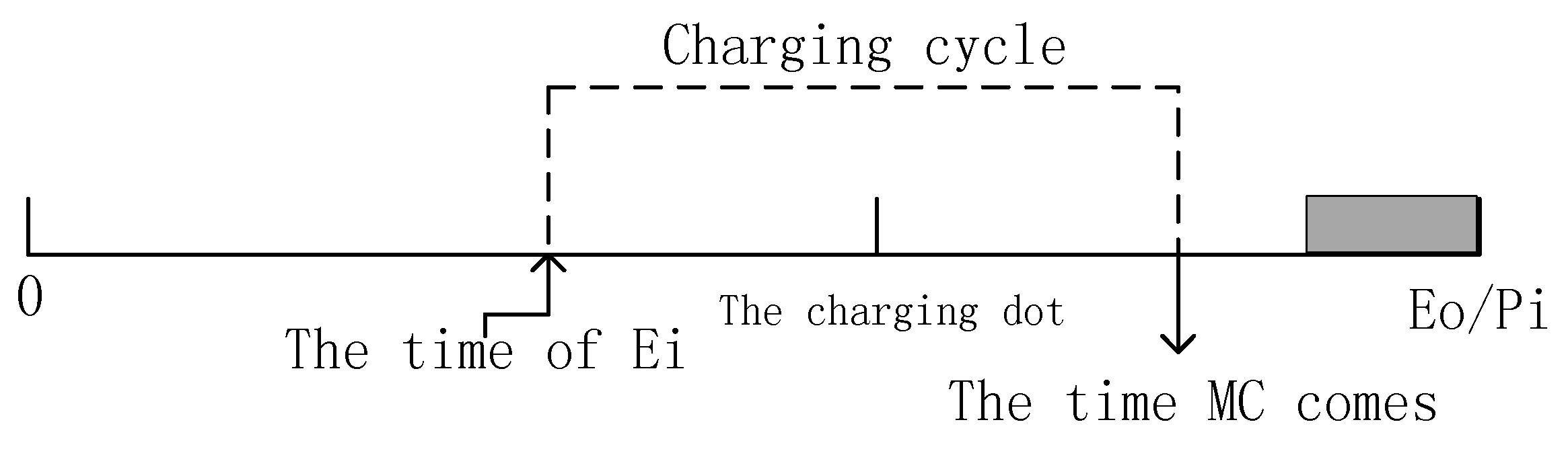
3.1. System Model

Some useful symbols are defined in

Table 1. Symbol and definitions.

Symbol	Definition
$S_i$	Sensor node $i$
$C_j$	Cluster $j$
$E_o$	Initial energy of each sensor node
$e_i^j$	Residual energy of sensor node $S_i$ in cluster $C_j$ when reporting to the sink
$L$	The length of the region
$\theta$	Charging threshold
$V_c$	The traveling velocity of MC
$d$	The valid and farthest charging distance
${\tau }_j$	The serving time of cluster $C_j$
$t_d^j$	The time of data gathering in cluster $C_j$
$t_c^i$	The time of charging for sensor node $S_i$
$t_r^i$	The residual time of sensor node $S_i$
$t_w^j$	The waiting time for MC’s coming to cluster $C_j$
$P_c$	Charging rate of MC
$P_i$	The energy consumption of sensor node $S_i$
$P_d(j)$	The geographic position priority of cluster $C_j$
$P_e(j)$	The residual energy priority of cluster $C_j$
$P(j)$	The combined priority of cluster $C_j$
${\epsilon }_i$	Charging efficiency of sensor node $S_i$
$T$	A charging cycle

.

There are plenty of sensor nodes in the WRSN, we use the set $\{S_1,S_2,\dots ,S_i,\dots ,S_n\}$ to express the sensor nodes, and each sensor node carries the initial energy of $E_o$. Every sensor node can obtain its geographic position and residual energy anytime and anywhere. All sensor nodes are deployed randomly in an $L\times L$ square region, and the sink is located at the center of the region. Several MCs carry enough energy to recharge the sensor nodes with the speed of $V_c$, and in this paper we assumed each MC has enough energy to charge all sensor nodes which need to be served. We defined the valid and farthest charging distance as $d$, and the charging efficiency as ${\epsilon }_i$ of $S_i$. In each cycle, not all the sensor nodes need to be recharged, but all nodes should report data to the sink, and we also proposed the MC as a mobile sink, that is, the MC comes to a cluster to charge several sensor nodes which need to be recharged and collect data of all sensor nodes in this cluster at the same time. In Figure 3, there are several sensor nodes deployed in the region, and in the middle of the region sits the sink. The cycle in Figure 3 represents the cluster, sensor nodes are divided into different clusters, we defined the set of clusters as $\{C_1,C_2,\dots ,C_j,\dots ,C_m\}$, and the MC will stay at the middle of the cluster to charge the sensor nodes and collect data.

When one sensor node $S_i$ is on the verge of exhausting its energy, it will send a charging request to the sink, then the sink arranges a MC to visit the cluster which the sensor node belongs to. The MC starts off from the sink, and follows the route calculated in advance to visit each cluster. After serving all clusters, the MC returns to the sink waiting for the next arrangement. We define ${\tau }_j$ as the time of serving the cluster $C_j$ by the MC, i.e., a MC will stay at cluster $C_j$ for ${\tau }_j$ time to charge sensor nodes and collect data:

$${\tau }_j=\max \{t_d^j,\max \{t_c^1,\dots t_c^i,\dots ,t_c^{n^{\prime }}\}\}$$

(2)

where ${\tau }_j$ is the maximum time for a MC to serve the cluster $C_j$, $t_d^j$ is the time of all sensor nodes in cluster $C_j$ translating their data, $t_c^i$ is the time of the MC charging sensor node $S_i$, and $n^{\prime }$ denotes the number of sensor nodes which need to be charged in a cluster.

The time for the MC to charge the sensor node $S_i$ is $t_c^i$, which can be calculated by Equation (3):

$$t_c^i=\frac{E_o-(e_i^j-t_w^j\times P_i)}{P_c\times {\epsilon }_i}$$

(3)

where $e_i^j(1\le i\le n^{\prime })$ is the residual energy of one sensor node $S_i$ in the cluster $C_j$ when sensor node $S_i$ reports to the sink, $t_w^j$ represents the waiting time of the MC to visit the cluster $C_j$, $P_c$ is the charging speed of the MC, and $P_i$ is the energy consumption of sensor node $S_i$. ${\epsilon }_i$ is the charging efficiency of sensor node $S_i$ according to Equation (1).

Then we can see the waiting time for a MC to visit a cluster $C_j$ is the sum of the serving time of the previous cluster $C_{j-1}$, the waiting time of the previous cluster $C_{j-1}$, and the time of a MC traveling from the previous cluster $C_{j-1}$ to cluster $C_j$. We obtain $t_w^j$ from Equation (4):

$$t_w^j={\tau }_{j-1}+t_w^{j-1}+\frac{dist\{C_j,C_{j-1}\}}{V_c}$$

(4)

Thus, the residual time of a sensor node is calculated by Equation (5):

$$t_r^i=\frac{e_i^j}{P_i}$$

(5)

3.2. Problem Formulation

By the experiment we can know that the energy consumption of communication is closely related to the communication distance. In this paper, the CRMC determined the operating model of the WRSN, which means that the energy consumption of each sensor node can be sharply reduced by a short communication distance. Since every sensor node should be served, data can be totally gathered, finally. However, to ensure the stable operation of the CRMC, there are three problems that need to be solved:

Problem 1:

Does there exist a method of clustering where the MC can charge sensor nodes which are running out of energy and collect data from the all sensor nodes in the same cluster at the same time?

To solve the clustering algorithm, this paper has proposed the HB algorithm to classify sensor nodes.

Problem 2:

How do we design a charging route to ensure the emergency sensor node can be recharged preferential and no sensor nodes die in the whole process?

The charging queue plays the most important role in the whole process, we have considered the comprehensive factors including the residual energy and geographic position to optimize the charging queue.

Problem 3:

One MC cannot satisfy the large WRSN, and sensor nodes could die when the MC comes to visit the cluster in the process. How do we calculate the number of MCs to ensure no sensor nodes run out of energy in each charging cycle?

Too long a charging queue is more likely not to be served by one MC, so we have employed a method to partition the charging queue to calculate the number of MCs by the DMC algorithm.

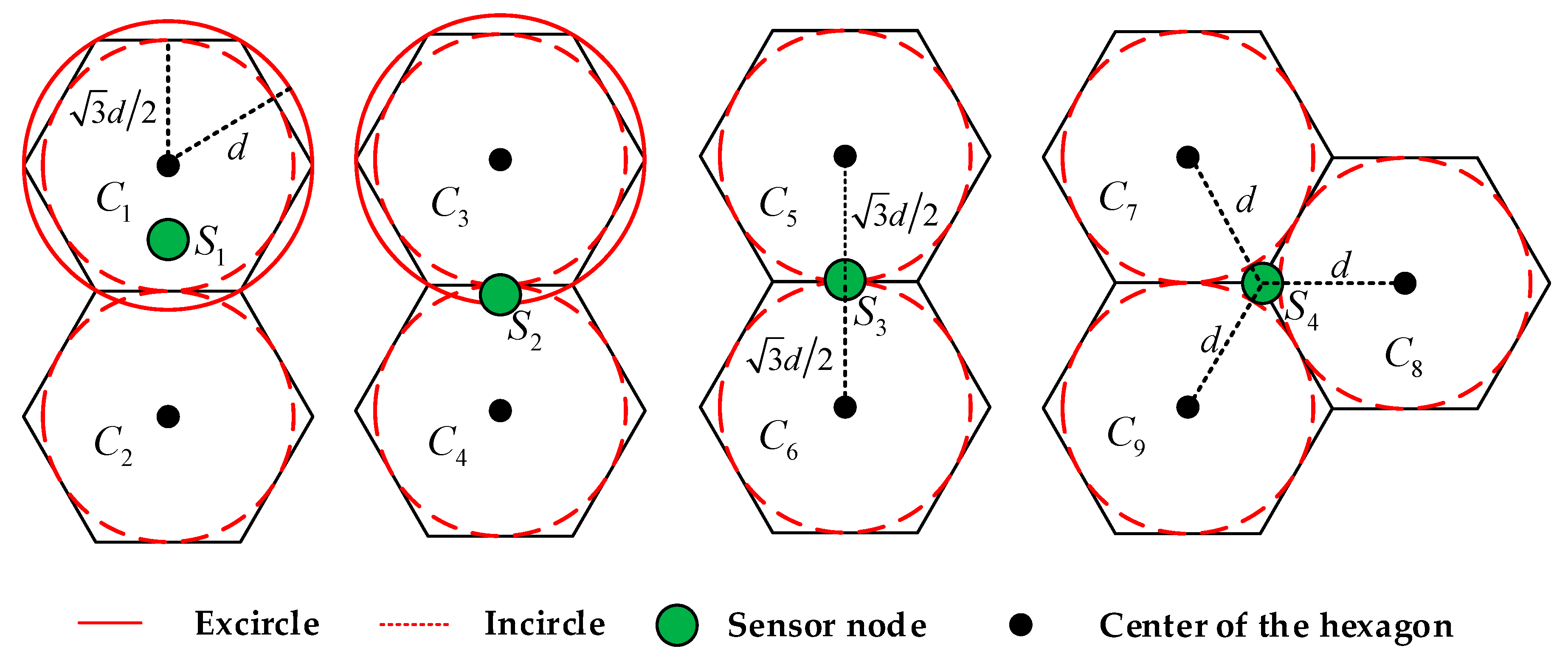
3.3. The Hexagon-Based Algorithm

For problem 1, sensor nodes are divided into several clusters, all sensor nodes in the same cluster need to report data to the MC, but not all sensor nodes need to be recharged. We propose an algorithm based on this work mode, the square region is separated into several hexagonal areas, and each hexagonal area is a cluster, the length of the side is equal to the charging distance $d$, thus, the MC will stand at the middle of the hexagon area. All sensor nodes in the hexagon area are within the charging range $d$, when the MC visits the cluster, sensor nodes which need to be charged can be recharged and all the data can be transported to the MC.

Figure 4 shows the HB algorithm working in a region, several sensor nodes are divided into different hexagonal areas, when the distance between sensor node and the center of the hexagonal area is less than $\sqrt{3}d/2$, i.e., the sensor node is within the limits of the incircle of the hexagon, the sensor node can only belong to one cluster certainly or belong to two possible clusters, also, some sensor nodes sit on the edge of two hexagons or at the point of the three hexagons. In this paper, we propose a method of labelling to distinguish which cluster the sensor node belongs to. This method is illustrated by Figure 5.

We can know that there are four possible positions of the sensor nodes in the WRSN. To distinguish the sensor nodes precisely and fast, we have considered a method of labelling which is shown in Figure 5. We defined x1 to be the condition that the sensor node is in the incircle of the hexagon, in other words, the distance between the sensor node and the center of one hexagon meet the condition: $0\le dist\{S_i,C_j\}<\sqrt{3}d/2$. When the sensor node is within the range of the incircle of the cluster $C_4$ and the excircle of cluster $C_3$ from Figure 5, the distance between sensor node and cluster $C_3$ follows: $\sqrt{3}d/2<dist\{S_2,C_3\}<d$, we use x3 to label the sensor node when the sensor node is in a annulus; similarly, when $dist\{S_3,C_5\}=\sqrt{3}d/2$, there are two hexagons meeting the condition, we use x1 and x2 to label the sensor node of possible clusters; and, lastly, when $dist\{S_4,C_7\}=d$ in Figure 5c, there are three possible clusters and we label the sensor node with x1, x2, and x3 separately, the number of labelling is the serial number of each cluster.

The

Table 2. Labelling of the sensor nodes.

Sensor Node	x1	x2	x3
$S_1$	1	0	0
$S_2$	4	0	3
$S_3$	5	6	0
$S_4$	7	8	9

reflects the different consequences of the labelling of the sensor nodes. For sensor node $S_1$, $0\le dist\{S_1,C_1\}<\sqrt{3}d/2$, so x1 of the $S_1$ is assigned a value of 1, and other labelling parameters are 0. For $S_2$, sensor node is labelled twice, one labelling is when $0\le dist\{S_2,C_4\}<\sqrt{3}d/2$, so the x1 of $S_2$ is bounded of the value of 4, another is when $\sqrt{3}d/2<dist\{S_2,C_3\}<d$, we label the x3 of $S_2$ as 3 and, obviously, $S_2$ is closer to the center point of the hexagon which $S_2$ is in the range of the incircle of cluster $C_4$. We just assign the x3 of $S_2$ with the value of 0, and the sensor node $S_3$ can be confirmed to belong to cluster $C_4$. For $S_3$, the x1 and x2 are labelled with values of 5 and 6 at the same time, that is, the $S_3$ is on the edge of cluster $C_5$ and cluster $C_6$. Then we consider the distance between the cluster and the sink, we choose the closest one to be the appropriate cluster. If the distance is equal, we randomly select from cluster $C_5$ and cluster $C_6$. $S_4$ is at the intersection point of the cluster $C_7$, $C_8$, and $C_9$, and we similarly consider the distance to the sink, and choose the optimal cluster, like $S_3$.

Algorithm 1: Hexagon-Based Algorithm (HB)

1: Initialization: sensor nodes $S_i$ and clusters $C_j$

2: for All $S_i\in S(0<i\le n)$ do

3:  if $0\le dist(S_i,C_j)<\frac{\sqrt{3}}{2}d$ then

4:    Bound the $S_i.x1$ to the value of $j$

5:  else if $dist(S_i,C_j)=\frac{\sqrt{3}}{2}d$ then

6:   Bound the $S_i.x1$ and $S_i.x3$ to the two values of $j$

7:  else if $\frac{\sqrt{3}}{2}d<dist(S_i,C_j)<d$ then

8:   Bound the $S_i.x2$ to the value of $j$

9:  else if $dist(S_i,C_j)=d$ then

10:   Bound the $S_i.x1$ and $S_i.x2$ and $S_i.x3$ to the three values of $j$

11:  end if

12: end for

13: for All $S_i\in S$ do

14:  if $S_i.x1>0$ and $S_i.x3>0$ and $S_i.x2=0$ then

15:   $S_i.x3=0$

16:  else if $S_i.x1>0$ and $S_i.x2>0$ and $S_i.x3=0$ then

17:   Select the cluster which is the closest to the sink, if the distance is equal, choose randomly from the two clusters, bound $S_i.x1$ to the value of $j$ and $S_i.x2$ to the value of 0

18:  else if $S_i.x1>0$ and $S_i.x2>0$ and $S_i.x3>0$ then

19:   Select the cluster which is the closest to the sink, if the distance is equal, choose randomly from the two or three clusters, bound $S_i.x1$ to the value of $j$ and $S_i.x2$, $S_i.x3$ to the value of 0

20:  end if 21: end for

According to Algorithm 1, each sensor node can belong to the optimal cluster, the information is labelled in x1 of each sensor node.

Theorem 1.

The time complexity of the HB algorithm is bounded in$O(n\times m)$, where the$n$and$m$donate the number of the sensor nodes and clusters.

Proof. 

Since $n$ sensor nodes are considered, each sensor node needs to calculate the distance to each cluster, the time complexity of once whole traversal is $O(n\times m)$. Then the time complexity of labelling is $O(n)$, according to the definition of time complexity, and $O(n\times m+n)$ is simplified as $O(n\times m)$. This completes the proof. □

3.4. The Residual Energy and Geographic Position Algorithm

In the WRSN, the residual energy and the geographic position of the sensor nodes should be both considered, in this paper, we have proposed the combination of energy priority and position priority. We use the HB algorithm to distinguish the sensor nodes into different clusters, so which cluster is visited preferentially is of great importance.

We consider the residual energy as the sum of all sensor nodes which need to be recharged in a cluster, it means in a cluster, not all sensor nodes require to be recharged, we only calculate the residual energy of segmental sensor nodes, and the charging efficiency is as a result higher than charging for all sensor nodes. Then the residual energy priority can be provided as:

$$P_e(j)=\frac{{\displaystyle \sum _{n^{\prime }}{e}_i^j}}{n^{\prime }\times E_o}$$

(6)

where the $n^{\prime }$ means the number of sensor nodes which need to be recharged in the cluster $C_j$, $e_i^j$ represents the residual energy of sensor $S_i$ in the cluster $C_j$, obviously the $P_e(j)$ is always lower than 1, and when the $P_e(j)$ is going to 0, the priority of the cluster is larger.

Then we consider the geographic position priority. The first cluster should be the most emergency priority, the residual energy priority of each cluster can be calculated by Equation (6). Then all clusters which need be served should be traversed to calculate the distance to the sink. Combining the residual energy priority $P_e(j)$, the first cluster is founded. As the first cluster is confirmed, the same method is used to find next the most emergency priority cluster. We define the $P_d(j)$ as the geographic position priority:

$$P_d(j)=\frac{dist\{C_j,C_{j^{\prime }}\}}{\sqrt{2}L}$$

(7)

where $dist\{C_j,C_{j^{\prime }}\}$ means the distance between the cluster $C_j$ and the previous cluster $C_{j^{\prime }}$, due to the length of side of the square region is $L$, the longest distance about a MC begins from one cluster to another cluster in the region is $\sqrt{2}L$. Thus, the $P_d(j)$ is also always lower than 1. Similarly, the geographic position priority of a cluster is larger when the $P_d(j)$ is smaller.

Lastly, we combine the residual energy priority and the geographic position priority to obtain the final priority of the cluster:

$$P(j)=\frac{1}{\alpha \times P_e(j)+\beta \times P_d(j)}$$

(8)

We use $\alpha$ and $\beta$ to modify the ratio of the $P_e(j)$ and the $P_d(j)$, and $\alpha$,$\beta$ follows the limits that $\alpha +\beta =1$. When $\alpha$ is equal of 0, the priority of the cluster can be the same as NJNP, and when $\beta$ is equal of 0, the priority of the cluster is the same as EDF. $P(j)$ reflects the priority of a cluster, it determines which cluster is served preferentially. As the $P(j)$ is larger, the priority is higher.

When all sensor nodes which need to be recharged have reported the charging request to the sink, the sink arranges a MC to visit each cluster follows the charging queue. We use the priority to structure the charging queue, because the MC starts from the sink, we consider the head of the queue as the sink, and the remaining elements are all clusters which need to be visited. This means when MC starts from the sink, the forward clusters in the queue can be visited preferentially.

Algorithm 2: Residual Energy and Geographic Position Algorithm (REGP)

Input: The empty sequence of $Q$, sensor nodes $S_i$ and clusters $C_j$

Output: The optimized charging sequence $Q$

1: Let Sink be the head $\in Q$

2: for All $S_i\in S(0<i\le n)$ do

3:  if Energy of $S_i<\theta$ then

4:   $C_j.type=1$, where $j=S_i.x1$

5:  end if

6: end for

7: while Exiting $C_j.type=1$ do

8:  for All $C_j\in C(0<j\le m)$ do

9:   if $C_j.type=1$ then

10:    Calculate the $P(j)$ and find the largest $P(j)$ of $C_j$

11:    $Q\leftarrow Q\cup \left\{C_j\right\}$

12:    $C_j.type=0$

13:   end if

14:  end for

15: end while

16: return $Q$

In Algorithm 2, the sink is joined in queue $Q$ beforehand. When the network begins, all clusters which contain low-energy sensor nodes can be traversed, these clusters are signed as the type of ‘1’. When exiting clusters which need to be served, the first cluster can be found by the largest priority from all clusters. Once the cluster is chosen to be joined into queue $Q$, the type of this cluster transforms into ‘0’. This implies in next traversal, this cluster will not be considered. When all clusters join in queue $Q$, queue $Q$ is accomplished. Ultimately, queue $Q$ contains the sink and all clusters which need to be visited, a MC can follow the queue to serve all clusters need to be visited. When all sensor nodes in queue $Q$ are recharged, one cycle is ended, the other sensor nodes proceed with their work and can be recharged in the next cycle or later.

Theorem 2.

The time complexity of the REGP is bounded in$O(n+m)$.

Proof. 

The worst situation is all sensor nodes need to be recharged and all clusters need to be checked, so the time complexity of traversal is $O(n)$ and the time complexity of checking clusters is $O(m)$, the last time complexity is, therefore, $O(n+m)$.□

3.5. The Dynamic Mobile Charger Algorithm

With the number of sensor nodes increasing, one MC cannot satisfy the whole WRSN. To make sure all sensor nodes are alive throughout the whole process, we need to calculate the least number of MCs to serve the cluster. In this paper, we have raised an algorithm to partition sequence $Q$, the most important constraint is Equation (9), which shows the residual time of one cluster must be larger than the waiting time, so we partition the sequence $Q$ by Equation (9):

$$\min \{t_r^1,\dots t_r^i,\dots ,t_r^{n^{\prime }}\}>t_w^j$$

(9)

$\min \{t_r^1,\dots t_r^i,\dots ,t_r^{n^{\prime }}\}$ determines the sensor node with the least lifetime in cluster $C_j$, if the least survival time of cluster $C_j$ is less than the waiting time $t_w^j$, the sensor node in cluster $C_j$ could die without recharging in time.

However, only with the constraint from Equation (9) is there still a risk of running out of energy. From Figure 6, the horizontal axis means the lifetime of a sensor node, and the sensor node could die when it does not participate in the first charging cycle. During one charging cycle if there is a sensor node that meets the charging threshold, it needs to be charged, but the charger cannot respond to its request. Until the next charging cycle begins, the sensor node could die. Or it could die even though this sensor becomes the first served object joining in the next charging queue, it cannot wait for the MC’s arrival.

$$E_i-T\times P_i>\frac{L}{\sqrt{2}}\times P_i$$

(10)

In Equation (10), the right of the inequation is the longest time of the MC travelling from the sink to the first cluster. When the time of the charging cycle is less than the limit, the sensor node can surely pull through a charging cycle without dying. To ensure all sensor nodes can survive, $E_i$ tends to the charging threshold $\theta$, and the consumption $P_i$ also tends toward the largest value, then the charging cycle $T$ of a MC is limited by Equation (11):

$$T<\frac{\theta }{P_{i\max }}-\frac{L}{\sqrt{2}{V}_c}$$

(11)

Algorithm 3: Dynamic Mobile Charger Algorithm (DMC)

Input: The sequence of $Q$, count number $t$ and the length of $Q$

Output: The number of MCs $k$

1: $t=2$

2: $k=1$

3: Let $l$ as the length of $Q$

4: for All $Q(t)\in Q(1<t\le l)$ do

5:  Calculate the waiting time $t_w^j$

6: end for

7: while $l>1$ do

8:  if The residual time of cluster $Q(t)>t_w^j$ and $T<\frac{\theta }{P_{i\max }}-\frac{L}{\sqrt{2}{V}_c}$ then

9:   $t=t+1$

10:  else

11:   Remove the elements from 2 to $t-1$ and update the $Q$

12:   $k=k+1$

13:   $t=2$

14:   Update the $l$

15:   for All $Q(t)\in Q(1<t\le l)$ do

16:    Calculate the waiting time $t_w^j$

17:   end for

18:  end if

19:  if $l=t-1$ then

20:   $l=0$

21:  end if

22: end while

23: return $k$

The waiting time can be calculated by two adjacent elements in sequence $Q$. For example, since the first element of sequence $Q$ is the sink, then the second element is the first cluster which the MC should visit, and the waiting time is calculated by the distance between the sink and the cluster. Next is the third element, the waiting time is the sum of the waiting time of the first cluster, the serving time of the first cluster, and the time of the MC travels from the first cluster to the second cluster. This is defined in Equation (4). We partition sequence $Q$ once a MC cannot visit the cluster in sequence $Q$ in a timely manner, then we can obtain a charging route for a MC. At the same time we remove these clusters from sequence $Q$, and update $Q$ to repartition the sequence. When all clusters are removed from $Q$ the least number of MCs can be calculated. The serving time of a MC is calculated as follows:

$$T=t_w^j+{\tau }_j+\frac{dist\{C_j,\mathrm{Sin}k\}}{V_c}$$

(12)

A serving time of a MC can be represented by Equation (12), it is the sum of the waiting time of the last cluster in a MC’s charging queue and the serving time by MC, ultimately, the MC returns to the sink.

Theorem 3.

The time complexity is bounded in$O(l^2)$, where$l$donates the length of the sequence$Q$.

Proof. 

Since the head of sequence $Q$ is the sink and the worst situation is all clusters in sequence $Q$ need a MC to serve them, the number of MCs is $l-1$. At the same time, since each cluster needs to calculate the waiting time, the final time complexity is $O({(l-1)}^2)$. According to the definition of time complexity, $O({(l-1)}^2)=O(l^2-2l+1)$ is simplified as $O(l^2)$.□

4. Simulations

In this section, we evaluate the performance of the algorithms by simulation. We set the number of the sensor nodes $n$ as 100, $L$ as 100 m, and the energy consumption $P_i$ of each sensor node is randomly in the range [0.0002, 0.001]. We use the NJNP algorithm and EDF algorithm to compare our algorithms, and we also use the DMC algorithm to calculate the number of MCs in each algorithm.

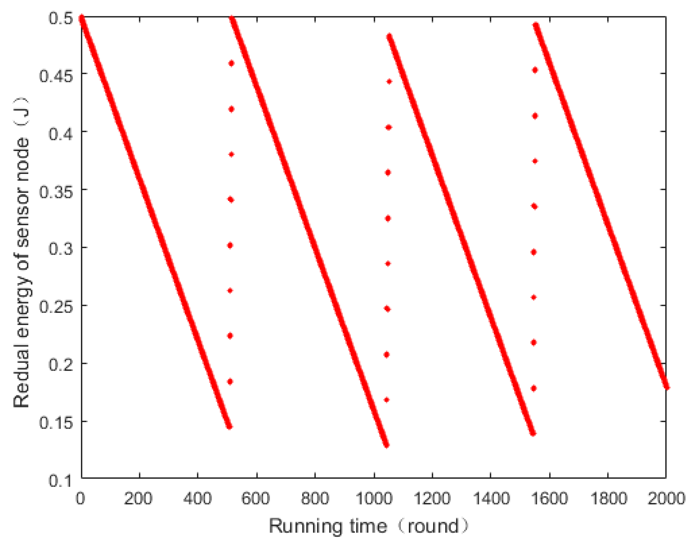
4.1. The Energy Change of a Sensor Node

Once an existing a sensor node needs to be charged, it reports to the sink with a charging request. The whole WRSN can run for a long time without any sensor nodes dying. Due to each sensor node needing to be recharged, the energy of the sensor is changed periodically. In Figure 7, the horizontal axis is the running time, and the ordinate is the residual energy of the sensor node. We can see the energy of the sensor node is always higher than 0.1, and the energy induces a periodic sawtooth-like behavior. When the energy of the sensor node is lower than the charging threshold $\theta$, the MC comes to charge the sensor node. As a result, the energy increases gradually. Since the MC cannot always come to the sensor node in time, the lowest energy in each charging cycle is different. At the same time, due to the sensor node always consuming its energy, the maximum energy is also different after each charging cycle.

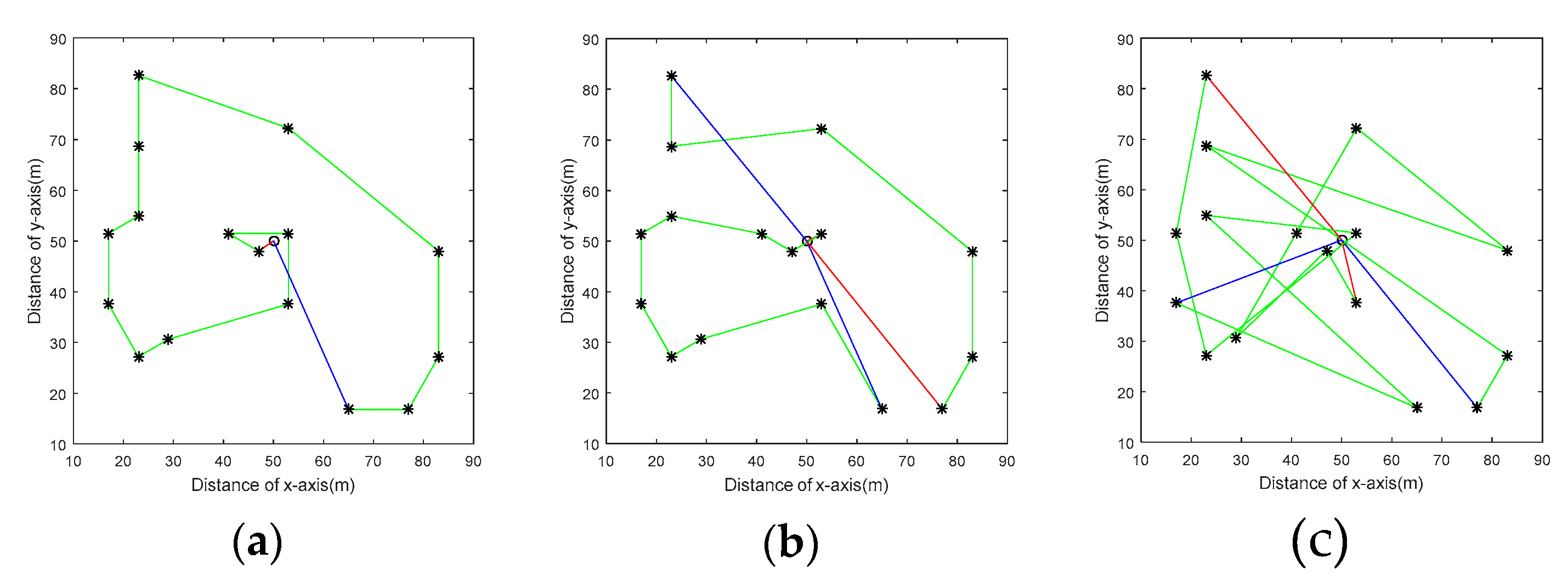
4.2. Path Diagram of One Charging Cycle

The REGP algorithm determines the charging queue of all clusters, and the DMC algorithm calculates the numbers of MCs. In Figure 8, we show the path diagram of REGP compared to NJNP and EDF. With the energy and position considered together, the path of REGP is sharply different to NJNP and EDF. The number of clusters served by the first MC in Figure 5a is 16, but in NJNP the number is 10. The number of MCs in NJNP is 2, however, the number of MCs in our REGP is 1. From Figure 5c, the path diagram of EDF is chaotic, the number of MCs is 2, and due to not considering the position of clusters, a MC can only serve fewer clusters.

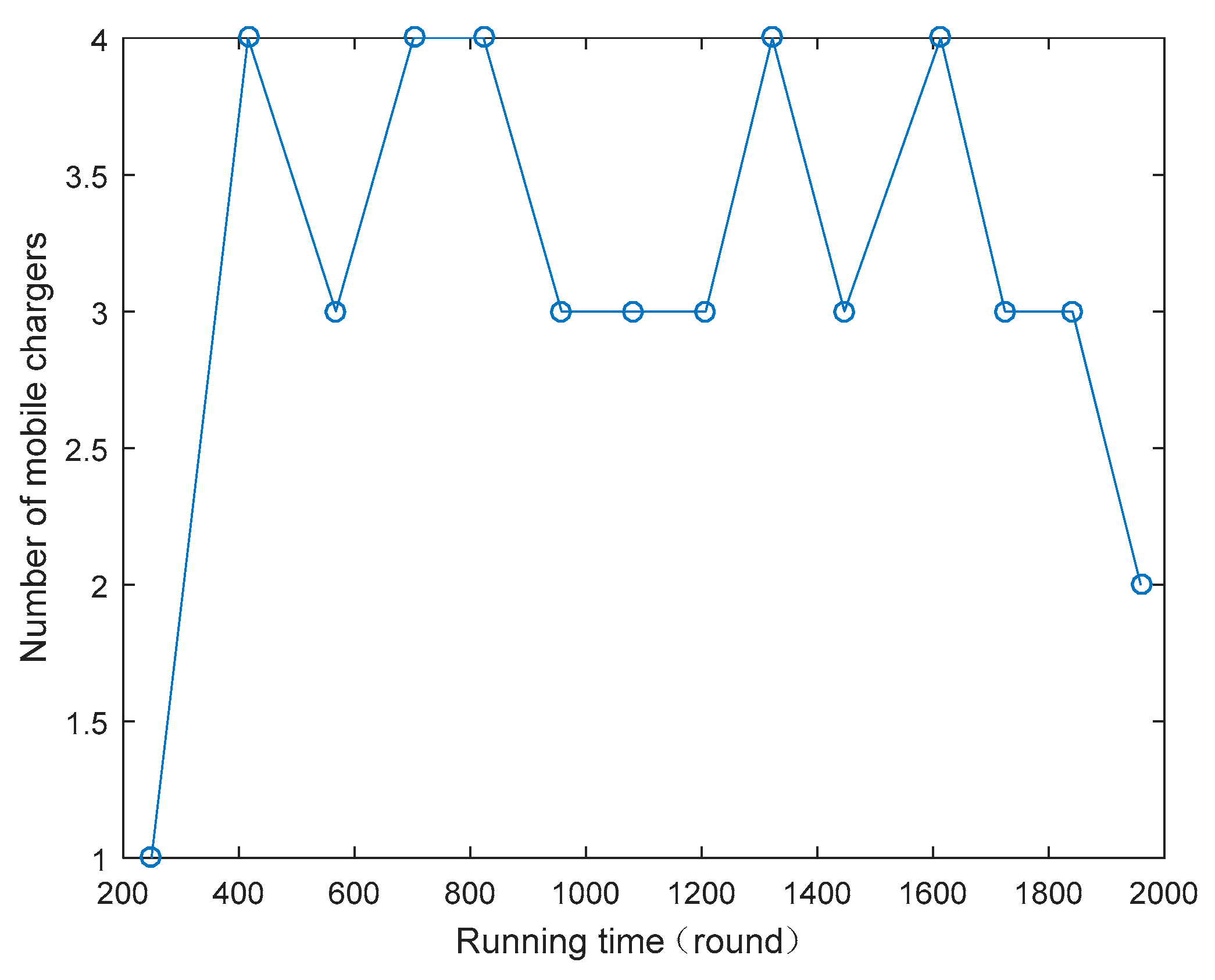
4.3. Number of MCs in Each Charging Cycle

Only one MC cannot serve all sensor nodes in one charging cycle, so several MCs are arranged to ensure no sensor nodes die in the whole process. Since no sensor nodes can die in the WRSN, even if only one sensor node needs to be recharged, the sink should also dispatch a MC to visit the cluster. At the same time, there would be number of sensor nodes that need to be served, so the number of the MCs may also be large. In Figure 9, the maximum number of MCs is 4, and the minimum is 1, and the number of MCs is always changing irregularly. The number of MCs is calculated in advance by the DMC algorithm. When the first charging cycle begins, the DMC algorithm has calculated the number of MCs as 1, and then one MC starts from the sink and serves all clusters needed. The MC returns to the sink after charging, then the next charging cycle begins and the number of MCs increases to 4. The process is always carried out periodically.

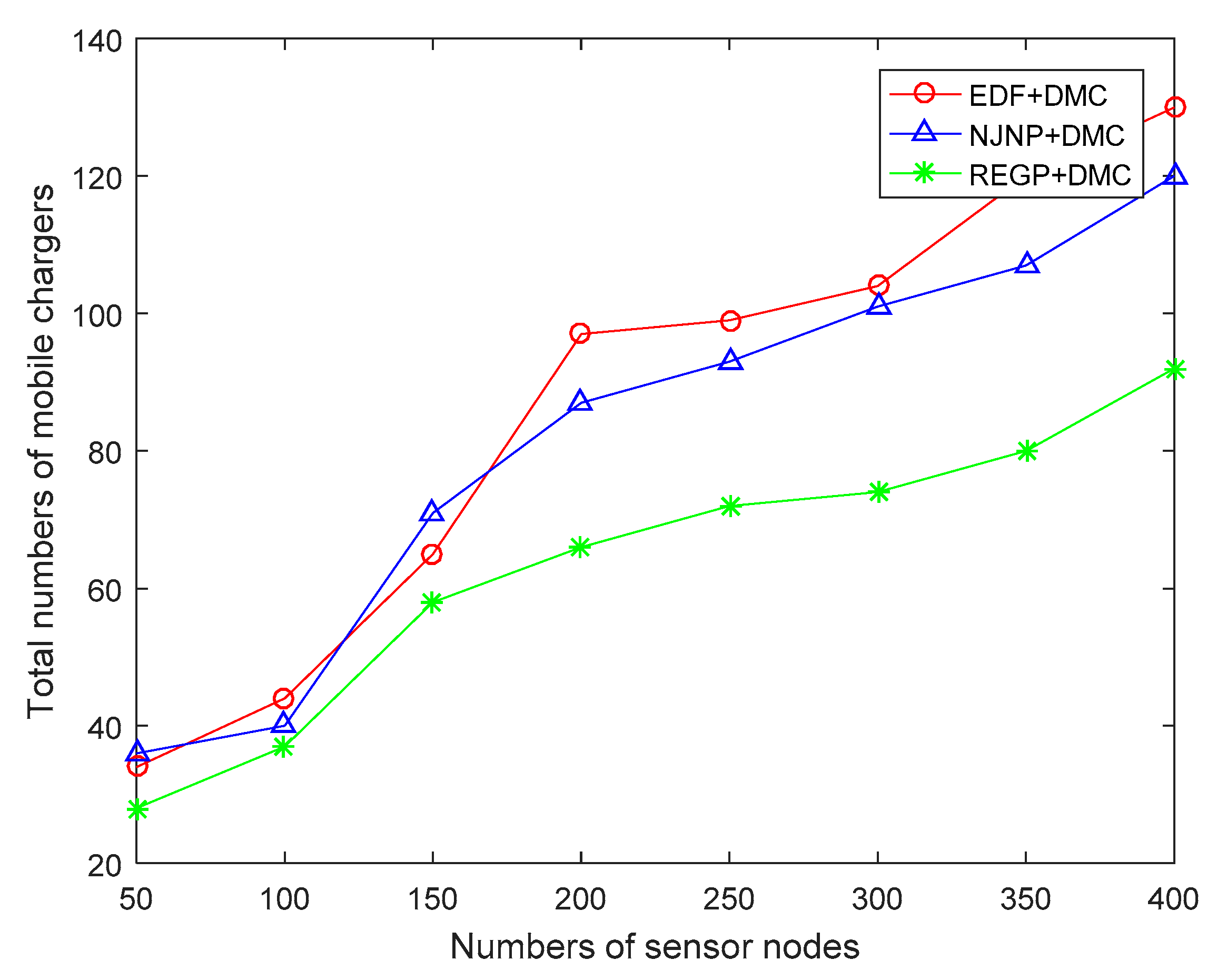
4.4. Total number of MCs in the Whole Process

In this paper, we consider the beginning of the charging as the time when one sensor node meets the charging threshold. That means if only one sensor node needs to be recharged at one time, the sink also arranges a MC to serve the cluster. Thus, the lifecycle of the whole WSRN is largely increased, and the total quantity of MCs in the whole process reflects the charging efficiency of the MCs. The lower number of MCs means a longer charging cycle and a longer serving time of each MC. From Figure 10, the time of the whole process is set as 2000 rounds, with the number of sensor nodes increases, the total quantity of MCs also increases. We can see the EDF and NJNP are always higher than the REGP algorithm, and the REGP algorithm has fewer MCs in each process. With the charging queue not optimized, NJNP may always need more MCs in each charging cycle.

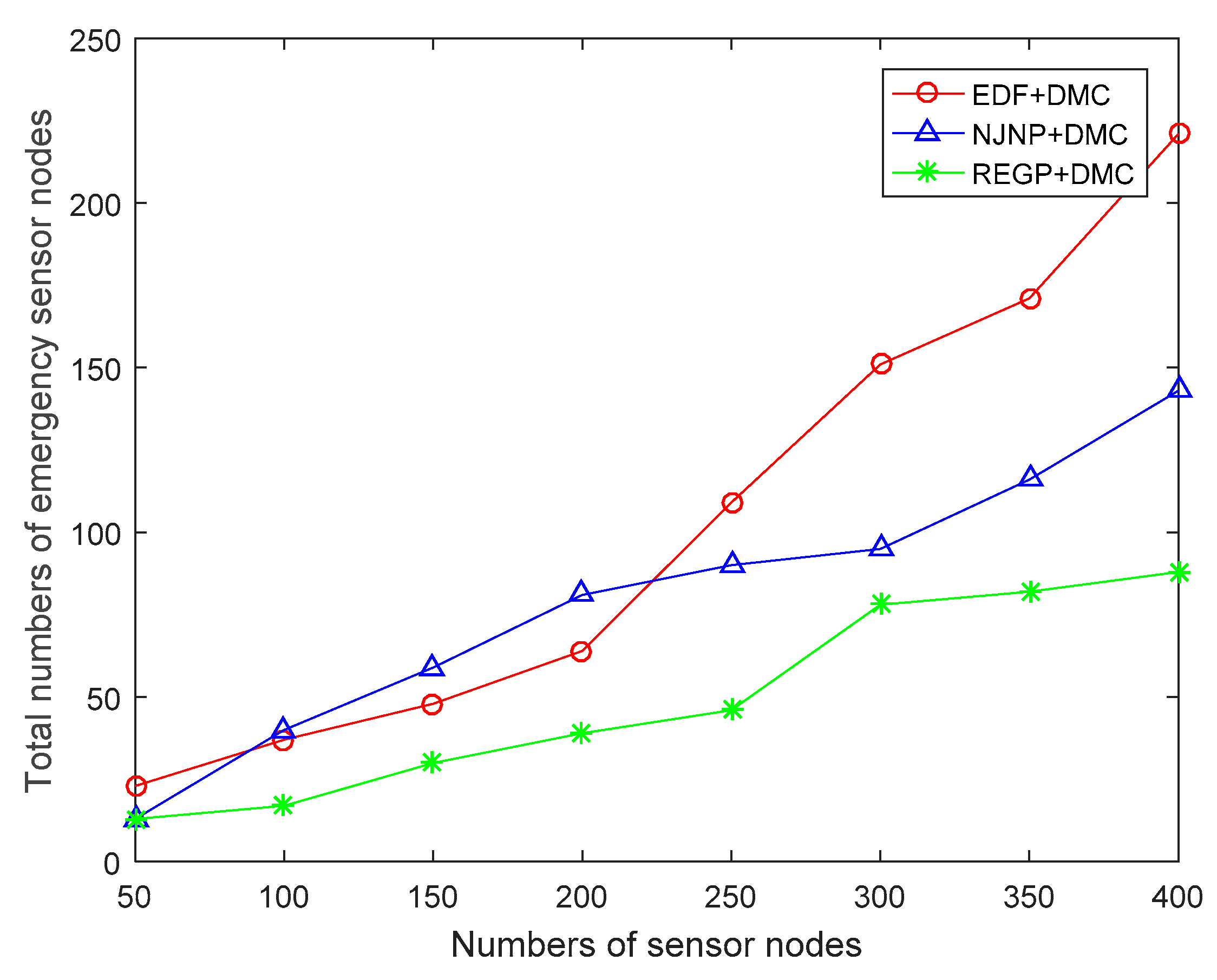
4.5. Total Number of Emergency Sensor Nodes in the Whole Process

Emergency sensor nodes are the sensor nodes which meet one third of the charging threshold, and fewer emergency sensor nodes represent the higher stability of the WSRN. This is owing to the DMC algorithm: with more MCs, more sensor nodes can be recharged in time. From Figure 11, the time of the whole process is also set as 2000 rounds, and the REGP is always lower than EDF and NJNP. With fewer emergency sensor nodes in the whole process, the REGP algorithm performs better than EDF and NJNP, in that the EDF does not consider the position of each sensor, and it could bring about more time of moving of the MC. At the same time, NJNP does not consider the residual energy of each sensor node, causing more emergency sensor nodes not be recharged in time.

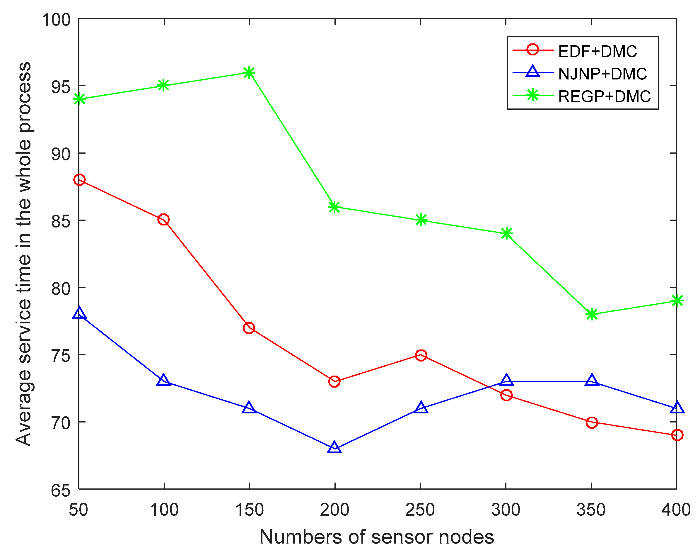
4.6. Average Serving Time of a MC in the Whole Process

In this paper, we consider the serving time with respect to the whole time for a MC to start from the sink and return to the sink. As shown in the Figure 12, with the number of sensor nodes increasing, the average serving time of the whole process decreases, and the decrease is attributed to the increasing number of emergency sensor nodes. To ensure no sensor nodes died, more MCs need to be dispatched to deal with the emergency sensor nodes. From Figure 12, we can also see that the REGP algorithm is always higher than EDF and NJNP. This means that, in the REGP algorithm, the number of emergency sensor nodes is smaller than EDF and NJNP, and higher serving time also represents a higher efficiency of MCs.

5. Conclusions

In order to increase the efficiency of charging and decrease the energy consumption of communication, we use the MC to collect the data when charging. We proposed an effective recharging model, CRCM, in the WRSN. Then, to ensure the MC can collect data and charge at the same time, we propose the HB algorithm to sort all sensor nodes in the region. When the MC comes to the middle of each cluster, all sensor nodes in the cluster can be charged and data can be collected at the same time. Due to the very close communication distance, the energy consumption of communication can be decreased greatly. Then we proposed the REGP algorithm to determine which cluster is visited first. As the priority queue has been established, the DMC algorithm is established to partition the queue to calculate the number of MCs. Finally, we compared the REGP algorithm with EDF and NJNP, the results of the simulation have proved that the REGP algorithm is better than EDF and NJNP algorithm. In the future, we will consider the optimization of the number of MCs in each charging cycle to reduce the average number of MCs.

References

1. Yick, J.; Mukherjee, B.; Ghosal, D. Wireless sensor network survey. Comput. Netw. 2008, 52, 2292–2330. [Google Scholar] [CrossRef]
2. Pottie, G.J.; Kaiser, W.J. Wireless integrated network sensors. Commun. ACM 2004, 43, 51–58. [Google Scholar] [CrossRef]
3. Kansal, A.; Hsu, J.; Zahedi, S.; Srivastava, M.B. Power management in energy harvesting sensor networks. ACM Trans. Embed. Comput. Syst. 2007, 6, 32. [Google Scholar] [CrossRef] [Green Version]
4. Gerla, M.; Tsai, J.T.C. Multicluster, mobile, multimedia radio network. Wirel. Netw. 1995, 1, 255–265. [Google Scholar] [CrossRef]
5. Noh, D.K.; Kang, K. A Practical Flow Control Scheme Considering Optimal Energy Allocation in Solar-Powered WSNs. In Proceedings of the 2009 Proceedings of 18th International Conference on Computer Communications and Networks, San Francisco, CA, USA, 3–6 August 2009; pp. 1–6. [Google Scholar]
6. Li, Y.; Fu, L.; Chen, M.; Chi, K.; Zhu, Y.H. RF-Based Charger Placement for Duty Cycle Guarantee in Battery-Free Sensor Networks. IEEE Commun. Lett. 2015, 19, 1802–1805. [Google Scholar] [CrossRef]
7. Erol-Kantarci, M.; Mouftah, H.T. Challenges of wireless power transfer for prolonging User Equipment (UE) lifetime in wireless networks. In Proceedings of the 2014 IEEE 25th Annual International Symposium on Personal, Indoor, and Mobile Radio Communication (PIMRC), Washington, DC, USA, 2–5 September 2014; pp. 2140–2144. [Google Scholar]
8. Tsiropoulou, E.E.; Mitsis, G.; Papavassiliou, S. Interest-aware Energy Collection & Resource Management in Machine to Machine Communications. Ad Hoc Netw. 2018, 68, 48–57. [Google Scholar]
9. Xie, L.; Shi, Y.; Hou, Y.T.; Lou, A. Wireless power transfer and applications to sensor networks. IEEE Wirel. Commun. 2013, 20, 140–145. [Google Scholar]
10. Shi, Y.; Xie, L.; Hou, Y.T.; Sherali, H.D. On renewable sensor networks with wireless energy transfer. In Proceedings of the 2011 Proceedings IEEE INFOCOM, Shanghai, China, 10–15 April 2011; pp. 1350–1358. [Google Scholar]
11. Tong, B.; Li, Z.; Wang, G.; Zhang, W. How Wireless Power Charging Technology Affects Sensor Network Deployment and Routing. In Proceedings of the 2010 IEEE 30th International Conference on Distributed Computing Systems, Genova, Italy, 21–25 June 2010; pp. 438–447. [Google Scholar]
12. Tsiropoulou, E.E.; Paruchuri, S.T.; Baras, J.S. Interest, Energy and Physical-Aware Coalition Formation and Resource Allocation in Smart IoT Applications. In Proceedings of the 2017 51st Annual Conference on Information Sciences and Systems (CISS), Baltimore, MD, USA, 22–24 March 2017; pp. 1–6. [Google Scholar]
13. He, S.; Chen, J.; Jiang, F.; Yau, D.K.; Xing, G.; Sun, Y. Energy Provisioning in Wireless Rechargeable Sensor Networks. IEEE Trans. Mob. Comput. 2013, 12, 1931–1942. [Google Scholar] [CrossRef] [Green Version]
14. Fu, L.; Cheng, P.; Gu, Y.; Chen, J.; He, T. Optimal Charging in Wireless Rechargeable Sensor Networks. IEEE Trans. Veh. Technol. 2016, 65, 278–291. [Google Scholar] [CrossRef]
15. He, L.; Kong, L.; Gu, Y.; Pan, J.; Zhu, T. Evaluating the On-Demand Mobile Charging in Wireless Sensor Networks. IEEE Trans. Mob. Comput. 2015, 14, 1861–1875. [Google Scholar] [CrossRef]
16. Liang, W.; Xu, W.; Ren, X.; Jia, X.; Lin, X. Maintaining Large-Scale Rechargeable Sensor Networks Perpetually via Multiple Mobile Charging Vehicles. ACM Trans. Sens. Netw. 2016, 12, 14. [Google Scholar] [CrossRef]
17. Dai, H.; Wu, X.; Chen, G.; Xu, L.; Lin, S. Minimizing the number of mobile chargers for large-scale wireless rechargeable sensor networks. Comput. Commun. 2014, 46, 54–65. [Google Scholar] [CrossRef]
18. Kar, K.; Krishnamurthy, A.; Jaggi, N. Dynamic node activation in networks of rechargeable sensors. In Proceedings of the IEEE 24th Annual Joint Conference of the IEEE Computer and Communications Societies, Miami, FL, USA, 13–17 March 2006; pp. 15–26. [Google Scholar]
19. Lin, C.R.; Gerla, M. Adaptive clustering for mobile wireless networks. IEEE J. Sel. Areas Commun. 1997, 15, 1265–1275. [Google Scholar] [CrossRef] [Green Version]
20. He, L.; Gu, Y.; Pan, J.; Zhu, T. On-demand Charging in Wireless Sensor Networks: Theories and Applications. In Proceedings of the 2013 IEEE 10th International Conference on Mobile Ad-Hoc and Sensor Systems, Hangzhou, China, 14–16 Octomber 2013; pp. 28–36. [Google Scholar]
21. Xie, L.; Shi, Y.; Hou, Y.T.; Lou, W.; Sherali, H.D.; Midkiff, S.F. On renewable sensor networks with wireless energy transfer: The multi-node case. In Proceedings of the 2012 9th Annual IEEE Communications Society Conference on Sensor, Mesh and Ad Hoc Communications and Networks (SECON), Seoul, Korea, 18–21 June 2012; pp. 10–18. [Google Scholar]
22. Spuri, M.; Buttazzo, G.C. Efficient aperiodic service under earliest deadline scheduling. In Proceedings of the 1994 Real-Time Systems Symposium, Puerto Rico, USA, 7–9 December 1994; pp. 2–11. [Google Scholar]
23. Karasabun, E.; Korpeoglu, I.; Aykanat, C. Active node determination for correlated data gathering in wireless sensor networks. Comput. Netw. 2013, 57, 1124–1138. [Google Scholar] [CrossRef] [Green Version]
24. Liu, X.; Liu, A.; Li, Z.; Tian, S.; Choi, Y.J.; Sekiya, H.; Li, J. Distributed Cooperative Communication Nodes Control and Optimization Reliability for Resource-Constrained WSNs. Neurocomputing 2017, 270, 122–136. [Google Scholar] [CrossRef]
25. Yang, S.; Yang, X.; McCann, J.A.; Zhang, T.; Liu, G.; Liu, Z. Distributed Networking in Autonomic Solar Powered Wireless Sensor Networks. IEEE J. Sel. Areas Commun. 2014, 31, 750–761. [Google Scholar] [CrossRef]
26. Xie, L.; Shi, Y.; Hou, Y.T.; Lou, W.; Sherali, H.D. On traveling path and related problems for a mobile station in a rechargeable sensor network. In Proceedings of the 14th ACM International Symposium on Mobile Ad Hoc Networking and Computing, Bangalore, India, 29 July–01 August 2013; pp. 109–118. [Google Scholar]
27. Hu, C.; Wang, Y. Optimization of Charging and Data Collection in Wireless Rechargeable Sensor Networks. Int. Conf. Hum. Cent. Comput. 2016, 9567, 138–149. [Google Scholar]
28. Liu, B.H.; Nguyen, N.T.; Pham, V.T.; Lin, Y.X. Novel methods for energy charging and data collection in wireless rechargeable sensor networks. Int. J. Commun. Syst. 2017, 30. [Google Scholar] [CrossRef]
29. Guo, S.; Wang, C.; Yang, Y. Joint Mobile Data Gathering and Energy Provisioning in Wireless Rechargeable Sensor Networks. IEEE Trans. Mob. Comput. 2014, 13, 2836–2852. [Google Scholar] [CrossRef]
30. Guo, S.; Wang, C.; Yang, Y. Mobile data gathering with Wireless Energy Replenishment in rechargeable sensor networks. In Proceedings of the IEEE INFOCOM, Turin, Italy, 14–19 April 2013; pp. 1932–1940. [Google Scholar]
31. Li, J.; Zhao, M.; Yang, Y. OWER-MDG: A novel energy replenishment and data gathering mechanism in wireless rechargeable sensor networks. In Proceedings of the 2012 IEEE Global Communications Conference (GLOBECOM), Anaheim, CA, USA, 3–7 December 2012; pp. 5350–5355. [Google Scholar]
32. Zhou, W.P. Research on Topology Control for Wireless Sensor Networks Based on Cellular Clustering. Master’s Thesis, University Of Anhui, Anhui, China, June 2010. [Google Scholar]
33. Wang, Y.; Vuran, M.C.; Goddard, S. Stochastic Analysis of Energy Consumption in Wireless Sensor Networks. In Proceedings of the 2010 7th Annual IEEE Communications Society Conference on Sensor, Mesh and Ad Hoc Communications and Networks (SECON), Boston, MA, USA, 21–25 June 2010; p. 154. [Google Scholar]
34. TX91501, Powercaster: Pittsburgh, PA, 15238, USA. Available online: Http://www.powercastco.com. (accessed on 30 July 2018).
35. Dai, H.; Liu, Y.; Chen, G.; Wu, X.; He, T. SCAPE: Safe Charging with Adjustable Power. In Proceedings of the 2014 IEEE 34th International Conference on Distributed Computing Systems, Madrid, Spain, 30 June–3 July 2014; pp. 439–448. [Google Scholar]
36. Nittby, H.; Widegren, B.; Krogh, M.; Grafström, G.; Berlin, H.; Rehn, G.; Eberhardt, J.L.; Malmgren, L.; Persson, B.R.; Salford, L.G. Exposure to radiation from global system for mobile communications at 1,800 MHz significantly changes gene expression in rat hippocampus and cortex. Environmentalist 2008, 28, 458–465. [Google Scholar] [CrossRef]
Figure 1. Energy consumption of a sensor node.
Symmetry 10 00319 g001
Figure 2. (a) Experiment of the TX91501. (b) Efficiency of the TX91501 at different distances.
Symmetry 10 00319 g002
Figure 3. System model of the CRCM in the WRSN.
Symmetry 10 00319 g003
Figure 4. Hexagon-based clusters in a region.
Symmetry 10 00319 g004
Figure 5. Four situations of sensor nodes sitting in the region.
Symmetry 10 00319 g005
Figure 6. The situation of not joining in the first charging cycle of the sensor node.
Symmetry 10 00319 g006
Figure 7. Energy change of a sensor node.
Symmetry 10 00319 g007
Figure 8. The comparison of the path diagram by three algorithms. (a) The path diagram of REGP; (b) the path diagram of NJNP; and (c) the path diagram of EDF.
Symmetry 10 00319 g008
Figure 9. Number of MCs in each charging cycle.
Symmetry 10 00319 g009
Figure 10. Total number of MCs in the whole process.
Symmetry 10 00319 g010
Figure 11. Total number of emergency sensor nodes in the whole process.
Symmetry 10 00319 g011
Figure 12. Average serving time of a MC in the whole process.
Symmetry 10 00319 g012