Article

Multi-Granulation Rough Set for Incomplete Interval-Valued Decision Information Systems Based on Multi-Threshold Tolerance Relation

1
School of Sciences, Chongqing University of Technology, Chongqing 400054, China
2
School of Mathematics and Statistics, Southwest University, Chongqing 400715, China
*
Author to whom correspondence should be addressed.
These authors contributed equally to this work.
Symmetry 2018, 10(6), 208; https://doi.org/10.3390/sym10060208
Submission received: 17 May 2018 / Revised: 4 June 2018 / Accepted: 5 June 2018 / Published: 8 June 2018

Abstract

:
A relation is viewed as a granularity from a granular computing perspective. A classic rough set contains only one granularity. A multi-granulation rough set contains multiple granularities, which promotes the applications of classical rough set. Firstly, this paper uses the incomplete interval-valued decision information system (IIVDIS) as research object and constructs two rough set models in the light of single granularity rough set model for applying the rough set theory to real life more widely, which are optimistic multi-granulation rough set (OMGRS) model and pessimistic multi-granulation rough set (PMGRS) model in the IIVDIS. Secondly, we design two algorithms to compute the roughness and the degree of dependence that are two tools for measuring uncertainty of rough set. Finally, several experiments are performed on six UCI data sets to verify the validity of the proposed theorems.

1. Introduction

Pawlak raised rough set theory (RST) [1] in 1982, which has become a relatively complete system after more than thirty years of rapid development. Since the advent of this theory, its strong qualitative analysis [2] makes it a great success in many science and technology fields. As an effective tool for handling ambiguity and uncertainty, the RST has been widely applied in many areas based on its preliminary knowledge. For instance, artificial intelligence, machine learning, data mining, medical diagnosis, algebra [3,4,5,6,7,8,9] and so on. The RST has extended rapidly in recent years and has a lot of fruitful research results [10,11,12,13,14,15,16,17], which is concerned by domestic and foreign scholars and peers.
A subset of universe be often referred to as a concept. The set of these subsets is called knowledge with regard to U. An information system (IS) can represent knowledge and information. Many scholars have studied a variety of rough set problems about information system. Initially, attribute values of the information system are characteristic values or single-values. Later, due to some scholars have different practical needs during their researches, the attribute values are gradually extended to interval numbers, set values, intuitionistic fuzzy numbers, lattice values, etc. and relevant information systems are correspondingly produced [18,19,20,21,22,23]. However, data obtained from real world may exist the phenomena of missing, measurement errors, data noise or other situations. It is inevitable that these reasons will cause the incompleteness of information system. In general, this information system is called an incomplete information system. At first, attribute values studied in the incomplete information system were discrete. Subsequently, the discrete attribute values were extended to continuous values or even other values (such as interval numbers, set values and so on). The classical rough set theory cannot handle problems in incomplete information systems [24,25,26]. Hence many professors pretreated the data, and then used the ideology of the classical RST to solve the problem. These articles [27,28] adopted complete methods to study and deal with the incomplete information system. Nevertheless, these approaches may changed the original data and increased new human uncertainty of information system. Therefore, many scholars provided some relations that were distinct from equivalence relation to avoid changing the original data in the incomplete information system. Zhang [29] studied a method of acquisition rules in incomplete decision tables in the light of similarity relation. The literature [30] calculated the core attribute set based on ameliorative tolerance relationship. Wei [31] optimized the dominance relation and proposed a valued dominance relationship that was negatively/positively concerned in classification analysis. The essay [32] raised α -dominance relationship by using the dominant degree between interval values and gave methods for solving approximate reductions. Gao [33] gave the concept of approximate set based on θ -improved limited tolerance relation. Some researchers [34,35,36,37] took into account preference orders in incomplete ordered information system, and put forward methods to acquire reductions or rules. To study incomplete interval-values information system, Dai [38,39] defined two different similar relations to further explore system uncertainty.
The classification is the foundation of research in RST. From this perspective, a discourse is divided into knowledge granules [40,41,42,43] or concepts. An equivalence relation on the discourse can be considered as a granularity. The partition induced by equivalence relation is treated as a granular space. The classical RST can be seen as a theory that is formed by a single granularity under the equivalence relation. To better apply and promote RST, a new multi-view data analysis method was emerged in recent years, which was data modeling method in multi-granulation rough set (MGRS). Between 1996 and 1997, Zadeh first proposed the concept of granular computing [44]. Qian [45] advanced multi-granulation rough set, which has been researched by many scholars and specialists. However, in practical problems, a discourse is not only divided by one relation, sometimes it will be divided by multiple relations. Faced with this problem, the previously studied single-granularity rough set theory was powerless. It is necessary to consider multiple granularities. Some professors consider fuzzy logic and fuzzy logic inference in [46,47,48]. The literature [49] extended two MGRS models into an incomplete information system. Yang [50] mainly researched several characteristics of MGRS in interval-valued information systems. Xu [51] used the order information system as their investigative object and discussed some measurement methods. Wang [52] introduced the similarity dominance relation for studying MGRS in incomplete ordered decision systems. Yang [53] mainly discussed the relationships among several of multigranulation rough sets in incomplete information system. However, experts and professors have less researches on MGRS in incomplete interval-valued information systems.
To facilitate our discussion, Section 2 mainly introduces some essential notions about RST and incomplete interval-valued decision information system. A single granularity rough set model is established based on the multi-threshold tolerance relation that is defined as the connection degree of Zhao’s [54] set pair analysis. Section 3 establishes two MGRS models (namely, OMRGS model and PMGRS model), and discusses their properties in accordance with the multi-threshold tolerance relation and the viewpoint of multiple granularities. Section 4 explores the uncertainty measure of MGRS in IIVDIS, which are the roughness and the degree of dependence of MGRS in IIVDIS to measure uncertainty of rough set. Section 5 exhibits two algorithms for computing the roughness and the degree of dependence in single granularity rough set and MGRS, respectively. In addition, several UCI data sets are used to verify the correctness of proposed theorems in Section 6. The article ends up with conclusion in Section 7.

2. Preliminaries about RST and IIVDIS

In many cases, we utilize a table to collect data and knowledge. This table regards the universe (that is, objects of discussion) as rows, attributes features represented by objects as columns, which is usually called an information system. For the convenience of the discussion later, this section first gives a few basic definitions [24,38,39].
In general, an information system is denoted as a quadruple I S = ( U , A , V , f ) . When A = C D and C D hold simultaneously, D T = ( U , C D , V , f ) is known as a decision table. It also can be called a decision information system. In here, U is called universe/discourse that represents objects of discussing. Set of characteristics represented by discourse is usually called attribute set A, which contains two parts: the set of condition attributes C and the set of decision attributes D. V a is a subset of V that is the domain of attributes. It can be written as V = a A V a . f : U × A V is a mapping to transform an ordered pair ( x , a ) to a value for each x U , a A . In addition, the mapping is called an information function. Especially, f ( x , d ) ( d D ) is single-valued for every x U .
In mathematics, any subset R of the product of the universe U can be known as a binary relation on U. R is usually referred to as an equivalence relation on U if and only if R satisfies reflexivity, symmetry and transitivity. Pawlak approximation space can be denoted by a binary group U, R. Another mathematical object is the partition on the universe U, which is closely related to the equivalence relation. Specifically, a quotient set is the set of all equivalence classes obtained from the equivalence relation R. It can be easily verify that the quotient set is a partition on U, written down as U / R = { [ x ] R | x U } . Where equivalence class [ x ] R = { y U | x R y } for x U .
If for a A , x U , attribute value ( f ( x , a ) = [ l , l + ] ) is an interval number, then I S is an interval-valued information system, referred to as I I S = ( U , A , V , f ) . Particularly, if l = l + , f ( x , a ) is a real number, so the interval-valued information system is the generalization of classical information system. Where l , l + R , R is the set of real number.
Let f ( x , a ) = [ l , l + ] , if at least one of lower bound l and upper bound l + is an unknown value, thus we will write down as f ( x , a ) = * . In addition, I I I S = ( U , A , V , f ) is an incomplete interval-valued information system. I I D I S = ( U , C D , V , f ) is an incomplete interval-valued decision information system or incomplete interval-valued decision table. In the following discussion, we only discuss the situation where D = { d } .
Definition 1.
Given an incomplete interval-valued information system I I I S = ( U , A , V , f ) , for ∀ a k A , x i , x j U . The attribute values of two objects x i , x j are not *. Let f k ( x i , a ) = μ = [ μ , μ + ] , f k ( x j , a ) = ν = [ ν , ν + ] , then the similarity degree [55] with reference to x i , x j under the attribute a k is
S i j k ( μ , ν ) = | μ ν | | μ ν | .
In the above equation, | · | represents the length of the closed interval. The similarity degree can also be transformed as
S i j k ( μ , ν ) = | μ ν | | μ | + | ν | | μ ν | .
Remark 1.
(1)
The length of the empty set and the single-point set are equal to zero;
(2)
Assume that two attribute values are single-point set. If μ = ν , then S i j k ( μ , ν ) = 1 ; if μ ν , then S i j k ( μ , ν ) = 0 .
(3)
If μ = * or ν = * or μ = * , ν = * , then set the similarity degree with respect to x i , x j equals ▲.
Definition 2.
[54] Let two sets Q, G constitute a set pair H = ( Q , G ) . According to the need of the problem W, we can analyze the characteristics of set pair H, and obtain N characteristics (attributes). For two sets Q, G, which have same values on S attributes, different values on P attributes, and the rest of F = N S P attribute values are ambiguous. S N is called the identical degree of these two sets under problem W. Referred to as the identical degree. P N is called the opposite degree of these two sets under problem W. Referred to as the opposite degree. F N is called the difference degree of these two sets under problem W. Referred to as the difference degree. Then the connection degree with respect to two sets Q, G can be defined as
μ ( Q , G ) = S N + F N · i + P N · j .
Denoted as μ ( Q , G ) = s + f · i + p · j . Where s , f , p [ 0 , 1 ] , s + f + p = 1 . In the calculation, set j = 1 , i [ 1 , 1 ] , i and j also participate in the operation as coefficients. However, the function of i, j are just markings in this paper. i is the marking of the difference degree, j is the marking of the opposite degree.
Given an incomplete interval-valued information system (IIIS), the similarity degree of the two objects can be calculated in the light of the values of Definition 1. There are three possible cases:
(1)
The two attribute values are both not equal to *, and their similarity degree is greater than or equal to a given threshold;
(2)
The two attribute values are both not equal to *, and their similarity degree is less than a given threshold;
(3)
At least one of the two attribute values is equal to *, and their similarity degree is considered to be ▲.
Definition 3.
[56] Given an incomplete interval-valued information system I I I S = ( U , A , V , f ) , B A , x i , x j U . Let S 1 = { b k B | ( S i j k ( μ , ν ) λ ) ν * μ * } is a set of the attributes that the similarity degree of x i , x j under the attribute b k is not less than a similar level λ. P 1 = { b k B | S i j k ( μ , ν ) < λ ν * μ * } is a set of the attributes that the similarity degree of x i , x j under the attribute b k is less than a similar level λ. F 1 = { b k B | S i j k ( μ , ν ) = } is a set of the attributes that the similarity degree of x i , x j under the attribute b k is equal to ▲.
Where | S 1 | | B | shows the tolerance degree of the two objects with regard to B. | P 1 | | B | shows the opposite degree of the two objects with regard to B. | F 1 | | B | shows the difference degree of the two objects with regard to B. Then the relationship of x i , x j is known as
μ 1 ( x i , x j ) = | S 1 | | B | + | F 1 | | B | · i + | P 1 | | B | · j .
μ 1 indicates similar connection degree of the two objects x i , x j . Referred to as μ 1 ( x i , x j ) = s 1 + f 1 · i + p 1 · j . Where s 1 , f 1 , p 1 [ 0 , 1 ] , s 1 + f 1 + p 1 = 1 , the function of i, j are just markings. i is the marking of the difference degree, j is the marking of the opposite degree.
It is unreasonable to put two objects in the same class only if the tolerance degree of the two objects under the attribute subset is equal to 1. In [56], the paper considers the tolerance degree and the opposite degree but is unaware of difference degree. Whether two objects x 1 , x 2 should be classified as the same class, the article [56] defines the tolerance relation based on similarity connection degree to solve this problem. In there, we assume that λ = 0.5 , α = 0.6 , β = 0.2 and there are five attributes, that is B = { a 1 , a 2 , a 3 , a 4 , a 5 } . If attribute values of x 1 , x 2 under the attribute set B are [ 1 , 2 ] , [ 1 , 3 ] , [ 1 , 5 ] , [ , 2 ] , [ , 1 ] and [ 1 , 2 ] , [ 1 , 4 ] , [ 1 , 5 ] , [ 5 , ] , [ 2 , ] , respectively. We can see from the calculation that ( x 1 , x 2 ) B α β ( B α β is the tolerance relation based on similarity connection degree in [56]). However, it is obvious that the attribute values of x 1 , x 2 under attribute a 4 , a 5 are absolutely different. Therefore, in order to better study the information system containing multiple unknown values or missing parts. Based on the above discussion, this article also considers the difference degree apart from the tolerance degree and the opposite degree. The concrete method is: the tolerance degree of the two objects under the attribute subset is greater than or equal to α and the opposite degree of the two objects under the attribute subset is less than or equal to β. Moreover, the difference degree of the two objects under the attribute subset is less than or equal to γ. In summary, the multi-threshold tolerance relation is given below.
Definition 4.
In the incomplete interval-valued decision information system (IIVDIS) I I V D I S = ( U , C { d } , V , f ) , for any B C , x i , x j U . α ( 0.5 , 1 ] , β , γ [ 0 , 0.5 ) . The multi-threshold tolerance relation can be referred as
R B α β γ = { ( x i , x i ) } { ( x i , x j ) | μ 1 ( x i , x j ) = s 1 + f 1 · i + p 1 · j , s 1 α , f 1 γ , p 1 β , s 1 + f 1 + p 1 = 1 }
s 1 , f 1 , p 1 represent, respectively, the tolerance degree, the difference degree and the opposite degree of objects x i , x j with reference to B. α is the threshold of the tolerance degree, β is the threshold of the opposite degree, γ is the threshold of the difference degree.
The multi-threshold tolerance class can be defined as
[ x i ] R B α β γ = { x j U | ( x i , x j ) R B α β γ } .
U / R B α β γ = { [ x 1 ] R B α β γ , [ x 2 ] R B α β γ , , [ x | U | ] R B α β γ } .
In addition, a binary relation under decision attribute d is remembered as R d = { ( x i , x j ) U 2 | f d ( x i ) = f d ( x j ) } . Decision class and quotient set can be alluded to as [ x ] d = { y U | f d ( x ) = f d ( y ) } , U / d = { [ x ] d | x U } = { D 1 , D 2 , , D q } ( D i U , i = 1 , 2 , , q ) , respectively. Obviously, relation R d is an equivalence relation and U / d constitutes a partition on U.
Remark 2.
(1)
It obviously observes that the multi-threshold tolerance relation is reflexive and symmetrical rather than transitive, which is a tolerance relation; J = { [ x i ] R B α β γ } is a cover on U.
(2)
It is reasonable to put two objects in the same class if the tolerance degree of the two objects under the attribute subset is not less than α and the opposite degree, the difference degree of the two objects under the attribute subset is less than or equal to β, γ, respectively.
(3)
If we don’t consider parameter γ and the range of α , β , the multi-threshold tolerance relation is degraded into the tolerance relation in [56]. Therefore, the tolerance relation in [56] can be regarded as a specific situation of multi-threshold tolerance relation.
(4)
When B = { a } , { a } can be replaced by a. The following paper will denote R a α β γ , [ x i ] R a α β γ , U / R a α β γ .
Definition 5.
In the I I V D I S = ( U , C { d } , V , f ) , for each B C , X U . The approximations of X concerning a multi-threshold tolerance relation R B α β γ can be represented by
R B α β γ ̲ ( X ) = { x U | [ x ] R B α β γ X } ; R B α β γ ¯ ( X ) = { x U | [ x ] R B α β γ X } .
R B α β γ ̲ , R B α β γ ¯ are called lower and upper approximation operator of X concerning a multi-threshold tolerance relation R B α β γ .
Moreover, similar to classical rough set, positive region is recorded as P o s R B α β γ ( X ) = R B α β γ ̲ ( X ) , negative region is known as N e g R B α β γ ( X ) = U R B α β γ ¯ ( X ) , what boundary region represents the difference between the lower approximation and upper approximation of X concerning R B α β γ is denoted by B n R B α β γ ( X ) = R B α β γ ¯ ( X ) R B α β γ ̲ ( X ) .
Some relationships between upper and lower approximation are similar to the properties of upper and lower approximation of the classical rough set. Detailed results are as follows.
Theorem 1.
In the I I V D I S = ( U , C { d } , V , f ) , for any B C , X , Y U . There have
(1) R B α β γ ̲ ( X ) X R B α β γ ¯ ( X ) .(Boundedness)
(2) R B α β γ ̲ ( X ) = R B α β γ ¯ ( X ) ; R B α β γ ¯ ( X ) = R B α β γ ̲ ( X ) .(Duality)
(3) R B α β γ ̲ ( ) = R B α β γ ¯ ( ) = ; R B α β γ ̲ ( U ) = R B α β γ ¯ ( U ) = U .(Normality)
(4) R B α β γ ̲ ( X Y ) = R B α β γ ̲ ( X ) R B α β γ ̲ ( Y ) ; R B α β γ ¯ ( X Y ) = R B α β γ ¯ ( X ) R B α β γ ¯ ( Y ) .(Multiplicativity and Additivity)
(5)If X Y holds, then R B α β γ ̲ ( X ) R B α β γ ̲ ( Y ) and R B α β γ ¯ ( X ) R B α β γ ¯ ( Y ) .(Monotonicity)
(6) R B α β γ ̲ ( X Y ) R B α β γ ̲ ( X ) R B α β γ ̲ ( Y ) ; R B α β γ ¯ ( X Y ) R B α β γ ¯ ( X ) R B α β γ ¯ ( Y ) .(Inclusion)
Proof. 
( 1 ) For x R B α β γ ̲ ( X ) , have [ x ] R B α β γ X . If x [ x ] R B α β γ , thus x X hold. So R B α β γ ̲ ( X ) X . For x X . x [ x ] R B α β γ must be hold on account of R B α β γ satisfies reflexivity, so [ x ] R B α β γ X . That is x R B α β γ ¯ ( X ) . Hence X R B α β γ ¯ ( X ) .
From the above, we can prove that R B α β γ ̲ ( X ) X R B α β γ ¯ ( X ) .
( 2 ) For x R B α β γ ̲ ( X ) , according to Definition 5 (Equation (8)), there have [ x ] R B α β γ X [ x ] R B α β γ X = x R B α β γ ¯ ( X ) x R B α β γ ¯ ( X ) .
In summary, R B α β γ ̲ ( X ) = R B α β γ ¯ ( X ) . Obviously, R B α β γ ¯ ( X ) = R B α β γ ̲ ( X ) , therefore, R B α β γ ¯ ( X ) = R B α β γ ̲ ( X ) .
( 3 ) It can be known from ( 1 ) of this theorem that R B α β γ ̲ ( ) , moreover, it is evident that R B α β γ ̲ ( ) , so R B α β γ ̲ ( ) = .
Suppose that R B α β γ ¯ ( ) , then there must be exists x R B α β γ ¯ ( ) s.t. [ x ] R B α β γ , which is a contradiction with [ x ] R B α β γ = . Hence R B α β γ ¯ ( ) = .
From the proof of ( 2 ) of this theorem, we can see R B α β γ ̲ ( U ) = R B α β γ ¯ ( U ) = R B α β γ ¯ ( ) = = U . R B α β γ ¯ ( U ) = R B α β γ ̲ ( U ) = R B α β γ ̲ ( ) = = U .
( 4 ) For x R B α β γ ̲ ( X Y ) , have [ x ] R B α β γ X Y [ x ] R B α β γ X and [ x ] R B α β γ Y x R B α β γ ̲ ( X ) and x R B α β γ ̲ ( Y ) x R B α β γ ̲ ( X ) R B α β γ ̲ ( Y ) .
For x R B α β γ ¯ ( X Y ) , have [ x ] R B α β γ ( X Y ) [ x ] R B α β γ X or [ x ] R B α β γ Y x R B α β γ ¯ ( X ) or x R B α β γ ¯ ( Y ) x R B α β γ ¯ ( X ) R B α β γ ¯ ( Y ) .
( 5 ) Since X Y , so R B α β γ ̲ ( X Y ) = R B α β γ ̲ ( X ) . Under the equation ( 4 ) of this theorem, R B α β γ ̲ ( X Y ) = R B α β γ ̲ ( X ) R B α β γ ̲ ( Y ) . Therefore, R B α β γ ̲ ( X ) = R B α β γ ̲ ( X ) R B α β γ ̲ ( Y ) . In other words, R B α β γ ̲ ( X ) R B α β γ ̲ ( Y ) .
Since X Y , so R B α β γ ¯ ( X Y ) = R B α β γ ¯ ( Y ) . Under the equation ( 4 ) of this theorem, R B α β γ ¯ ( X Y ) = R B α β γ ¯ ( X ) R B α β γ ¯ ( Y ) . Therefore, R B α β γ ¯ ( Y ) = R B α β γ ¯ ( X ) R B α β γ ¯ ( Y ) . In other words, R B α β γ ¯ ( X ) R B α β γ ¯ ( Y ) .
( 6 ) For X X Y , Y X Y . In the light of the equation ( 5 ) of this theorem, we can acquire R B α β γ ̲ ( X ) R B α β γ ̲ ( X Y ) , R B α β γ ̲ ( Y ) R B α β γ ̲ ( X Y ) . So R B α β γ ̲ ( X ) R B α β γ ̲ ( Y ) R B α β γ ̲ ( X Y ) .
For X Y X , Y . According to the equation ( 5 ) of this theorem, we can obtain R B α β γ ¯ ( X Y ) R B α β γ ¯ ( X ) , R B α β γ ¯ ( X Y ) R B α β γ ¯ ( Y ) . So R B α β γ ¯ ( X Y ) R B α β γ ¯ ( X ) R B α β γ ¯ ( Y ) ,
Inspired by the roughness of X with regard to the classical approximation space. Following definition describes the roughness and the degree of dependence of X based on the multi-threshold tolerance relation in single granularity rough set. ☐
Definition 6.
In the I I V D I S = ( U , C { d } , V , f ) , for any B C , X U . Then the roughness of X is
ρ B α β γ ( X ) = 1 | R B α β γ ̲ ( X ) | | R B α β γ ¯ ( X ) | .
Moreover, what the quality of approximation of d is decided by B is referred to as the degree of dependence. It can be denoted as
δ ( B , d ) = 1 | U | · j = 1 q | R B α β γ ̲ ( D j ) | .

3. Two Multi-Granulation Rough Set Models in IIVDIS

The classical rough set studies the single-granularity space when an equivalence relation in the discourse is regarded as a granularity. According to the needs of real life, it is also very significant to research multiple granularities. For every x, a multi-threshold tolerance class induced by the multi-threshold tolerance relation be considered as a granule. In IIVDIS, multiple multi-threshold tolerance relations and multiple granules are obtained in consideration of multiple granularities. There are four situations:
(a)
At least one granule is contained in a given concept;
(b)
All granules have intersection with a given concept;
(c)
All granules can be included in a given concept;
(d)
At least one granule can intersect with a given concept.
We can utilize (a) and (b) to depict lower approximation and upper approximation (approximations for short) of the multi-granulation rough set under optimistic situation. (c) and (d) are treated as main idea for defining approximations of the multi-granulation rough set under pessimistic circumstance. The following will elaborate the OMGRS and PMGRS.

3.1. The Optimistic Multi-Granulation Rough Set in IIVDIS

To more broadly apply RST to the complex IIVDIS of real life, this section studies multiple granularities on the basis of the multi-threshold tolerance relation. For the sake of convenience, the proof of all the following theorems only consider the case with respect to two granularities while the studied granularities are limited.
Definition 7.
In the I I V D I S = ( U , C { d } , V , f ) , B 1 , B 2 , , B t C ( t 2 | C | ), X P ( U ) . The following defines two operators O C i = 1 t B i α β γ ̲ and O C i = 1 t B i α β γ ¯ on P ( U ) :
O C i = 1 t B i α β γ ̲ ( X ) = { x U | i = 1 t [ x ] R B i α β γ X } ; O C i = 1 t B i α β γ ¯ ( X ) = { x U | i = 1 t [ x ] R B i α β γ X } .
where P ( U ) is all subsets of U, , represent the meaning of o r , a n d , respectively. O C i = 1 t B i α β γ ̲ ( X ) and O C i = 1 t B i α β γ ¯ ( X ) are known as lower approximation and upper approximation of X concerning optimistic multi-granulation in the IIVDIS, respectively.
If O C i = 1 t B i α β γ ̲ ( X ) = O C i = 1 t B i α β γ ¯ ( X ) , we call that X is the optimistic exact set in the IIVDIS. If not, X is called the optimistic rough set.
According to prior definition, in the IIVDIS, the boundary region of optimistic rough set is
B n i = 1 t B i O C ( X ) = O C i = 1 t B i O C ¯ ( X ) O C i = 1 t B i α β γ ̲ ( X ) .
The boundary region of optimistic rough set denotes the distinction of both approximations in the IIVDIS. When B n i = 1 t B i O C ( X ) = 0 , then X is the optimistic exact set. Otherwise, X is the optimistic rough set.
Theorem 2.
In the I I V D I S = ( U , C { d } , V , f ) , B 1 , B 2 , , B t C ( t 2 | C | ), X , Y P ( U ) . Then approximations of the optimistic multi-granulation satisfy the following properties:
(1) O C i = 1 t B i α β γ ̲ ( X ) X O C i = 1 t B i α β γ ¯ ( X ) . (Optimistic boundedness)
(2) O C i = 1 t B i α β γ ̲ ( X ) = O C i = 1 t B i α β γ ¯ ( X ) , O C i = 1 t B i α β γ ¯ ( X ) = O C i = 1 t B i α β γ ̲ ( X ) . (Optimistic duality)
(3) O C i = 1 t B i α β γ ̲ ( ) = O C i = 1 t B i α β γ ¯ ( ) = , O C i = 1 t B i α β γ ̲ ( U ) = O C i = 1 t B i α β γ ¯ ( U ) = U . (Optimistic normality)
(4) O C i = 1 t B i α β γ ̲ ( X Y ) O C i = 1 t B i α β γ ̲ ( X ) O C i = 1 t B i α β γ ̲ ( Y ) ,
O C i = 1 t B i α β γ ¯ ( X Y ) O C i = 1 t B i α β γ ¯ ( X ) O C i = 1 t B i α β γ ¯ ( Y ) .
(Optimistic inclusion 1)
(5)If X Y , then O C i = 1 t B i α β γ ̲ ( X ) O C i = 1 t B i α β γ ̲ ( Y ) , O C i = 1 t B i α β γ ¯ ( X ) O C i = 1 t B i α β γ ¯ ( Y ) . (Optimistic monotonicity)
(6) O C i = 1 t B i α β γ ̲ ( X Y ) O C i = 1 t B i α β γ ̲ ( X ) O C i = 1 t B i α β γ ̲ ( Y ) ,
O C i = 1 t B i α β γ ¯ ( X Y ) O C i = 1 t B i α β γ ¯ ( X ) O C i = 1 t B i α β γ ¯ ( Y ) .
(Optimistic inclusion 2)
Proof. 
For convenience of description, here let t = 2 , that is B 1 , B 2 . When B 1 = B 2 , these properties are clearly established. Now prove the case of B 1 B 2 .
(1) For x O C B 1 + B 2 α β γ ̲ ( X ) , there have [ x ] R B 1 α β γ X or [ x ] R B 2 α β γ X . In addition, because multi-threshold tolerance relation satisfies reflexivity, forasmuch x [ x ] R B 1 α β γ and x [ x ] R B 2 α β γ . It can be acquired that x X . Hence, O C B 1 + B 2 α β γ ̲ ( X ) X .
For x X , apparently, x [ x ] R B 1 α β γ and x [ x ] R B 2 α β γ . So [ x ] R B 1 α β γ X and [ x ] R B 2 α β γ X . According to the Definition 7 (Equation (11)), x O C B 1 + B 2 α β γ ¯ ( X ) . Therefore, X O C B 1 + B 2 α β γ ¯ ( X ) .
Therefore, we can prove O C B 1 + B 2 α β γ ̲ ( X ) X O C B 1 + B 2 α β γ ¯ ( X ) .
(2) For x O C B 1 + B 2 α β γ ̲ ( X ) , have
[ x ] R B 1 α β γ X or [ x ] R B 2 α β γ X [ x ] R B 1 α β γ X = or [ x ] R B 2 α β γ X = x O C B 1 + B 2 α β γ ¯ ( X ) x O C B 1 + B 2 α β γ ¯ ( X ) .
In summary, O C B 1 + B 2 α β γ ̲ ( X ) = O C B 1 + B 2 α β γ ¯ ( X ) .
If O C B 1 + B 2 α β γ ̲ ( X ) = O C B 1 + B 2 α β γ ¯ ( X ) , then O C B 1 + B 2 α β γ ¯ ( X ) = O C B 1 + B 2 α β γ ̲ ( X ) . So O C B 1 + B 2 α β γ ¯ ( X ) = O C B 1 + B 2 α β γ ̲ ( X ) .
(3) It can be got from property ( 1 ) of this theorem that O C B 1 + B 2 α β γ ̲ ( ) , moreover, it is clear that O C B 1 + B 2 α β γ ̲ ( ) , so O C B 1 + B 2 α β γ ̲ ( ) = .
Suppose that O C B 1 + B 2 α β γ ¯ ( ) , then there must be exists x O C B 1 + B 2 α β γ ¯ ( ) , s.t. [ x ] R B 1 α β γ and [ x ] R B 2 α β γ , which is a contradiction. Hence O C B 1 + B 2 α β γ ¯ ( ) = .
From the proof of ( 2 ) of this theorem we can see
O C B 1 + B 2 α β γ ̲ ( U ) = O C B 1 + B 2 α β γ ¯ ( U ) = O C B 1 + B 2 α β γ ¯ ( ) = = U .
O C B 1 + B 2 α β γ ¯ ( U ) = O C B 1 + B 2 α β γ ̲ ( U ) = O C B 1 + B 2 α β γ ̲ ( ) = = U .
(4) For x O C B 1 + B 2 α β γ ̲ ( X Y ) , as defined by Definition 7 (Equation (11)), [ x ] R B 1 α β γ X Y or [ x ] R B 2 α β γ X Y , thus [ x ] R B 1 α β γ X and [ x ] R B 1 α β γ Y hold simultaneously or [ x ] R B 2 α β γ X and [ x ] R B 2 α β γ Y hold simultaneously. In other words, not only [ x ] R B 1 α β γ X or [ x ] R B 2 α β γ X hold, but also [ x ] R B 1 α β γ Y or [ x ] R B 2 α β γ Y hold. Therefore, x O C B 1 + B 2 α β γ ̲ ( X ) and x O C B 1 + B 2 α β γ ̲ ( Y ) , i.e., x O C B 1 + B 2 α β γ ̲ ( X ) O C B 1 + B 2 α β γ ̲ ( Y ) . Hence, O C B 1 + B 2 α β γ ̲ ( X Y ) O C B 1 + B 2 α β γ ̲ ( X ) O C B 1 + B 2 α β γ ̲ ( Y ) .
For x O C B 1 + B 2 α β γ ¯ ( X ) O C B 1 + B 2 α β γ ¯ ( Y ) , as defined by Definition 7 (Equation (11)), [ x ] R B 1 α β γ X and [ x ] R B 2 α β γ X hold simultaneously or [ x ] R B 1 α β γ Y and [ x ] R B 2 α β γ Y hold simultaneously. That is, not only [ x ] R B 1 α β γ ( X Y ) hold, but also [ x ] R B 2 α β γ ( X Y ) hold. Therefore, x O C B 1 + B 2 α β γ ¯ ( X Y ) . Hence, O C B 1 + B 2 α β γ ¯ ( X ) O C B 1 + B 2 α β γ ¯ ( Y ) O C B 1 + B 2 α β γ ¯ ( X Y ) .
(5) Since X Y , so O C B 1 + B 2 α β γ ̲ ( X Y ) = O C B 1 + B 2 α β γ ̲ ( X ) . Besides, under the property ( 4 ) of this theorem, O C B 1 + B 2 α β γ ̲ ( X Y ) O C B 1 + B 2 α β γ ̲ ( X ) O C B 1 + B 2 α β γ ̲ ( Y ) . Namely, O C B 1 + B 2 α β γ ̲ ( X ) R O C 1 + B 2 α β γ ̲ ( X ) O C B 1 + B 2 α β γ ̲ ( Y ) . Therefore, O C B 1 + B 2 α β γ ̲ ( X ) R O C 1 + B 2 α β γ ̲ ( Y ) .
Since X Y , so O C B 1 + B 2 α β γ ¯ ( X Y ) = O C B 1 + B 2 α β γ ¯ ( Y ) . In addition, under the property ( 4 ) of this theorem, O C B 1 + B 2 α β γ ¯ ( X ) O C B 1 + B 2 α β γ ¯ ( Y ) O C B 1 + B 2 α β γ ¯ ( X Y ) . Therefore, O C B 1 + B 2 α β γ ¯ ( X ) O C B 1 + B 2 α β γ ¯ ( Y ) O C B 1 + B 2 α β γ ¯ ( Y ) . That is to say, O C B 1 + B 2 α β γ ¯ ( X ) O C B 1 + B 2 α β γ ¯ ( Y ) .
(6) For X X Y , Y X Y . On the grounds of the property ( 5 ) of this theorem, we can get
O C B 1 + B 2 α β γ ̲ ( X ) O C B 1 + B 2 α β γ ̲ ( X Y ) , O C B 1 + B 2 α β γ ̲ ( Y ) O C B 1 + B 2 α β γ ̲ ( X Y ) .
So O C B 1 + B 2 α β γ ̲ ( X ) O C B 1 + B 2 α β γ ̲ ( Y ) O C B 1 + B 2 α β γ ̲ ( X Y ) .
For X Y X , X Y Y . According to the property ( 5 ) of this theorem, we can obtain
O C B 1 + B 2 α β γ ¯ ( X Y ) O C B 1 + B 2 α β γ ¯ ( X ) , O C B 1 + B 2 α β γ ¯ ( X Y ) O C B 1 + B 2 α β γ ¯ ( Y ) .
So O C B 1 + B 2 α β γ ¯ ( X Y ) O C B 1 + B 2 α β γ ¯ ( X ) O C B 1 + B 2 α β γ ¯ ( Y ) .
To sum up, the proof process only needs to repeat the proof of Theorem 2 step by step when the number of granularity increases from two to t. For convenience, we consider only the situation of two granularities in the following proofs. ☐

3.2. The Pessimistic Multi-Granulation Rough Set in IIVDIS

This section is going to discuss the approximation problem of pessimistic multi-granulation on the basis of the multi-threshold tolerance relation in IIVDIS.
Definition 8.
In the I I V D I S = ( U , C { d } , V , f ) , B 1 , B 2 , , B t C ( t 2 | C | ), X P ( U ) . Then the following will define two operators P C i = 1 t B i α β γ ̲ and P C i = 1 t B i α β γ ¯ on P ( U ) :
P C i = 1 t B i α β γ ̲ ( X ) = { x U | i = 1 t [ x ] R B i α β γ X } ; P C i = 1 t B i α β γ ¯ ( X ) = { x U | i = 1 t [ x ] R B i α β γ X } .
P C i = 1 t B i α β γ ̲ ( X ) and P C i = 1 t B i α β γ ¯ ( X ) are known as lower approximation and upper approximation concerning pessimistic multi-granulation of X in the IIVDIS, respectively.
If P C i = 1 t B i α β γ ̲ ( X ) = P C i = 1 t B i α β γ ¯ ( X ) , we call X is the pessimistic exact set in the IIVDIS. Otherwise, X is referred ro the pessimistic rough set.
According to the above definition, in the IIVDIS, the boundary region of pessimistic rough set can be defined as
B n i = 1 t B i P C ( X ) = P C i = 1 t B i α β γ ¯ ( X ) P C i = 1 t B i α β γ ̲ ( X ) .
Analogously, the boundary region of pessimistic rough set denotes the distinction both approximations in the IIVDIS. When B n i = 1 t B i P C ( X ) = 0 , X is the pessimistic exact set. If not, X is the pessimistic rough set.
Theorem 3.
In the I I V D I S = ( U , C { d } , V , f ) , B 1 , B 2 , , B t C ( t 2 | C | ), X , Y P ( U ) . Then the pessimistic multi-granulation approximation sets satisfy the following properties:
(1) P C i = 1 t B i α β γ ̲ ( X ) X P C i = 1 t B i α β γ ¯ ( X ) . (Pessimistic boundedness)
(2) P C i = 1 t B i α β γ ̲ ( X ) = P C i = 1 t B i α β γ ¯ ( X ) , P C i = 1 t B i α β γ ¯ ( X ) = P C i = 1 t B i α β γ ̲ ( X ) . (Pessimistic duality)
(3) P C i = 1 t B i α β γ ̲ ( ) = P C i = 1 t B i α β γ ¯ ( ) = , P C i = 1 t B i α β γ ̲ ( U ) = P C i = 1 t B i α β γ ¯ ( U ) = U . (Pessimistic normality)
(4) P C i = 1 t B i α β γ ̲ ( X Y ) = P C i = 1 t B i α β γ ̲ ( X ) P C i = 1 t B i α β γ ̲ ( Y ) ,
P C i = 1 t B i α β γ ¯ ( X Y ) = P C i = 1 t B i α β γ ¯ ( X ) P C i = 1 t B i α β γ ¯ ( Y ) .
(Pessimistic equality)
(5)If X Y , then P C i = 1 t B i α β γ ̲ ( X ) P C i = 1 t B i α β γ ̲ ( Y ) , P C i = 1 t B i α β γ ¯ ( X ) P C i = 1 t B i α β γ ¯ ( Y ) . (Pessimistic monotonicity)
(6) P C i = 1 t B i α β γ ̲ ( X Y ) P C i = 1 t B i α β γ ̲ ( X ) P C i = 1 t B i α β γ ̲ ( Y ) ,
P C i = 1 t B i α β γ ¯ ( X Y ) P C i = 1 t B i α β γ ¯ ( X ) P C i = 1 t B i α β γ ¯ ( Y ) .
(Pessimistic inclusion)
Proof. 
Its proving process is similar with Theorem 2.
(1) For x P C B 1 + B 2 α β γ ̲ ( X ) , [ x ] R B 1 α β γ X and [ x ] R B 2 α β γ X hold. In addition, because multi-threshold tolerance relation satisfies reflexivity, thus x [ x ] R B 1 α β γ and x [ x ] R B 2 α β γ . So it can be obtained that x X . From the above can be seen P C B 1 + B 2 α β γ ̲ ( X ) X .
For x X , evidently, x [ x ] R B 1 α β γ and x [ x ] R B 2 α β γ . So [ x ] R B 1 α β γ X and [ x ] R B 2 α β γ X . In the light of Definition 8 (Equation (13)), x P C B 1 + B 2 α β γ ¯ ( X ) . Therefore, X P C B 1 + B 2 α β γ ¯ ( X ) .
From the above, we can prove that P C B 1 + B 2 α β γ ̲ ( X ) X P C B 1 + B 2 α β γ ¯ ( X ) .
(2) For x P C B 1 + B 2 α β γ ̲ ( X ) , have
[ x ] R B 1 α β γ X and [ x ] R B 2 α β γ X [ x ] R B 1 α β γ X = and [ x ] R B 2 α β γ X = x P C B 1 + B 2 α β γ ¯ ( X ) x P C B 1 + B 2 α β γ ¯ ( X ) .
In summary, P C B 1 + B 2 α β γ ̲ ( X ) = P C B 1 + B 2 α β γ ¯ ( X ) .
It is obvious that P C B 1 + B 2 α β γ ̲ ( X ) = P C B 1 + B 2 α β γ ¯ ( X ) , then P C B 1 + B 2 α β γ ¯ ( X ) = P C B 1 + B 2 α β γ ̲ ( X ) , so P C B 1 + B 2 α β γ ¯ ( X ) = P C B 1 + B 2 α β γ ̲ ( X ) .
(3) It can be got from property (1) of this theorem that P C B 1 + B 2 α β γ ̲ ( ) , moreover, it is clear that P C B 1 + B 2 α β γ ̲ ( ) , so P C B 1 + B 2 α β γ ̲ ( ) = .
Suppose that P C B 1 + B 2 α β γ ¯ ( ) , then there must be exists x P C B 1 + B 2 α β γ ¯ ( ) , s.t. [ x ] R B 1 α β γ or [ x ] R B 2 α β γ , which is a contradiction. Hence P C B 1 + B 2 α β γ ¯ ( ) = .
From the proof of ( 2 ) of this theorem we can see
P C B 1 + B 2 α β γ ̲ ( U ) = P C B 1 + B 2 α β γ ¯ ( U ) = P C B 1 + B 2 α β γ ¯ ( ) = = U .
P C B 1 + B 2 α β γ ¯ ( U ) = P C B 1 + B 2 α β γ ̲ ( U ) = P C B 1 + B 2 α β γ ̲ ( ) = = U .
(4) For x P C B 1 + B 2 α β γ ̲ ( X Y ) , as defined by Definition 8 (Equation (13)),
x P C B 1 + B 2 α β γ ̲ ( X Y )
[ x ] R B 1 α β γ X Y and [ x ] R B 2 α β γ X Y
[ x ] R B 1 α β γ X and [ x ] R B 1 α β γ Y , [ x ] R B 2 α β γ X and [ x ] R B 2 α β γ Y
[ x ] R B 1 α β γ X and [ x ] R B 2 α β γ X , [ x ] R B 1 α β γ Y and [ x ] R B 2 α β γ Y
x P C B 1 + B 2 α β γ ̲ ( X ) and x P C B 1 + B 2 α β γ ̲ ( Y )
x P C B 1 + B 2 α β γ ̲ ( X ) P C B 1 + B 2 α β γ ̲ ( Y )
Hence, P C B 1 + B 2 α β γ ̲ ( X Y ) = P C B 1 + B 2 α β γ ̲ ( X ) P C B 1 + B 2 α β γ ̲ ( Y ) .
For x P C B 1 + B 2 α β γ ¯ ( X Y ) ,
x P C B 1 + B 2 α β γ ¯ ( X Y )
[ x ] R B 1 α β γ ( X Y ) or [ x ] R B 2 α β γ ( X Y )
[ x ] R B 1 α β γ X or [ x ] R B 1 α β γ Y or [ x ] R B 2 α β γ X or [ x ] R B 2 α β γ Y
[ x ] R B 1 α β γ X or [ x ] R B 2 α β γ X , or [ x ] R B 1 α β γ Y or [ x ] R B 2 α β γ Y
x P C B 1 + B 2 α β γ ¯ ( X ) or x P C B 1 + B 2 α β γ ¯ ( Y )
x P C B 1 + B 2 α β γ ¯ ( X ) P C B 1 + B 2 α β γ ¯ ( Y )
Hence, P C B 1 + B 2 α β γ ¯ ( X Y ) = P C B 1 + B 2 α β γ ¯ ( X ) P C B 1 + B 2 α β γ ¯ ( Y ) .
(5) Since X Y , so P C B 1 + B 2 α β γ ̲ ( X Y ) = P C B 1 + B 2 α β γ ̲ ( X ) . Besides, under the property (4) of this theorem, P C B 1 + B 2 α β γ ̲ ( X Y ) = P C B 1 + B 2 α β γ ̲ ( X ) P C B 1 + B 2 α β γ ̲ ( Y ) . Therefore, P C B 1 + B 2 α β γ ̲ ( X ) = R P C 1 + B 2 α β γ ̲ ( X ) P C B 1 + B 2 α β γ ̲ ( Y ) . That is, P C B 1 + B 2 α β γ ̲ ( X ) R P C 1 + B 2 α β γ ̲ ( Y ) .
Since X Y , so P C B 1 + B 2 α β γ ¯ ( X Y ) = P C B 1 + B 2 α β γ ¯ ( Y ) . In addition, under the property (4) of this theorem, P C B 1 + B 2 α β γ ¯ ( X ) P C B 1 + B 2 α β γ ¯ ( Y ) = P C B 1 + B 2 α β γ ¯ ( X Y ) . Therefore, P C B 1 + B 2 α β γ ¯ ( X ) P C B 1 + B 2 α β γ ¯ ( Y ) = P C B 1 + B 2 α β γ ¯ ( Y ) . That is to say, P C B 1 + B 2 α β γ ¯ ( X ) P C B 1 + B 2 α β γ ¯ ( Y ) .
(6) For X X Y , Y X Y . In the light of the property ( 5 ) of this theorem, we can get
P C B 1 + B 2 α β γ ̲ ( X ) P C B 1 + B 2 α β γ ̲ ( X Y ) , P C B 1 + B 2 α β γ ̲ ( Y ) P C B 1 + B 2 α β γ ̲ ( X Y ) .
So P C B 1 + B 2 α β γ ̲ ( X ) P C B 1 + B 2 α β γ ̲ ( Y ) P C B 1 + B 2 α β γ ̲ ( X Y ) .
For X Y X , X Y Y . According to the property ( 5 ) of this theorem, we can obtain
P C B 1 + B 2 α β γ ¯ ( X Y ) P C B 1 + B 2 α β γ ¯ ( X ) , P C B 1 + B 2 α β γ ¯ ( X Y ) P C B 1 + B 2 α β γ ¯ ( Y ) .
So P C B 1 + B 2 α β γ ¯ ( X Y ) P C B 1 + B 2 α β γ ¯ ( X ) P C B 1 + B 2 α β γ ¯ ( Y ) ,  ☐

4. The Uncertainty Measure of MGRS in IIVDIS

Section 3 presents the concepts and properties of the optimistic and pessimistic multi-granulation rough set in IIVDIS, which are studied based on single granularity rough set. Then, this section will mainly explore tools for measuring uncertainty of MGRS. Firstly, we study the relationship between single granularity and multi-granulation rough set in IIVDIS.
Theorem 4.
In the I I V D I S = ( U , C { d } , V , f ) , B 1 , B 2 , , B t C ( t 2 | C | ), X U . There have:
(1) O C i = 1 t B i α β γ ̲ ( X ) = i = 1 t R B i α β γ ̲ ( X ) , (2) O C i = 1 t B i α β γ ¯ ( X ) = i = 1 t R B i α β γ ¯ ( X ) .
Proof. 
(1) For x O C B 1 + B 2 α β γ ̲ ( X ) , then [ x ] R B 1 α β γ X or [ x ] R B 2 α β γ X x R B 1 α β γ ̲ ( X ) or x R B 2 α β γ ̲ ( X ) x R B 1 α β γ ̲ ( X ) R B 2 α β γ ̲ ( X ) . Therefore, O C i = 1 2 B i α β γ ̲ ( X ) = i = 1 2 R B i α β γ ̲ ( X ) .
(2) For x O C B 1 + B 2 α β γ ¯ ( X ) , then [ x ] R B 1 α β γ X and [ x ] R B 2 α β γ X x R B 1 α β γ ¯ ( X ) and x R B 2 α β γ ¯ ( X ) x R B 1 α β γ ¯ ( X ) R B 2 α β γ ¯ ( X ) . Therefore, O C i = 1 2 B i α β γ ¯ ( X ) = i = 1 2 R B i α β γ ¯ ( X ) .  ☐
Theorem 5.
In the I I V D I S = ( U , C { d } , V , f ) , B 1 , B 2 , , B t C ( t 2 | C | ), X U . There have:
( 1 ) P C i = 1 t B i α β γ ̲ ( X ) = i = 1 t R B i α β γ ̲ ( X ) , ( 2 ) P C i = 1 t B i α β γ ¯ ( X ) = i = 1 t R B i α β γ ¯ ( X ) .
Proof. 
( 1 ) For x P C B 1 + B 2 α β γ ̲ ( X ) , then [ x ] R B 1 α β γ X and [ x ] R B 2 α β γ X x R B 1 α β γ ̲ ( X ) and x R B 2 α β γ ̲ ( X ) x R B 1 α β γ ̲ ( X ) R B 2 α β γ ̲ ( X ) . Therefore, P C i = 1 2 B i α β γ ̲ ( X ) = i = 1 2 R B i α β γ ̲ ( X ) ,
( 2 ) For x P C B 1 + B 2 α β γ ¯ ( X ) , then [ x ] R B 1 α β γ X or [ x ] R B 2 α β γ X x R B 1 α β γ ¯ ( X ) or x R B 2 α β γ ¯ ( X ) x R B 1 α β γ ¯ ( X ) R B 2 α β γ ¯ ( X ) . Therefore, P C i = 1 2 B i α β γ ¯ ( X ) = i = 1 2 R B i α β γ ¯ ( X ) .  ☐
Theorem 6.
In the I I V D I S = ( U , C { d } , V , f ) , B 1 , B 2 , , B t C ( t 2 | C | ), X , Y U . Then:
( 1 ) O C i = 1 t B i α β γ ̲ ( X Y ) = i = 1 t ( R B i α β γ ̲ ( X ) R B i α β γ ̲ ( Y ) ) , ( 2 ) O C i = 1 t B i α β γ ¯ ( X Y ) = i = 1 t ( R B i α β γ ¯ ( X ) R B i α β γ ¯ ( Y ) ) .
Proof. 
These two formulas is effortless to demonstrate owing to the Theorem 4 and the Theorem 1 (4). ☐
Theorem 7.
In the I I V D I S = ( U , C { d } , V , f ) , B 1 , B 2 , , B t C ( t 2 | C | ), X , Y U . Then:
( 1 ) P C i = 1 t B i α β γ ̲ ( X Y ) = i = 1 t ( R B i α β γ ̲ ( X ) R B i α β γ ̲ ( Y ) ) , ( 2 ) P C i = 1 t B i α β γ ¯ ( X Y ) = i = 1 t ( R B i α β γ ¯ ( X ) R B i α β γ ¯ ( Y ) ) .
Proof. 
These two formulas is effortless to demonstrate owing to the Theorem 5 and the Theorem 1 (4). ☐
Theorem 8.
In the I I V D I S = ( U , C { d } , V , f ) , B 1 , B 2 , , B t C ( t 2 | C | ), X U . Then:
( 1 ) P C i = 1 t B i α β γ ̲ ( X ) R B i α β γ ̲ ( X ) O C i = 1 t B i α β γ ̲ ( X ) , ( 2 ) O C i = 1 t B i α β γ ¯ ( X ) R B i α β γ ¯ ( X ) P C i = 1 t B i α β γ ¯ ( X ) .
Proof. 
These two formulas is effortless to demonstrate owing to the Theorem 4 and the Theorem 5. ☐
In the following, we will investigate the roughness and the degree of dependence of MGRS and their properties in IIVDIS as well as classical single granularity rough set.
Definition 9.
In the I I V D I S = ( U , C { d } , V , f ) , B 1 , B 2 , , B t C ( t 2 | C | ), X U . The optimistic roughness of X can be defined as
ρ O C α β γ ( X , i = 1 t B i ) = 1 | O C i = 1 t B i α β γ ̲ ( X ) | | O C i = 1 t B i α β γ ¯ ( X ) | .
where X . In particularly, if O C i = 1 t B i α β γ ¯ ( X ) = , then we can say ρ O C α β γ ( X , i = 1 t B i ) = 1 .
Definition 10.
In the I I V D I S = ( U , C { d } , V , f ) , B 1 , B 2 , , B t C ( t 2 | C | ), X U . The pessimistic roughness of X is
ρ P C α β γ ( X , i = 1 t B i ) = 1 | P C i = 1 t B i α β γ ̲ ( X ) | | P C i = 1 t B i α β γ ¯ ( X ) | .
where X . In particularly, if P C i = 1 t B i α β γ ¯ ( X ) = , then we can say ρ P C α β γ ( X , i = 1 t B i ) = 1 .
Theorem 9.
In the I I V D I S = ( U , C { d } , V , f ) , B 1 , B 2 , , B t C ( t 2 | C | ), X U . Then ρ P C α β γ ( X , i = 1 t B i ) ρ B i α β γ ( X ) ρ O C α β γ ( X , i = 1 t B i ) .
Proof. 
It can be obtained by the Theorem 8 that
P C i = 1 t B i α β γ ̲ ( X ) R B i α β γ ̲ ( X ) O C i = 1 t B i α β γ ̲ ( X ) ,
O C i = 1 t B i α β γ ¯ ( X ) R B i α β γ ¯ ( X ) P C i = 1 t B i α β γ ¯ ( X ) .
So
| P C i = 1 t B i α β γ ̲ ( X ) | | P C i = 1 t B i α β γ ¯ ( X ) | | R B i α β γ ̲ ( X ) | | R B i α β γ ¯ ( X ) | | O C i = 1 t B i α β γ ̲ ( X ) | | O C i = 1 t B i α β γ ¯ ( X ) | .
Moreover, in the light of Equations (9), (15) and (16), we can acquire
ρ P C α β γ ( X , i = 1 t B i ) ρ B i α β γ ( X ) ρ O C α β γ ( X , i = 1 t B i ) .
Let D j ( j = 1 , 2 , , q ) is decision class that is induced by decision attribute d. When all objects are classified by attribute set, we mainly study the degree of dependence in IIVDIS, which represents the percentage of objects that can be exactly classified into D j optimistically/pessimistically. ☐
Definition 11.
In the I I V D I S = ( U , C { d } , V , f ) , B 1 , B 2 , , B t C ( t 2 | C | ). Then decided by i = 1 t B i , the optimistic degree of dependence of d is
δ O C ( i = 1 t B i , d ) = 1 | U | · j = 1 q ( | O C i = 1 t B i α β γ ̲ ( D j ) | ) .
Definition 12.
In the I I V D I S = ( U , C { d } , V , f ) , B 1 , B 2 , , B t C ( t 2 | C | ). Then decided by i = 1 t B i , the pessimistic degree of dependence of d is
δ P C ( i = 1 t B i , d ) = 1 | U | · j = 1 q ( | P C i = 1 t B i α β γ ̲ ( D j ) | ) .
Theorem 10.
In the I I V D I S = ( U , C { d } , V , f ) , B 1 , B 2 , , B t C ( t 2 | C | ). Then δ P C ( i = 1 t B i , d ) δ ( B i , d ) δ O C ( i = 1 t B i , d ) .
Proof. 
For all D j ( j = 1 , 2 , , q ) , D j U . From the Theorem 8, we will obtain that
P C i = 1 t B i α β γ ̲ ( D j ) R B i α β γ ̲ ( D j ) O C i = 1 t B i α β γ ̲ ( D j ) .
Therefore, | P C i = 1 t B i α β γ ̲ ( D j ) | | R B i α β γ ̲ ( D j ) | | O C i = 1 t B i α β γ ̲ ( D j ) | . Besides, according to the Equations (10), (17) and (18), we will prove
δ P C ( i = 1 t B i , d ) δ ( B i , d ) δ O C ( i = 1 t B i , d ) .
 ☐
Example 1.
Just as revealed in Table 1, which is an incomplete interval-valued decision information system. It represents situation of treating wart of 20 people, which is selected from Immunotherapy data set in Section 6. Here, I I V D I S = ( U , C { d } , V , f ) . Where universe U = { x 1 , x 2 , , x 20 } , x i represent the ith people ( i = 1 , 2 , , 20 ). C = { a 1 , a 2 , , a 7 } , a i ( i = 1 , 2 , , 7 ) represent sex, age, time, number of warts, type, area, induration diameter, respectively. d shows the result of treatment. f ( x , d ) { 0 , 1 } . In this example, let λ = 0.5 , α = 0.6 , β = 0.4 , γ = 0.2 .
It is easy to know decision attribute divides discourse into two parts, U / d = { D 1 , D 2 } . Where D 1 D 2 = U , D 1 D 2 = . Assume that D 1 = { x 5 , x 10 , x 13 , x 14 , x 15 } , then D 2 = U D 1 . Let B 1 , B 2 C , B 1 = { a 3 } , B 2 = { a 7 } . It can be obtained by Equations (11) and (13):
O C B 1 + B 2 α β γ ̲ ( D 1 ) = { x 10 , x 13 , x 14 , x 15 } , O C B 1 + B 2 α β γ ¯ ( D 1 ) = { x 5 , x 10 , x 13 , x 14 , x 15 } .
P C B 1 + B 2 α β γ ̲ ( D 1 ) = { x 14 , x 15 } , P C B 1 + B 2 α β γ ¯ ( D 1 ) = { x 1 , x 2 , x 4 , x 5 , x 9 , x 10 , x 11 , x 13 , x 14 , x 15 , x 19 } .
In what follows, the approximation sets of D 1 based on single multi-threshold tolerance relation are displayed by Equation (8):
R B 1 α β γ ̲ ( D 1 ) = { x 10 , x 13 , x 14 , x 15 } , R B 2 α β γ ̲ ( D 1 ) = { x 14 , x 15 } ,
R B 1 α β γ ¯ ( D 1 ) = { x 5 , x 10 , x 13 , x 14 , x 15 , x 19 } , R B 2 α β γ ¯ ( D 1 ) = { x 1 , x 2 , x 4 , x 5 , x 9 , x 10 , x 11 , x 13 , x 14 , x 15 } ,
R B 1 B 2 α β γ ̲ ( D 1 ) = { x 5 , x 10 , x 13 , x 14 , x 15 } , R B 1 B 2 α β γ ¯ ( D 1 ) = { x 5 , x 10 , x 13 , x 14 , x 15 } .
Apparently, the following properties hold:
R B 1 α β γ ̲ ( D 1 ) R B 2 α β γ ̲ ( D 1 ) = O C B 1 + B 2 α β γ ̲ ( D 1 ) , R B 1 α β γ ¯ ( D 1 ) R B 2 α β γ ¯ ( D 1 ) = O C B 1 + B 2 α β γ ¯ ( D 1 ) .
R B 1 α β γ ̲ ( D 1 ) R B 2 α β γ ̲ ( D 1 ) = P C B 1 + B 2 α β γ ̲ ( D 1 ) , R B 1 α β γ ¯ ( D 1 ) R B 2 α β γ ¯ ( D 1 ) = P C B 1 + B 2 α β γ ¯ ( D 1 ) .
Then it also can be acquired that:
P C B 1 + B 2 α β γ ̲ ( D 1 ) O C B 1 + B 2 α β γ ̲ ( D 1 ) D 1 O C B 1 + B 2 α β γ ¯ ( D 1 ) P C B 1 + B 2 α β γ ¯ ( D 1 ) .
In addition, by Equations (9), (15) and (16):
ρ B 1 α β γ ( D 1 ) = 1 | R B 1 α β γ ̲ ( D 1 ) | | R B 1 α β γ ¯ ( D 1 ) | = 1 4 6 = 1 3 ,
ρ B 2 α β γ ( D 1 ) = 1 | R B 2 α β γ ̲ ( D 1 ) | | R B 2 α β γ ¯ ( D 1 ) | = 1 2 10 = 4 5 ,
ρ O C α β γ ( D 1 , B 1 + B 2 ) = 1 | O C B 1 + B 2 α β γ ( D 1 ) ̲ | | O C B 1 + B 2 α β γ ( D 1 ) ¯ | = 1 4 5 = 1 5 ,
ρ P C α β γ ( D 1 , B 1 + B 2 ) = 1 | P C a 1 + a 2 α β γ ( D 1 ) ̲ | | P C B 1 + B 2 α β γ ( D 1 ) ¯ | = 1 2 11 = 9 11 .
Clearly,
ρ P C α β γ ( D 1 , B 1 + B 2 ) ρ B 1 α β γ ( D 1 ) ρ O C α β γ ( D 1 , B 1 + B 2 ) ,
ρ P C α β γ ( D 1 , B 1 + B 2 ) ρ B 2 α β γ ( D 1 ) ρ O C α β γ ( D 1 , B 1 + B 2 ) .
Analogously, by Equations (8), (11) and (13), we can gain:
R B 1 α β γ ̲ ( D 2 ) = U { x 5 , x 10 , x 13 , x 14 , x 15 , x 19 } ,
R B 2 α β γ ̲ ( D 2 ) = { x 3 , x 6 , x 7 , x 8 , x 12 , x 16 , x 17 , x 18 , x 19 , x 20 } ,
O C B 1 + B 2 α β γ ̲ ( D 2 ) = U { x 5 , x 10 , x 13 , x 14 , x 15 } ,
P C B 1 + B 2 α β γ ̲ ( D 2 ) = { x 3 , x 6 , x 7 , x 8 , x 12 , x 16 , x 17 , x 18 , x 20 } .
So
δ ( B 1 , d ) = 1 | U | · ( | R B 1 α β γ ̲ ( D 1 ) | + | R B 1 α β γ ̲ ( D 2 ) | ) = 9 10 ,
δ ( B 2 , d ) = 1 | U | · ( | R B 2 α β γ ̲ ( D 1 ) | + | R B 2 α β γ ̲ ( D 2 ) | ) = 3 5 ,
δ O C ( B 1 + B 2 , d ) = 1 | U | · ( | O C B 1 + B 2 α β γ ̲ ( D 1 ) | + | O C B 1 + B 2 α β γ ̲ ( D 2 ) | = 19 20 ,
δ P C ( B 1 + B 2 , d ) = 1 | U | · ( | P C B 1 + B 2 α β γ ̲ ( D 1 ) | + | P C B 1 + B 2 α β γ ̲ ( D 2 ) | = 11 20 .
Therefore,
δ P C ( B 1 + B 2 , d ) δ ( B 1 , d ) δ O C ( B 1 + B 2 , d ) .
and
δ P C ( B 1 + B 2 , d ) δ ( B 2 , d ) δ O C ( B 1 + B 2 , d ) .

5. Algorithms for Computing the Roughness and the Degree of Dependence in IIVDIS

Based on the introduction of foregoing sections, this section designs two algorithms for computing the roughness and the degree of dependence in IIVDIS. Where Algorithm 1 describes how to acquire the roughness and the degree of dependence of single granularity rough set in IIVDIS. First of all, we input a testing system I I V D I S = ( U , C { d } , V , f ) . Under the situation of a granularity B i , where step 2 computes all decision classes U / d = { D 1 , D 2 , , D q } . The steps 4–6 calculate multi-threshold tolerance class for every x. In the steps 7–10, lower approximations and upper approximations are initialized as the ∅. In the following, the steps 11–21 can obtain lower and upper approximation sets and the roughness according to Equations (8) and (9). The degree of dependence is initialized as ∅ and achieved in the light of Equation (10) in the steps 22–25. At last, we gain the roughness and the degree of dependence of single granularity rough set in IIVDIS.
Algorithm 1: The algorithm for computing the roughness and the degree of dependence of single granularity rough set in IIVDIS.
Symmetry 10 00208 i001
The exhibited Algorithm 2 is an algorithm that can get the roughness and the degree of dependence of MGRS in IIVDIS. Initially, we introduce a testing system I I V D I S = ( U , C { d } , V , f ) and quotient set U / d = { D 1 , D 2 , , D q } . In addition, lower and upper approximation sets can be directly obtained by Algorithm 1 considering each granularity B i ( i = 1 , 2 , , t ) . Now, we totally discuss two cases from optimistic and pessimistic perspective. Steps 3–4 initialize the lower approximations and upper approximations of optimistic/pessimistic multi-granulation of D j in IIVDIS, which become ∅ or U according to logic connection words “∨” or “∧” in Equations (11) and (13). Steps 5–10 count the lower approximations and upper approximations of optimistic/pessimistic multi-granulation of D j . The steps 11–12 calculate the optimistic roughness and the pessimistic roughness in the light of Equations (15) and (16). Next, the optimistic degree of dependence and the pessimistic degree of dependence are initialized as ∅ and acquired by Equations (17) and (18) in the steps 14–17. Finally, we gain the roughness and the degree of dependence of MGRS in IIVDIS.
Algorithm 2: The algorithm for computing the roughness and the degree of dependence of MGRS in IIVDIS.
Symmetry 10 00208 i002

6. Experimental Section

We download six data sets from UCI database (http://archive.ics.uci.edu/ml/datasets.html) in this section. Namely, “Immunotherapy”, “User Knowledge Modeling”, “Blood Transfusion Service Center”, “Wine Quality-Red”, “Letter Recognition (randomly selecting 3400 objects)” and “Wine Quality-White”, which are outlined in Table 2. The testing results are running on personal computer with processor (2.5 GHz Intel Core i5) and memory (4 GB, 2133 MHz). The platform of algorithms is Matlab2014a.
In fact, the downloaded data sets are real numbers. However, what we are investigating is IIVDIS. So we need utilizing error precision ξ and missing rate π to process the data and change the data from real numbers to incomplete interval numbers. Let I S = ( U , C { d } , V , f ) be a decision information system. Where C = { a 1 , a 2 , , a | U | } . All attribute values are single-valued. For any x i U , a j C , the attribute value of x i under the attribute a j can be written as t = f ( x i , a j ) . Firstly, we randomly choose π × | U | × | C | ( · is the meaning of taking an integer down) attribute values and turn them into missing values in order to construct an incomplete information system. These missing values are written as *. However, the attribute value of x i under the decision attribute d remains unchanged. Secondly, the interval number can be obtained by formula t = [ ( 1 ξ ) × t , ( 1 + ξ ) × t ] . In summary, an IIVDIS is gained by this way.
Because attribute set C have 2 | C | attribute subsets, so we only select two subsets as granularities and a decision class for facilitating comparison of experimental results in IIVDIS, which are denoted as B 1 and B 2 , B 1 = { a 1 , a 2 , , a | U | 2 } and B 2 = C B 1 . In all experiments, we discuss three rough set models, which are the single granularity rough set (it can be written as Single Granularity RS) model, the OMGRS model and PMGRS model. In the following, OMGRS and PMGRS consider granularities B 1 and B 2 while single granularity rough set discusses a granularity B 1 in IIVDIS. In addition, we respectively select a decision value from six data sets when the roughness is calculated. There are 0, 1, 0, 3, 1, 3. The computation results both Algorithms 1 and 2 are displayed in Table 3. Here we set allowable error scope is 0.0001.
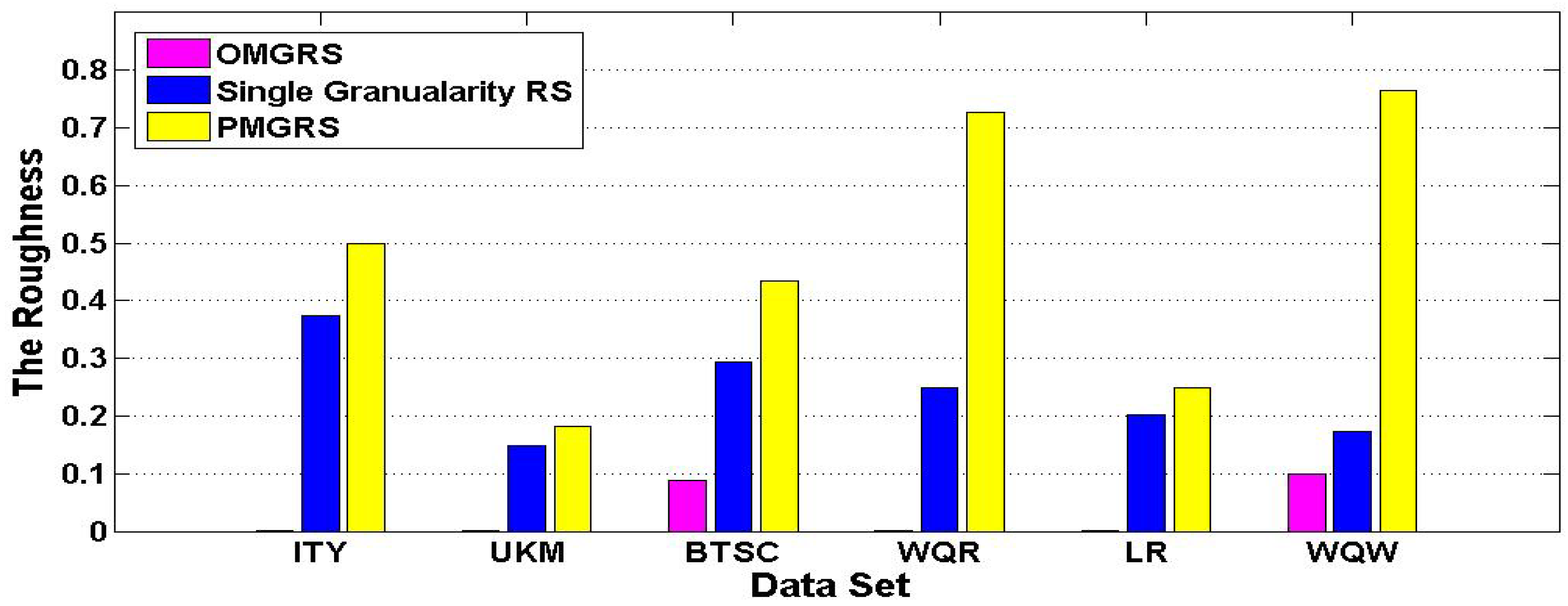
We can draw a histogram Figure 1 based on the results of the roughness in Table 3. As illustrated in Figure 1, the roughness of three rough set models is increasing in each data set according to the order of OMGRS, Single Granularity RS, and PMGRS. Where the roughness in OMGRS is the smallest, the roughness in PMGRS is the largest and the roughness in Single Granularity RS falls in between the roughness in OMGRS and the roughness in PMGRS in each data set, which show the concept become increasingly rough in the light of the order of OMGRS, Single Granularity RS, and PMGRS.
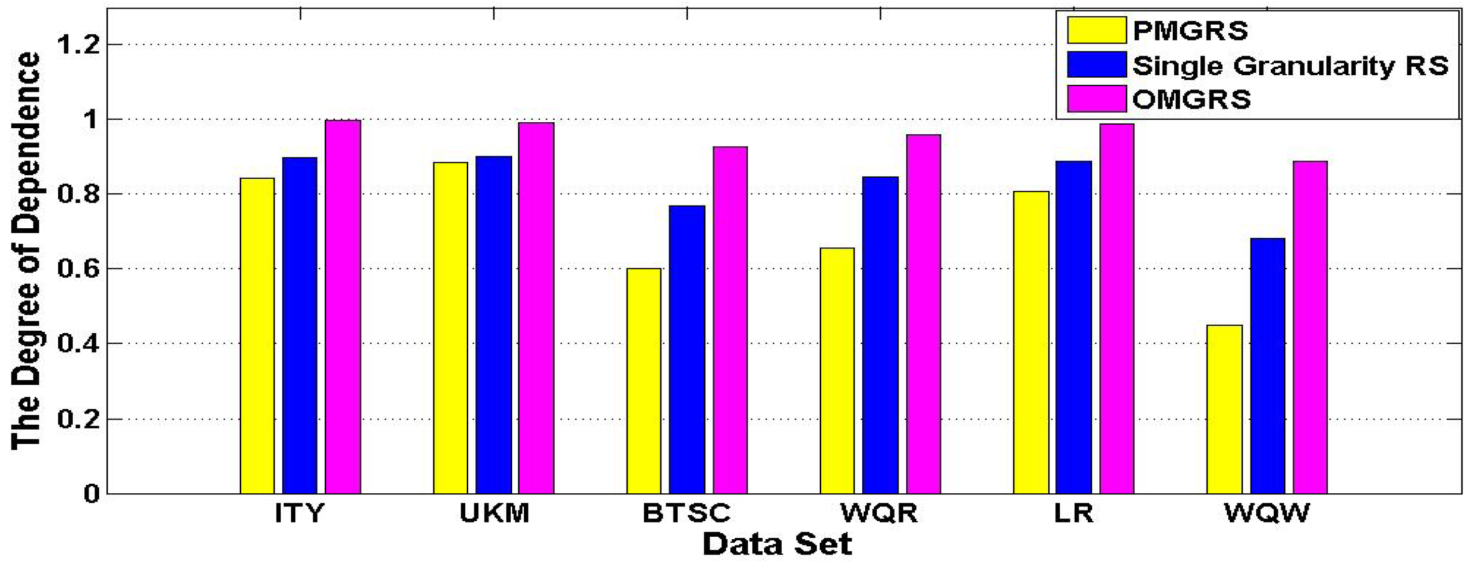
Similarly, we plot the histogram Figure 2 by experimental results about the degree of dependence in Table 3. We can obtain that the degree of dependence of three rough set models is increasing for every data set considering the order of PMGRS, Single Granularity RS, and OMGRS from Figure 2. Where the degree of dependence in PMGRS is the smallest, the degree of dependence in OMGRS is the largest and the degree of dependence in Single Granularity RS falls in between the degree of dependence in PMGRS and the degree of dependence in OMGRS, which reveal the percentage of objects that can be definitely divided into decision classes become increasing in accordance with the order of PMGRS, Single Granularity RS, and OMGRS in every data sets.

7. Conclusions

Multi-granulation rough set has become a hot spot in recent years. In this paper, we define a new relation in the IIVDIS by means of set pair analysis theory, which is the multi-threshold tolerance relation. In this context, we establish single granularity rough set model and two multi-granulation rough set models: the optimistic multi-granulation rough set and the pessimistic multi-granulation rough set. A series of experiments are conducted based on Algorithms 1 and 2 for computing the roughness and the degree of dependence to measure uncertainty of rough set. The results of experiments show the effectiveness and validity of the proposed Theorems. In addition, we can obtain conclusion from Figure 1 and Figure 2:
(1)
The same concept in the PMGRS model is rougher than in the Single Granularity RS. The same concept in the Single Granularity RS model is rougher than in the OMGRS model.
(2)
The degree of dependence represents the percentage of objects, which can definitely divided into decision classes. The percentage in in the OMGRS model is lager than in the Single Granularity RS. The percentage in the Single Granularity RS model is lager than in the PMGRS model.
In the later study, we will mainly analyze other uncertainty measure methods and some reductions based on the MGRS in IIVDIS.

Author Contributions

B.L. is the principal investigator of this work. She performed the experiments and wrote this manuscript. W.X. contributed to the data analysis work and provided several suggestions for improving the quality of this manuscript. All authors revised and approved the publication.

Acknowledgments

This work is supported by the National Natural Science Foundation of China (No. 61472463, No. 61772002, No. 61402064), National Natural Science Foundation of CQ CSTC (cstc2015jcyjA40053), and the Science and Technology Research Program of Chongqing Municipal Education Commission (KJ1709221).

Conflicts of Interest

The authors declare no conflict of interest.

References

  1. Pawlak, Z. Rough sets. Int. J. Comput. Inf. Sci. 1982, 11, 341–356. [Google Scholar] [CrossRef]
  2. Pawlak, Z. Rough set theory and its application to analysis. J. Cybern. 1998, 29, 661–688. [Google Scholar] [CrossRef]
  3. Ahn, B.S.; Cho, S.S.; Kim, C.Y. The integrated methodology of rough set theory and artificial neural network for business failure prediction. Expert Syst. Appl. 2000, 18, 65–74. [Google Scholar] [CrossRef] [Green Version]
  4. Othman, M.L.; Aris, I.B.; Abdullah, S.M.; Othman, M.R. Knowledge discovery in distance relay event report: A comparative data-mining strategy of rough set theory with decision tree. IEEE Trans. Power Deliv. 2010, 25, 2264–2287. [Google Scholar] [CrossRef]
  5. Beaubouef, T.; Ladner, R.; Petry, F.E. Rough set spatial data modeling for data mining. Int. J. Intell. Syst. 2004, 19, 567–584. [Google Scholar] [CrossRef]
  6. Huang, G.B.; Wang, D.H.; Lan, Y. Extreme learning machines: A survey. Int. J. Mach. Learn. Cybern. 2011, 2, 107–122. [Google Scholar] [CrossRef]
  7. Xiao, Q.M.; Zhang, Z.L. Rough prime ideals and rough fuzzy prime ideals in semigroups. Inf. Sci. 2006, 176, 725–733. [Google Scholar] [CrossRef]
  8. Davvaz, B.; Mahdavipour, M. Roughness in modules. Inf. Sci. 2006, 176, 3658–3674. [Google Scholar] [CrossRef]
  9. Kumar, A.; Kumar, D.; Jarial, S.K. A hybrid clustering method based on improved artificial bee colony and fuzzy C-means algorithm. Int. J. Artif. Intell. 2017, 15, 40–60. [Google Scholar]
  10. Wang, C.Z.; Shao, M.W.; He, Q.; Qian, Y.H.; Qi, Y.L. Feature subset selection based on fuzzy neighborhood rough sets. Knowl.-Based Syst. 2016, 111, 173–179. [Google Scholar] [CrossRef]
  11. Wang, C.Z.; Hu, Q.H.; Wang, X.Z.; Chen, D.G.; Qian, Y.H.; Dong, Z. Feature selection based on neighborhood discrimination index. IEEE Trans. Neural Netw. Learn. Syst. 2017, 1–14. [Google Scholar] [CrossRef] [PubMed]
  12. Wang, C.Z.; He, Q.; Shao, M.W.; Hu, Q.H. Feature selection based on maximal neighborhood discernibility. Int. J. Mach. Learn. Cybern. 2017, 1–12. [Google Scholar] [CrossRef]
  13. Zhu, W.; Wang, F.Y. Reduction and axiomization of covering generalized rough sets. Inf. Sci. 2003, 152, 217–230. [Google Scholar] [CrossRef]
  14. Zhang, Q.H.; Xie, Q.; Wang, G.Y. A survey on rough set theory and its applications. CAAI Trans. Intell. Technol. 2016, 1, 323–333. [Google Scholar] [CrossRef]
  15. Zhao, J.Y.; Zhang, Z.L.; Han, C.Z.; Zhou, Z.F. Complement information entropy for uncertainty measure in fuzzy rough set and its applications. Soft Comput. 2015, 19, 1997–2010. [Google Scholar] [CrossRef]
  16. Li, H.X.; Zhou, X.Z.; Zhao, J.B. Non-monotonic attribute reduction in decision-theoretic rough sets. Fundam. Inf. 2013, 126, 415–432. [Google Scholar] [CrossRef]
  17. Wang, C.Z.; He, Q.; Shao, M.W.; Xu, Y.Y.; Hu, Q.H. A unified information measure for general binary relations. Knowl.-Based Syst. 2017, 135, 18–28. [Google Scholar] [CrossRef]
  18. Cheng, Y.; Miao, D.Q. Rule extraction based on granulation order in interval-valued fuzzy information system. Expert Syst. Appl. 2011, 38, 12249–12261. [Google Scholar] [CrossRef]
  19. Zhang, H.Y.; Leung, Y.; Zhou, L. Variable-precision-dominance-based rough set approach to interval-valued information systems. Inf. Sci. 2013, 244, 75–91. [Google Scholar] [CrossRef]
  20. Zhang, J.B.; Li, T.R.; Da, R.; Liu, D. Rough sets based matrix approaches with dynamic attribute variation in set-valued information systems. Int. J. Approx. Reason. 2012, 53, 620–635. [Google Scholar] [CrossRef]
  21. Wang, H.; Yue, H.B.; Chen, X. Attribute reduction in interval and set-valued decision information systems. Appl. Math. 2013, 4, 1512–1519. [Google Scholar] [CrossRef]
  22. Xu, W.H.; Liu, Y.F.; Sun, W.X. Uncertainty measure of Atanassov’s intuitionistic fuzzy T equivalence information systems. J. Intell. Fuzzy Syst. 2014, 26, 1799–1811. [Google Scholar] [CrossRef]
  23. Zhang, X.Y.; Wei, L.; Xu, W.H. Attributes reduction and rules acquisition in an lattice-valued information system with fuzzy decision. Int. J. Mach. Learn. Cybern. 2017, 8, 135–147. [Google Scholar] [CrossRef]
  24. Sowiski, R.; Stefanowski, J. Rough classification in incomplete information systems. Math. Comput. Model. 1989, 12, 1347–1357. [Google Scholar] [CrossRef]
  25. Leung, Y.; Wu, W.Z.; Zhang, W.X. Knowledge acquisition in incomplete information systems: A rough set approach. Eur. J. Oper. Res. 2006, 168, 164–180. [Google Scholar] [CrossRef]
  26. Yang, X.B.; Zhang, M.; Dou, H.L.; Yang, J.H. Neighborhood systems-based rough sets in incomplete information system. Knowl.-Based Syst. 2011, 24, 858–867. [Google Scholar] [CrossRef]
  27. Kryszkiewicz, M. Rough set approach to incomplete information systems. Inf. Sci. 1998, 112, 39–49. [Google Scholar] [CrossRef]
  28. Yang, X.B.; Yu, D.J.; Yang, J.Y.; Wei, L.H. Dominance-based rough set approach to incomplete interval-valued information system. Data Knowl. Eng. 2009, 68, 1331–1347. [Google Scholar] [CrossRef]
  29. Zhang, W.X.; Mi, J.S. Incomplete information system and its optimal selections. Comput. Math. Appl. 2004, 48, 691–698. [Google Scholar] [CrossRef]
  30. Xu, E.S.; Yang, Y.Q.; Ren, Y.C. A new method of attribute reduction based on information quantity in an incomplete system. J. Softw. 2012, 7, 1881–1888. [Google Scholar] [CrossRef]
  31. Wei, L.H.; Tang, Z.M.; Wang, R.Y.; Yang, X.B. Extensions of dominance-based rough set approach in incomplete information system. Autom. Control Comput. Sci. 2008, 42, 255–263. [Google Scholar] [CrossRef]
  32. Yang, X.B.; Qi, Y.; Yu, D.J.; Yu, H.L.; Yang, J.Y. α-Dominance relation and rough sets in interval-valued information systems. Inf. Sci. 2015, 294, 334–347. [Google Scholar] [CrossRef]
  33. Gao, Y.Q.; Fang, G.H.; Liu, Y.Q. θ-Improved limited tolerance relation model of incomplete information system for evaluation of water conservancy project management modernization. Water Sci. Eng. 2013, 6, 469–477. [Google Scholar] [CrossRef]
  34. Yang, X.B.; Yang, J.Y.; Wu, C.; Yu, D.J. Dominance-based rough set approach and knowledge reductions in incomplete ordered information System. Inf. Sci. 2008, 178, 1219–1234. [Google Scholar] [CrossRef]
  35. Shao, M.W.; Zhang, W.X. Dominance relation and rules in an incomplete ordered information system. Int. J. Intell. Syst. 2005, 20, 13–27. [Google Scholar] [CrossRef]
  36. Du, W.S.; Hu, B.Q. Dominance-based rough set approach to incomplete ordered information systems. Inf. Sci. 2016, 346–347, 106–129. [Google Scholar] [CrossRef]
  37. Huang, J.L.; Guan, Y.Y.; Du, X.Z.; Wang, H.K. Decision rules acquisition based on interval knowledge granules for incomplete ordered decision information systems. Int. J. Mach. Learn. Cybern. 2015, 6, 1019–1028. [Google Scholar] [CrossRef]
  38. Dai, J.H.; Wei, B.J.; Shi, H.; Liu, W. Uncertainty measurement for incomplete interval-valued information systems by θ-rough set model. In Proceedings of the 3rd International Conference on Information Management (ICIM), Chengdu, China, 21–23 April 2017; pp. 212–217. [Google Scholar] [CrossRef]
  39. Dai, J.H.; Wei, B.J.; Zhang, X.H.; Zhang, Q.L. Uncertainty measurement for incomplete interval-valued information systems based on α-weak similarity. Knowl.-Based Syst. 2017, 136, 159–171. [Google Scholar] [CrossRef]
  40. Yao, Y.Y. Information granulation and rough set approximation. Int. J. Intell. Syst. 2001, 16, 87–104. [Google Scholar] [CrossRef]
  41. Qian, Y.H.; Liang, J.Y.; Dang, C.Y. Incomplete multigranulation rough set. IEEE Trans. Syst. Man Cybern. Part A 2010, 40, 420–431. [Google Scholar] [CrossRef]
  42. Skowron, A.; Stepaniuk, J. Information granules: Towards foundations of granular computing. Int. J. Intell. Syst. 2001, 16, 57–85. [Google Scholar] [CrossRef]
  43. Xu, W.H.; Zhang, X.Y.; Zhang, W.X. Knowledge granulation, knowledge entropy and knowledge uncertainty measure in ordered information systems. Appl. Soft. Comput. 2009, 9, 1244–1251. [Google Scholar] [CrossRef]
  44. Zadeh, L.A. Toward a theory of fuzzy information granulation and its centrality in human reasoning and fuzzy logic. Fuzzy Sets Syst. 1997, 90, 111–127. [Google Scholar] [CrossRef]
  45. Qian, Y.H.; Liang, J.Y.; Yao, Y.Y.; Dang, C.Y. MGRS: A multi-granulation rough set. Inf. Sci. 2010, 180, 949–970. [Google Scholar] [CrossRef]
  46. Medina, J.; Ojeda-Aciego, M. Multi-adjoint t-concept lattices. Inf. Sci. 2010, 180, 712–725. [Google Scholar] [CrossRef]
  47. Pozna, C.; Minculete, N.; Precup, R.E.; Kóczy, L.T.; Ballagi, Á. Signatures: Definitions, operators and applications to fuzzy modelling. Fuzzy Sets Syst. 2012, 201, 86–104. [Google Scholar] [CrossRef]
  48. Nowaková, J.; Prílepok, M.; Snášel, V. Medical image retrieval using vector quantization and fuzzy S-tree. J. Med. Syst. 2017, 41, 1–16. [Google Scholar] [CrossRef] [PubMed]
  49. Zhang, M.; Xu, W.Y.; Yang, X.B.; Tang, Z.M. Incomplete variable multigranulation rough sets decision. Appl. Math. Inf. Sci. 2014, 8, 1159–1166. [Google Scholar] [CrossRef]
  50. Yang, W. Interval-valued information systems rough set model based on multi-granulations. Inf. Technol. J. 2013, 12, 548–550. [Google Scholar] [CrossRef]
  51. Xu, W.H.; Sun, W.X.; Zhang, X.Y.; Zhang, W.X. Multiple granulation rough set approach to ordered information systems. Int. J. Gen. Syst. 2012, 41, 475–501. [Google Scholar] [CrossRef]
  52. Wang, L.J.; Yang, X.B.; Yang, J.Y.; Wu, C. Incomplete multigranulation rough sets in incomplete ordered decision system. In Bio-Inspired Computing and Applications; Huang, D.S., Gan, Y., Premaratne, P., Han, K., Eds.; Springer: Berlin/Heidelberg, Germany, 2012; Volume 6840, pp. 323–330. ISBN 978-3-642-24552-7. [Google Scholar]
  53. Yang, X.B.; Song, X.N.; Chen, Z.H.; Yang, J.Y. On multigranulation rough sets in incomplete information system. Int. J. Mach. Learn. Cybern. 2012, 3, 223–232. [Google Scholar] [CrossRef]
  54. Zhao, K.Q. Set pair analysis and prelimiary application. Explor. Nat. 1994, 13, 67–72. (In Chinese) [Google Scholar]
  55. Chen, Z.C.; Qin, K.Y. Attribute reduction of interval-valued information system based on variable precision tolerance relation. Comput. Sci. 2009, 36, 163–166. (In Chinese) [Google Scholar]
  56. Zeng, L.; He, P.Y.; Fu, M. Attribute reduction algorithm based on rough set in incomplete interval-valued information. J. Nanjing Univ. Sci. Technol. 2013, 37, 524–529. (In Chinese) [Google Scholar]
Figure 1. The roughness of three rough sets.
Symmetry 10 00208 g001
Figure 2. The degree of dependence about three rough sets.
Symmetry 10 00208 g002
Table 1. An Incomplete Interval-valued Decision Information System.
U a 1 a 2 a 3 a 4 a 5 a 6 a 7 d
x 1 [ 1.90 , 2.10 ] [ 31.35 , 34.65 ] **** [ 23.75 , 26.25 ] 1
x 2 [ 0.95 , 1.05 ] [ 23.75 , 26.25 ] [ 5.4625 , 6.0375 ] [ 1.90 , 2.10 ] [ 0.95 , 1.05 ] [ 285 , 315 ] [ 6.65 , 7.35 ] 1
x 3 [ 1.90 , 2.10 ] *** [ 0.95 , 1.05 ] [ 28.50 , 31.50 ] [ 2.85 , 3.15 ] 1
x 4 [ 1.90 , 2.10 ] [ 45.60 , 50.40 ] [ 9.7375 , 10.7625 ] [ 6.65 , 7.35 ] * [ 47.50 , 52.50 ] [ 23.75 , 26.25 ] 1
x 5 [ 0.95 , 1.05 ] [ 31.35 , 34.65 ] [ 1.6625 , 1.8375 ] [ 6.65 , 7.35 ] [ 1.90 , 2.10 ] [ 360.05 , 397.95 ] [ 6.65 , 7.35 ] 0
x 6 [ 1.90 , 2.10 ] [ 36.10 , 39.90 ] [ 2.3750 , 2.6250 ] [ 0.95 , 1.05 ] * [ 40.85 , 45.15 ] [ 47.50 , 52.50 ] 1
x 7 [ 0.95 , 1.05 ] * [ 9.500 , 10.5000 ] ****1
x 8 * [ 22.80 , 25.20 ] [ 4.0375 , 4.4625 ] [ 0.95 , 1.05 ] [ 0.95 , 1.05 ] * [ 28.50 , 31.50 ] 1
x 9 [ 0.95 , 1.05 ] [ 18.05 , 19.95 ] [ 7.3625 , 8.1375 ] * [ 0.95 , 1.05 ] * [ 6.65 , 7.35 ] 1
x 10 [ 0.95 , 1.05 ] [ 32.30 , 35.70 ] * [ 6.65 , 7.35 ] * [ 60.80 , 67.20 ] [ 6.65 , 7.35 ] 0
x 11 [ 0.95 , 1.05 ] [ 27.55 , 30.45 ] [ 4.7500 , 5.2500 ] [ 11.40 , 12.60 ] [ 2.85 , 3.15 ] [ 71.25 , 78.75 ] [ 6.65 , 7.35 ] 1
x 12 [ 0.95 , 1.05 ] * [ 2.1375 , 2.3625 ] * [ 2.85 , 3.15 ] [ 48.45 , 53.55 ] *1
x 13 [ 0.95 , 1.05 ] [ 43.70 , 48.30 ] * [ 3.80 , 4.20 ] * [ 86.45 , 95.55 ] [ 23.75 , 26.25 ] 0
x 14 ***** [ 82.65 , 91.35 ] [ 5.70 , 6.30 ] 0
x 15 [ 0.95 , 1.05 ] * [ 10.6875 , 11.8125 ] * [ 0.95 , 1.05 ] [ 68.40 , 75.60 ] *0
x 16 * [ 16.15 , 17.85 ] [ 8.0750 , 8.9250 ] [ 1.90 , 2.10 ] ** [ 7.60 , 8.40 ] 1
x 17 ** [ 4.7500 , 5.2500 ] [ 1.90 , 2.10 ] [ 0.95 , 1.05 ] * [ 4.75 , 5.25 ] 1
x 18 [ 1.90 , 2.10 ] [ 21.85 , 24.15 ] [ 6.4125 , 7.0875 ] [ 5.70 , 6.30 ] [ 0.95 , 1.05 ] ] * [ 1.90 , 2.10 ] 1
x 19 * [ 34.20 , 37.80 ] [ 1.6625 , 1.8375 ] * [ 2.85 , 3.15 ] [ 42.75 , 47.25 ] [ 2.85 , 3.15 ] 1
x 20 [ 0.95 , 1.05 ] [ 36.10 , 39.90 ] [ 7.1250 , 7.8750 ] [ 7.60 , 8.40 ] [ 1.90 , 2.10 ] [ 53.20 , 58.80 ] [ 42.75 , 47.25 ] 1
Table 2. The testing data sets.
Data SetsAbbreviationObjectAttributeDecision Class
ImmunotherapyIMY9082
User Knowledge ModelingUKM40364
Blood Transfusion Service CenterBTSC74852
Wine Quality-RedWQR1599126
Letter RecognitionLR34001626
Wine Quality-WhiteWQW4898127
Table 3. The computation results both Algorithms 1 and 2 in IIVDIS.
Data SetsThe RoughnessThe Degree of Dependence
OMGRSSingle Granularity RSPMGRSPMGRSSingle Granularity RSOMGRS
IMY0.00010.37500.50000.84440.90001.0000
UKM0.00010.14810.18180.88590.90070.9926
BTSC0.08880.29350.43440.60160.76870.9278
WQR0.00010.25000.72730.65670.84620.9581
LR0.00010.20130.24850.80710.88850.9894
WQW0.10000.17390.76470.45040.68190.8887

