Article

A Synthetic Fusion Rule for Salient Region Detection under the Framework of DS-Evidence Theory

1
School of Computer Science and Technology, Dalian University of Technology, Dalian 116024, China
2
College of Computer Science and Technology, Huaqiao University, Xiamen 361021, China
3
School of Computer Science and Technology, Shandong University of Finance and Economics, Jinan 250100, China
*
Authors to whom correspondence should be addressed.
Symmetry 2018, 10(6), 183; https://doi.org/10.3390/sym10060183
Submission received: 26 April 2018 / Revised: 17 May 2018 / Accepted: 23 May 2018 / Published: 25 May 2018

Abstract

:
Saliency detection is one of the most valuable research topics in computer vision. It focuses on the detection of the most significant objects/regions in images and reduces the computational time cost of getting the desired information from salient regions. Local saliency detection or common pattern discovery schemes were actively used by the researchers to overcome the saliency detection problems. In this paper, we propose a bottom-up saliency fusion method by taking into consideration the importance of the DS-Evidence (Dempster–Shafer (DS)) theory. Firstly, we calculate saliency maps from different algorithms based on the pixels-level, patches-level and region-level methods. Secondly, we fuse the pixels based on the foreground and background information under the framework of DS-Evidence theory (evidence theory allows one to combine evidence from different sources and arrive at a degree of belief that takes into account all the available evidence). The development inclination of image saliency detection through DS-Evidence theory gives us better results for saliency prediction. Experiments are conducted on the publicly available four different datasets (MSRA, ECSSD, DUT-OMRON and PASCAL-S). Our saliency detection method performs well and shows prominent results as compared to the state-of-the-art algorithms.

1. Introduction

Nowadays, images are becoming an important piece of media for information transmission, information retrieval and information security. Saliency information extraction from images is one of the most active research area in the field of computer and robotics vision. Due to a large amount of data, it is difficult to deal with the large number of images quickly and accurately. The task of image saliency detection is to determine the areas of focus by the human visual system in images and videos. There are different important aspects that should be considered for extracting saliency information from images like motion, depth, color and localization factors, etc. If the salient parts are extracted accurately, the calculation time could be significantly reduced and fast processing of images can be realized. The idea of saliency detection was first introduced by Itti et al. [1]. At present, applications of image saliency detection are very successful in images transmission systems [2], image quality assessment [3], image compression [4], image segmentation [5], target recognition [6], image scaling [7], image retrieval [8], foot plant detection [9], and other areas as well.
Several saliency detection methods have been introduced to overcome the problems in computer vision system for the last three decades. Some methods solely concentrate on low level visual cues for saliency information extraction. These methods can be categorized into pixels-based, patches-based and region-based methods. A seminal pixel-based saliency detection method was introduced by Itti et al. [1] in which saliency information was obtained from pixel-level features and center-surround differences. Achanta et al. [10] adopted a saliency detection approach based on the frequency features of the images by exploiting the pixel-wise difference with mean shift segmentation and calculate the saliency by disregarding high frequencies arising from texture, noise on each pixel. These methods have some shortcomings like boundary blurring, and poorly segmenting the salient object due to the interior suppression. Due to these shortcomings of pixel-based methods, researchers introduced a patch level saliency detection method. Margolin et al. [11] proposed a method in which they used the Principal Component Analysis to represent the set of patches and ignored all of other patches in the image. Recently, Wang et al. [12] proposed a method based on scene-level analysis and patch-level inference to support nearest semantics to get saliency information. However, they used region based segmentation of image patches and made use of other cues to refine the saliency detection. They also used the scene-level analysis with patch-level to overcome the inefficiency of the patch-level based methods. In other words, pure patch-based methods cannot achieve satisfying results.
In contrast to overcoming the patches and pixels based saliency detection methods, region based saliency detection methods have been introduced. In region-based methods, images are segmented according to the region-level. Due to irregular regions in some images, those methods can be sub-categorized and explored on the base of the regions with irregular sizes and shapes [13,14,15,16] and regions with regular sizes and shapes [17,18,19,20,21]. Wei et al. [13] introduced a region-based saliency detection method by focusing on the background more than the salient region and exploited two common priors about backgrounds boundary and connectivity priors. Perazzi et al. [14] proposed getting saliency information by decomposing the given image into a group of homogeneous elements and generating a pixel-wise saliency map. Cheng et al. [15] used pixels’ appearance information based on the spatial distribution and similarity for salient region detection. Cheng et al. [16] evaluated the saliency with spatial weighted coherence scores and global contrast differences, which gives prominent results, but this method can not perform well in all cases. Achanta et al. [17] introduced a simple linear iterative clustering (SLIC) super-pixel method for segmenting the salient region based on mid-level visual features. The absorption Markov chain has been used by Jiang et al. [18] in which the transient nodes on the image boundaries are computed first and absorbing nodes are treated as virtual boundary nodes for estimation of the salient regions based on the background and foreground. Yang et al. [19] used a method for saliency estimation by treating super-pixels as nodes and these nodes are divided into subsets of similarity to background and foreground queries. Hence, saliency is computed based on the two non-overlapping regions, as background and salient region. Xie et al. [20] also used the low and mid-level visual features of the image to define the regions as background and foreground. In this method, firstly, the salient region is estimated via color features and foreground region is defined using convex hull. Secondly, super-pixels are used to define salient regions based on the mid-level visual features. Following Xie’s saliency detection framework, Ayoub et al. [21] also employed Bayesian framework for saliency detection. They calculated color frequency features of the images by employing Log–Gabor filter and calculated the salient region by splitting the regions into foreground and background with convex hull. This method shows prominent results as compared to the rest of the methods, but, as it uses color features, this method can not perform on gray scale images.
Almost all methods have their importance in conducting image saliency, but, due to the use of the pixels’, patches’ and region based information, these methods cannot perform well in all cases. Even different saliency detection methods are complemented to each other [22]. Therefore, fusing saliency maps of predefined functions based on the pixels’, patches’ and regional-level information gives impressive results. For better saliency estimation, in this paper, we introduce a new method to fuse different saliency maps obtained by different predefined algorithms, based on the color, motion, depth, patches, pixels and regional level information with Dempster–Shafer (DS)-Evidence theory. In this paper, the remaining sections are organized as follows. The related work based on pixel-level, patch-level and region-level saliency detection methods is described in Section 2 (Related Work). Section 3 (Proposed algorithm) elaborates on the two major steps. Firstly, a review of the DS-Evidence theory is described. Secondly, we briefly discuss our proposed approach together with the summary of the complete algorithm. Illustration and experimental results on four different datasets are presented in Section 4. Finally, the conclusions are made in Section 5.
Figure 1 shows the pipeline of proposed (DS-OUR) saliency fusion framework.

2. Related Work

Various saliency computational models are based on the structure of Feature Integration Theory [23]. In this theory, objects are supposed to be attentive in a visual scene by its shape, color and orientations, etc., and are focused by combining these features. Itti et al. [1] practically implemented these features for the first time to construct the saliency map. Some researchers used pixel-wise local priors for saliency detection. Lu et al. [24] calculated pixel-level saliency by integrating multi-scale reconstruction errors and a Gaussian model to refine them under Bayesian framework. Seo et al. [25] calculated the pixel-level saliency by processing each pixel to its surroundings. Perazzi et al. [14] introduced a pixel level saliency detection method in which an image was decomposed into compact and homogeneous elements to extract the necessary detail; then, the uniqueness and the spatial distribution of these elements are measured to estimate saliency information.
Researchers also used patches level information to estimate the region of interest. Shi et al. [26] used image patches to tackle the saliency problem and introduced a new saliency benchmark data-set (ECSSD). They also proposed a multi-layer approach for saliency map construction. The saliency information extracted a hierarchical model of three layers of different patch sizes, and these layers are then combined together to produce the final saliency map. Tong et al. [27] used a multi-scale saliency detection method. They segmented the image into multi-scale super-pixels and then estimated three different cues from integrity, contrast and central biased on each scale within the Bayesian framework for saliency detection. They used a guided filter to smooth the final saliency map obtained by a summation of the saliency information.
Some researchers computed the saliency maps from regional level information by segmenting the images into foreground and background. Wei et al. [13] proposed a region based geodesic saliency detection method in which a saliency map is produced by taking into account the probability of the background priors as boundary and connectivity priors. A graph based saliency detection method was introduced by Yang et al. [19] in which a region level saliency detection method is proposed by representing the image as a close-loop graph with super-pixels as nodes. Then, background and foreground based nodes are ranked together to estimate the salient region based on affinity matrices. Xie et al. [20] proposed a regional level saliency method based on Bayesian framework. They calculated a saliency map by using low and mid level visual cues. Firstly, saliency information is extracted using color priors and then a convex hull is computed to estimate foreground and background. The saliency map is then computed pixel-wise inside and outside the convex hull under the Bayesian framework. By taking into consideration the importance of Bayesian framework, Ayoub et al. [21] calculated the saliency map by using color and texture features of images. They used Bayesian framework to estimate the salient region. Zhu et al. [28] proposed a well modeled saliency detection method in which image boundary regions were characterized in spatial layout by taking into considerations the robust background measure, called boundary connectivity. Secondly, an optimization framework was used for integration of low level visual cues.
DS-Evidence theory is more applicable for the saliency fusion than other saliency fusion methods. DS-Evidence theory is based on Dempster’s work [29] of upper and lower probabilities. The use of belief functions into the artificial intelligence was introduced by Barnett [30] in which he introduced the degree of belief function as a numerical method that combines all possible evidences instead of null hypothesis. Lowrance et al. [31] defined the DS-Evidence functions as evidential-reasoning which manipulate all possible reasoning of evidence. A lot of work has been done to improve the DS-Evidence theory to get the maximum information from the input data. Various methods for saliency estimation have improved the results of saliency maps for good in accuracy and recall rate. It is much better to fuse all possible evidence of saliency values rather than a single probability value to reach on the degree of acceptance. The importance of the DS-Evidence theory and its use in fusing all of the possible outcomes instead of a null hypothesis can increase the effect of saliency estimation higher than that of each individual saliency detection method.
Figure 2 shows the comparison of saliency maps calculated from our algorithm and nine other state-of-the-art saliency detection algorithms.

3. Proposed Algorithm

3.1. DS-Evidence Theory Review

DS-Evidence theory was proposed in 1967 by Dempster [29] in which Dempster introduced a system of upper and lower probabilities. In the context of statistical inference, Shafer developed the theory for uncertainty modeling frameworks in 1976 [32]. Beynon et al. [33] revealed that the DS-Evidence theory has numerous advantages over the various statistical methods and Bayesian decision theory due to its performance in modeling the reasons under uncertainty. The DS-Evidence theory can be defined as follows:
Denoting the universal set by Θ , which represents a finite set of all possible hypotheses of a problem and its power set by 2 Θ to quantify the candidate proposition. The basic probability assignment (BPA) m : 2 Θ [ 0 , 1 ] can be defined as
m ( ϕ ) = 0 , A 2 Θ m ( A ) = 1 .
A probability of mass m ( A ) provides the body of confidence that proposition A is true. Any set A 2 Θ that possesses a nonzero BPA, where m ( A ) > 0 is called a focal element. In the formalism, the imprecision of knowledge can be handled by assigning a nonzero probability mass to the union of two or more classes.
The rule proposed by Dempster played an important role in DS-Evidence theory. Given M mass functions as m 1 , m 2 , , m M , the rule is defined as
( m 1 m M ) ( A ) = 1 1 A 1 A M = A i = 1 M m i ( A i ) ,
where A i 2 Θ , 1 i M and can be calculated as
= A 1 A M i = 1 M m i ( A i ) .
The property of DS-Evidence theory of combining evidence from different sources makes it applicable for dealing with reasoning under uncertain conditions. The probability can be assigned to any of the subsets of the discernment framework without having the condition to be mutually exclusive and exhaustive. DS-Evidence theory regards each subset as a single hypothesis, which can simulate the reasoning similar to human logic. Therefore, DS-Evidence theory is more applicable in fusion tasks.

3.2. DS-Fusion Method

We propose a method for saliency maps fusion based on DS-Evidence theory with the aim to overcome the shortcomings of the above-mentioned prior state-of-the-art methods.
In the first step, n pieces of initial saliency images are generated using n ( n > 1 ) methods to be fused. In our experiments, we used nine different saliency detection methods, n = 9.
In the second step, for each pixel, we define the mass function corresponding to the n saliency images. Define the environment Θ = { F G , B G } where F G represents the pixel as the foreground and B G represents the pixel as the background. The recognition framework contains 2 2 subset, which defines a set of powers that can represent pixels as a foreground or a background as 2 Θ . We know that the mass function is satisfied when Σ A 2 Θ m ( X ) = 1 . Thus, we can define the mass function (basic trust assignment function) in the form of n saliency images as shown in Equations (4) and (5):
m i ( F G ) = P i ,
m i ( B G ) = 1 P i ,
where m i ( F G ) represents the mass function corresponding to the i th saliency maps. F G indicates that the pixels that should be fused are in the foreground and the saliency value at the corresponding pixel. B G indicates that the corresponding pixel is in the background.
In the third step, we calculate the similarity coefficients between the mass functions corresponding to each saliency images (i.e., each piece of evidence), and list the similar matrices. The similarity coefficient is calculated by Equation (6):
d i j = A x B y 0 m i ( A x ) m j ( B y ) ( m i 2 ( A x ) ) ( m j 2 ( B y ) ) ,
where the similarity coefficient d i j ( d i j [ 0 , 1 ] ) is used to describe the degree of similarity between the evidence. d i j = 1 indicates the similarity between two pieces of evidence and d i j = 0 indicates that two pieces of evidence are completely different. From the correlation coefficient, we can get the similarity matrix corresponding to n evidence by Equation (7):
S = 1 d 12 . . . d 1 n d 21 1 . . . d 2 n . . . . . . . . . . . . . . . . . . d n 1 d n 2 . . . 1 n × n
In the fourth step, we find the supported level and credibility among the evidence. The degree of support of the evidence indicates the degree of support by other evidence, and if one piece of evidence are similar to other evidence. The mutual support is considered to be higher and the support formula of the evidence is shown in Equation (8):
S U P ( m i ) = j = 1 n d i j ( i , j = 1 , 2 , , n ) .
The credibility of the evidence reflects the credibility of the general evidence of a higher degree. Credibility can be calculated as follows:
C r d ( m i ) = s u p ( m i ) i = 1 n s u p ( m i ) .
In the fifth step, with the credibility as the weight of the mass function, we get the weighted mass function m a v e ( F G ) by taking the pixel as the basic probability of the foreground assignment by Equation (10).
m a v e ( F G ) = i = 1 n C r d ( m i ) × m i ( F G ) .
In addition, here we will use the weighted mass function value as the saliency value of the saliency image. All possible prospects of saliency image can detect effectively by a preliminary synthesis of a significant map. We can assume the m a v e ( F G ) as an initial saliency map with the foreground pixels:
s a l 1 = m a v e ( F G ) .
In the sixth step, the weighted average evidence is used for n 1 times in the DS synthesis rule to obtain another saliency image of fusion. We know that DS-Evidence mass function in the synthesis of the law Equation (2). We can get the synthetic mass function as shown in Equation (12):
m ( F G ) = ( m a v e ( F G ) ) n k ,
where k = ( m a v e ( F G ) ) n + ( 1 m a v e ( F G ) ) n .
Here, we can get another saliency image s a l 2 by Equation (13)
s a l 2 = m ( F G ) .
In the seventh step, we calculate the weighted fusion of the intial saliency maps s a l 1 and s a l 2 . The final saliency map can be calculated by merging both intial saliency maps with different weights as follows:
s a l = μ 1 × s a l 1 + μ 2 × s a l 2 ,
where μ 1 , μ 2 are the composition weights. We set μ 1 = 0.35 and μ 2 = 0.65 in our experimental work.
The method is different from the existing methods because it takes advantage of the various saliency detection methods and the results are superior to the results of each individual saliency detection method. Initial saliency maps can be merged by giving the different weights. Comparison with the traditional methods shows that the proposed method (DS-OUR) outperforms the various saliency detection methods. The complete algorithm of proposed saliency fusion method is summarized in Algorithm 1.
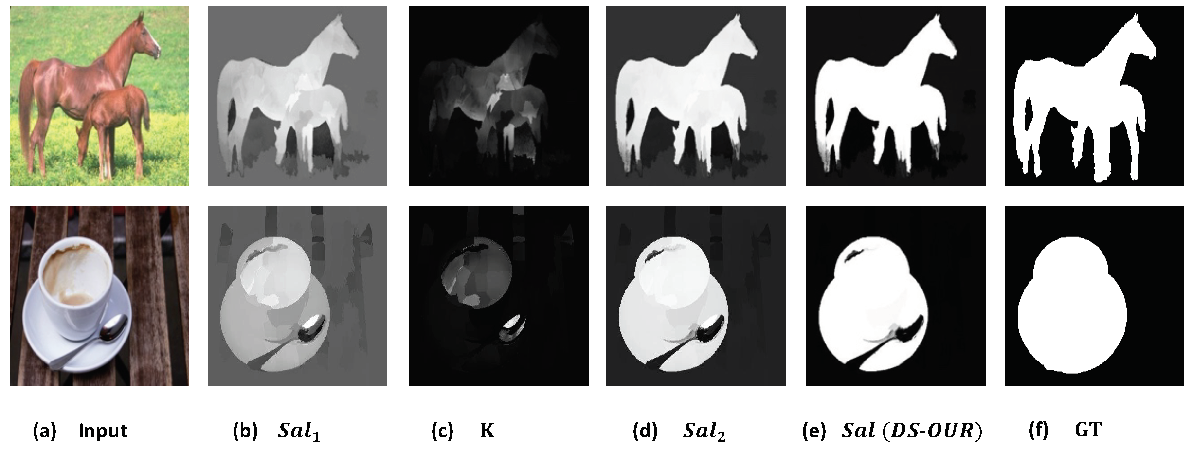
Figure 3 shows the saliency maps results calculated by Equations (11), (13) and (14).
Algorithm 1: DS-Saliency Fusion Algorithm
Symmetry 10 00183 i001

4. Experiments and Results

4.1. Data-Sets

For the evaluation purposes, we use four publicly available datasets in contrast to the efficiency comparison of our algorithm against nine state-of-the-art saliency detection models. These datasets have been used by many researchers in their articles to predict and estimate the efficiency of their algorithms.
MSRA consists of 1000 images introduced by Achanta et al. [10]. It contains pixel-wise ground truth masks of the salient object annotation in terms of bounding boxes, annotated by 3–9 users. It is one of the widely used datasets by the Computer vision community for saliency detection and segmentation comparisons.
ECSSD was introduced by Shi et al. [26] as an extended version of CSSD dataset and contains 1000 images acquired from the Internet. The images in ECSSD dataset structurally have a more complex background than the CSSD dataset. Pixel-wise ground truth masks were annotated by five different users for this dataset.
DUT-OMRON was introduced by Yang et al. [19]. It consists of 5168 high quality images, manually selected from more than 140,000 images. These Images contain one or more salient objects with complex background. Pixel-wise ground truth masks in terms of bounding boxes were annotated by 25 users.
PASCAL-S was built on the validation set of the PASCAL-S segmentation challenge introduced by Li et al. [34]. It contains 850 natural images as a subset of the PASCAL VOC dataset, with both saliency segmentation ground truth and eye fixation ground truth. The PASCAL-S is a less biased data-set and contains one or more objects. Pixel-wise ground truth masks were annotated by 12 users for this dataset.
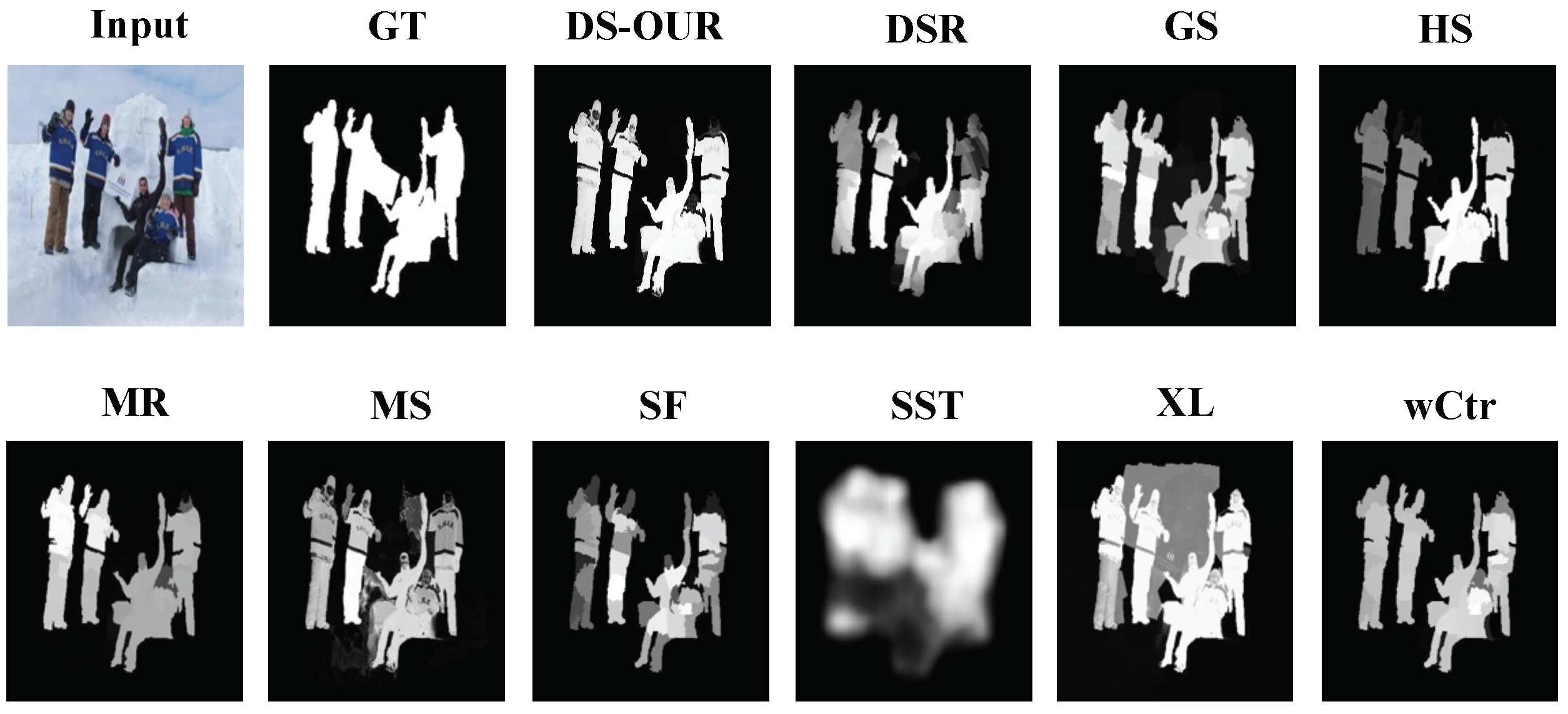
Figure 4 shows the saliency maps calculated by our saliency detection method and nine different state-of-the-art algorithms on four different data-sets.

4.2. Evaluation Metrics

We follow the evaluation matrices used in [10,19,20,26], where saliency maps are binarized at a fixed threshold within range [0, 255].

4.2.1. Precision–Recall Curves

Precision–Recall curves are used to evaluate the performance in contrast to the best estimation of salient regions. Many researchers have employed the method Precision–Recall matrices to show the accuracy of their algorithms, where saliency maps are binarized within the domain of [0, 255] and compared with the ground truth fixation masks. The thresholds vary from 0 to 255 and precision_recall metrics are calculated at each binarized threshold by Equation (15)
P r e c i s i o n = t n p s n p , R e c a l l = t n p g n p ,
where t n p is the total number of the pixels inside the salient regions of the saliency map and ground truth, s n p , is the number of the salient pixels in saliency map. g n p , is the number of the salient pixels inside the salient region of ground truth.

4.2.2. ROC–AUC Curves

Receiver Operating Characteristic (ROC) curves are used to quantify the performance of a saliency map detection algorithm in contrast to distinguishing fixation vs. non-fixation regions. AUC stands for the area under the ROC curve. The greater value of the AUC shows the better performance of the classifier. The value of AUC is calculated based on a true positive rate (TPR) and a false positive rate (FPR). TPR is the ratio of the number of saliency values above a given threshold that overlap with the fixation points in the ground truth. FPR is the ratio of the number of saliency map values above the given threshold that do not overlap with the fixation points in the ground truth map. TPR and FPR are computed as follows:
T P R = T P T P + F N , F P R = F P F P + T N .
Figure 5 shows the AUC comparison results on four different datasets. Our saliency detection method performs well with higher AUC values.

4.2.3. F-Measure

F-measure scores are calculated as a harmonic mean of average precision and average recall. We set α 2 to 0.3 to weigh precision more than recall. The precision, recall and F-measure are averaged over total number of the images:
F = ( 1 + α 2 ) p r e c i s i o n × r e c a l l α 2 × p r e c i s i o n + r e c a l l ,
where value of α 2 is 0.3.
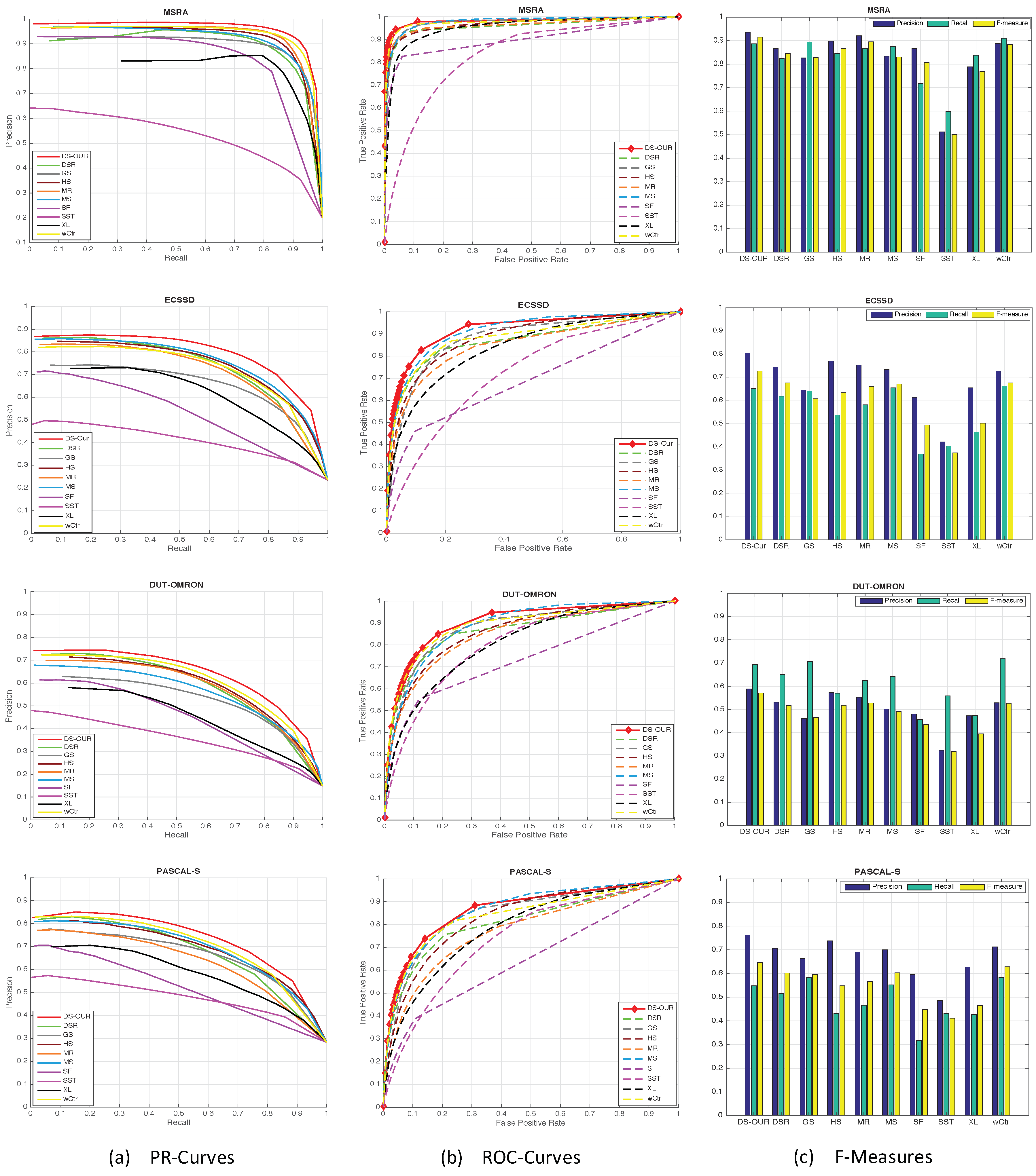
Figure 6 shows the graphical representation of precision–recall curves, ROC curves and F-measures comparison results on the databases presented in [10,19,26,34].

4.2.4. MAE Evaluation

Mean Absolute Error (MAE) is used to measure the closed prediction between calculated saliency map and ground truth map. MAE is computed between saliency map (S) and Ground truth (G). The formula for measuring mean absolute error is
M A E = 1 n i = 1 n S m a p ( i ) G m a p ( i ) .
Figure 7 shows the MAE comparison results on four different data-sets. Our saliency detection method shows better performance against other saliency detection by showing a minimum mean absolute error.

4.3. Performance Comparison

For the evaluation purposes, we compare the quantitative and qualitative results obtained from our method and nine different state-of-the-art algorithms. We compare our saliency maps’ results in contrast to better object detection in the images. The method XL [20] detects non-interesting background pixels as salient, and it calculates saliency of each pixel inside and outside the interesting region by using the convex-hull method with low level visual features. This method can not perform well when the same color of the background is detected as foreground. The approach SF [14] fails to detect the salient pixels of the prominent objects as it considers the saliency as uniqueness of the pixels and spacial distribution of the elements. Our approach consistently estimates the accurate pixels on the dominant objects and their contextual surroundings by considering the pixels of foreground and background, and fuse them for better results. Our final saliency maps were computed by fusing the saliency maps by using Equation (14). We took two sample images from each database presented in [10,19,26,34]. These databases contain the original images and annotated ground-truths to show the saliency maps’ comparison results. Figure 4 shows the comparison of our saliency maps results with the biologically-inspired saliency detection approaches. Our algorithm gives the better performance in contrast to over all thresholded accuracy. Figure 5 shows the AUC comparison results on four different datasets. Our saliency detection method performs well with higher AUC values. Figure 6 shows the graphical representation of precision–recall curves, ROC curves and F-measures comparison results. Figure 7 shows the graphical representation of MAE (Mean absolute error) results on the four different data-sets, our (DS-OUR) algorithm shows minimum error in contrast to overall performance in saliency detection as compared to the other nine state-of-the-art algorithms. In part of the images, only the prominent object was marked. For the purpose of fair evaluation, we performed the experiments on these datasets with each algorithm. Table 1 shows quantitative comparison of our algorithm against nine state-of-the-art algorithms. The quantitative results obtained from our algorithm shows the best performance in terms of the AUC (Maximum is better), MAE (Minimum is better) and F-measure values (maximum is better).

5. Conclusions

In this paper, we discuss the DS-Evidence theory that is used to fuse the saliency maps in our proposed method. Second, our method regards the saliency information extraction as an important issue and considers the foreground and background regions to get the salient pixels’ information. Inspired by processes of the human visual and cognitive systems, our proposed method uses the relationship model between saliency labels. We calculate saliency maps by adopting different methods, based on the pixels-level, patches-level and regional-level information. We fuse these saliency maps under the framework of DS-Evidence theory. Extensive experiments on four publicly available images data-sets demonstrate that the proposed method significantly outperforms state-of-the-art saliency detection methods, particularly in terms of insensitivity to different features. In the future, we plan to improve our proposed framework for saliency detection by adding noise and incomplete scenes.

Author Contributions

N.A. is a scholar under supervisor Z.G. and co-supervisor B.C. conducted this research work. N.A. and Z.G. conceived and designed the proposed saliency detection model. N.A. finalized the theoretical framework and performed the simulation-based experiments. M.J. provided the suggestions on the algorithm, analyzed the simulations’ results and validated the performance achievements by comparing results with existing material. N.A. and Z.G. completed the write-up process and B.C. completed the critical revisions.

Funding

This research was funded by [National Natural Science Foundation of China] grant number [61671169].

Conflicts of Interest

The authors declare no conflict of interest.

References

  1. Itti, L.; Koch, C.; Niebur, E. A model of saliency-based visual attention for rapid scene analysis. IEEE Trans. Pattern Anal. Mach. Intell. 1998, 20, 1254–1259. [Google Scholar] [CrossRef]
  2. Zhao, J.; Liu, X.; Sun, J.; Zhou, S. Imaging of Transmission Equipment by Saliency-Based Compressive Sampling. In Proceedings of the 2012 International Conference on Information Technology and Software Engineering, Beijing, China, 8–10 December 2012; Springer: Berlin/Heidelberg, Germany, 2013; pp. 689–696. [Google Scholar] [CrossRef]
  3. Gu, K.; Wang, S.; Yang, H.; Lin, W.; Zhai, G.; Yang, X.; Zhang, W. Saliency-Guided Quality Assessment of Screen Content Images. IEEE Trans. Multimed. 2016, 18, 1098–1110. [Google Scholar] [CrossRef]
  4. Harding, P.; Robertson, N.M. Visual Saliency from Image Features with Application to Compression. Cognit. Comput. 2013, 5, 76–98. [Google Scholar] [CrossRef] [Green Version]
  5. Sima, H.; Liu, L.; Guo, P. Color Image Segmentation Based on Regional Saliency. In Neural Information Processing; Springer: Berlin/Heidelberg, Germany, 2012; pp. 142–150. [Google Scholar] [CrossRef]
  6. Li, L.; Ren, J.; Wang, X. Fast cat-eye effect target recognition based on saliency extraction. Opt. Commun. 2015, 350, 33–39. [Google Scholar] [CrossRef]
  7. Jia, S.; Zhang, C.; Li, X.; Zhou, Y. Mesh resizing based on hierarchical saliency detection. Graph. Model. 2014, 76, 355–362. [Google Scholar] [CrossRef]
  8. Yang, X.; Qian, X.; Xue, Y. Scalable Mobile Image Retrieval by Exploring Contextual Saliency. IEEE Trans. Image Process. 2015, 24, 1709–1721. [Google Scholar] [CrossRef] [PubMed]
  9. Lu, J.; Liu, X. Foot plant detection for motion capture data by curve saliency. In Proceedings of the Fifth International Conference on Computing, Communications and Networking Technologies (ICCCNT), Hefei, China, 11–13 July 2014; pp. 1–6. [Google Scholar] [CrossRef]
  10. Achanta, R.; Hemami, S.; Estrada, F.; Susstrunk, S. Frequency-tuned salient region detection. In Proceedings of the 2009 IEEE Conference on Computer Vision and Pattern Recognition, Miami, FL, USA, 20–25 June 2009; pp. 1597–1604. [Google Scholar] [CrossRef]
  11. Margolin, R.; Tal, A.; Zelnik-Manor, L. What Makes a Patch Distinct? In Proceedings of the 2013 IEEE Conference on Computer Vision and Pattern Recognition, Portland, OR, USA, 23–28 June 2013; pp. 1139–1146. [Google Scholar] [CrossRef]
  12. Wang, W.; Shen, J.; Shao, L.; Porikli, F. Correspondence Driven Saliency Transfer. IEEE Trans. Image Process. 2016, 25, 5025–5034. [Google Scholar] [CrossRef] [PubMed]
  13. Wei, Y.; Wen, F.; Zhu, W.; Sun, J. Geodesic Saliency Using Background Priors. In Proceedings of the Computer Vision—ECCV 2012, Florence, Italy, 7–13 October 2012; Springer: Berlin/Heidelberg, Germany, 2012; pp. 29–42. [Google Scholar] [CrossRef]
  14. Perazzi, F.; Krähenbühl, P.; Pritch, Y.; Hornung, A. Saliency filters: Contrast based filtering for salient region detection. In Proceedings of the 2012 IEEE Conference on Computer Vision and Pattern Recognition, Providence, RI, USA, 16–21 June 2012; pp. 733–740. [Google Scholar] [CrossRef]
  15. Cheng, M.M.; Warrell, J.; Lin, W.Y.; Zheng, S.; Vineet, V.; Crook, N. Efficient Salient Region Detection with Soft Image Abstraction. In Proceedings of the 2013 IEEE International Conference on Computer Vision, Sydney, Australia, 1–8 December 2013; pp. 1529–1536. [Google Scholar] [CrossRef]
  16. Cheng, M.M.; Mitra, N.J.; Huang, X.; Torr, P.H.S.; Hu, S.M. Global Contrast Based Salient Region Detection. IEEE Trans. Pattern Anal. Mach. Intell. 2015, 37, 569–582. [Google Scholar] [CrossRef] [PubMed]
  17. Achanta, R.; Shaji, A.; Smith, K.; Lucchi, A.; Fua, P.; Süsstrunk, S. SLIC Superpixels Compared to State-of-the-Art Superpixel Methods. IEEE Trans. Pattern Anal. Mach. Intell. 2012, 34, 2274–2282. [Google Scholar] [CrossRef] [PubMed]
  18. Jiang, B.; Zhang, L.; Lu, H.; Yang, C.; Yang, M.H. Saliency Detection via Absorbing Markov Chain. In Proceedings of the 2013 IEEE International Conference on Computer Vision, Sydney, Australia, 1–8 December 2013; pp. 1665–1672. [Google Scholar] [CrossRef]
  19. Yang, C.; Zhang, L.; Lu, H.; Ruan, X.; Yang, M.H. Saliency Detection via Graph-Based Manifold Ranking. In Proceedings of the 2013 IEEE Conference on Computer Vision and Pattern Recognition, Portland, OR, USA, 23–28 June 2013; pp. 3166–3173. [Google Scholar] [CrossRef]
  20. Xie, Y.; Lu, H.; Yang, M.H. Bayesian Saliency via Low and Mid Level Cues. IEEE Trans. Image Process. 2013, 22, 1689–1698. [Google Scholar] [CrossRef] [PubMed]
  21. Ayoub, N.; Gao, Z.; Chen, D.; Tobji, R.; Yao, N. Visual Saliency Detection Based on color Frequency Features under Bayesian framework. KSII Trans. Int. Inf. Syst. 2018, 12, 676–692. [Google Scholar] [CrossRef]
  22. Mai, L.; Niu, Y.; Liu, F. Saliency Aggregation: A Data-Driven Approach. In Proceedings of the 2013 IEEE Conference on Computer Vision and Pattern Recognition, Portland, OR, USA, 23–28 June 2013; pp. 1131–1138. [Google Scholar] [CrossRef]
  23. Treisman, A.M.; Gelade, G. A feature-integration theory of attention. Cognit. Psychol. 1980, 12, 97–136. [Google Scholar] [CrossRef]
  24. Lu, H.; Li, X.; Zhang, L.; Ruan, X.; Yang, M.H. Dense and Sparse Reconstruction Error Based Saliency Descriptor. IEEE Trans. Image Process. 2016, 25, 1592–1603. [Google Scholar] [CrossRef] [PubMed]
  25. Seo, H.J.; Milanfar, P. Static and space-time visual saliency detection by self-resemblance. J. Vis. 2009, 9, 15. [Google Scholar] [CrossRef] [PubMed]
  26. Shi, J.; Yan, Q.; Xu, L.; Jia, J. Hierarchical Image Saliency Detection on Extended CSSD. IEEE Trans. Pattern Anal. Mach. Intell. 2016, 38, 717–729. [Google Scholar] [CrossRef] [PubMed]
  27. Tong, N.; Lu, H.; Zhang, L.; Ruan, X. Saliency Detection with Multi-Scale Superpixels. IEEE Signal Process. Lett. 2014, 21, 1035–1039. [Google Scholar] [CrossRef]
  28. Zhu, W.; Liang, S.; Wei, Y.; Sun, J. Saliency Optimization from Robust Background Detection. In Proceedings of the 2014 IEEE Conference on Computer Vision and Pattern Recognition, Columbus, OH, USA, 23–28 June 2014; pp. 2814–2821. [Google Scholar] [CrossRef]
  29. Dempster, P.A. Upper and lower probabilities induced by a multivalued mapping. Ann. Math. Stat. 1967, 38, 325–339. [Google Scholar] [CrossRef]
  30. Barnett, J.A. Computational Methods for a Mathematical Theory of Evidence. In Proceedings of the 7th International Joint Conference on Artificial Intelligence (IJCAI’81), Vancouver, BC, Canada, 24–28 August 1981; Morgan Kaufmann Publishers Inc.: San Francisco, CA, USA, 1981; Volume 2, pp. 868–875. [Google Scholar]
  31. Lowrance, J.D.; Garvey, T.D.; Strat, T.M. A Framework for Evidential-Reasoning Systems. In Classic Works of the Dempster–Shafer Theory of Belief Functions; Springer: Berlin/Heidelberg, Germany, 2008; pp. 419–434. [Google Scholar]
  32. Shafer, G. A Mathematical Theory of Evidence; Princeton University Press: Princeton, NJ, USA, 1976. [Google Scholar]
  33. Beynon, M.; Curry, B.; Morgan, P. The Dempster–Shafer theory of evidence: An alternative approach to multicriteria decision modelling. Omega 2000, 28, 37–50. [Google Scholar] [CrossRef]
  34. Li, Y.; Hou, X.; Koch, C.; Rehg, J.M.; Yuille, A.L. The Secrets of Salient Object Segmentation. In Proceedings of the 2014 IEEE Conference on Computer Vision and Pattern Recognition, Columbus, OH, USA, 23–28 June 2014; pp. 280–287. [Google Scholar] [CrossRef]
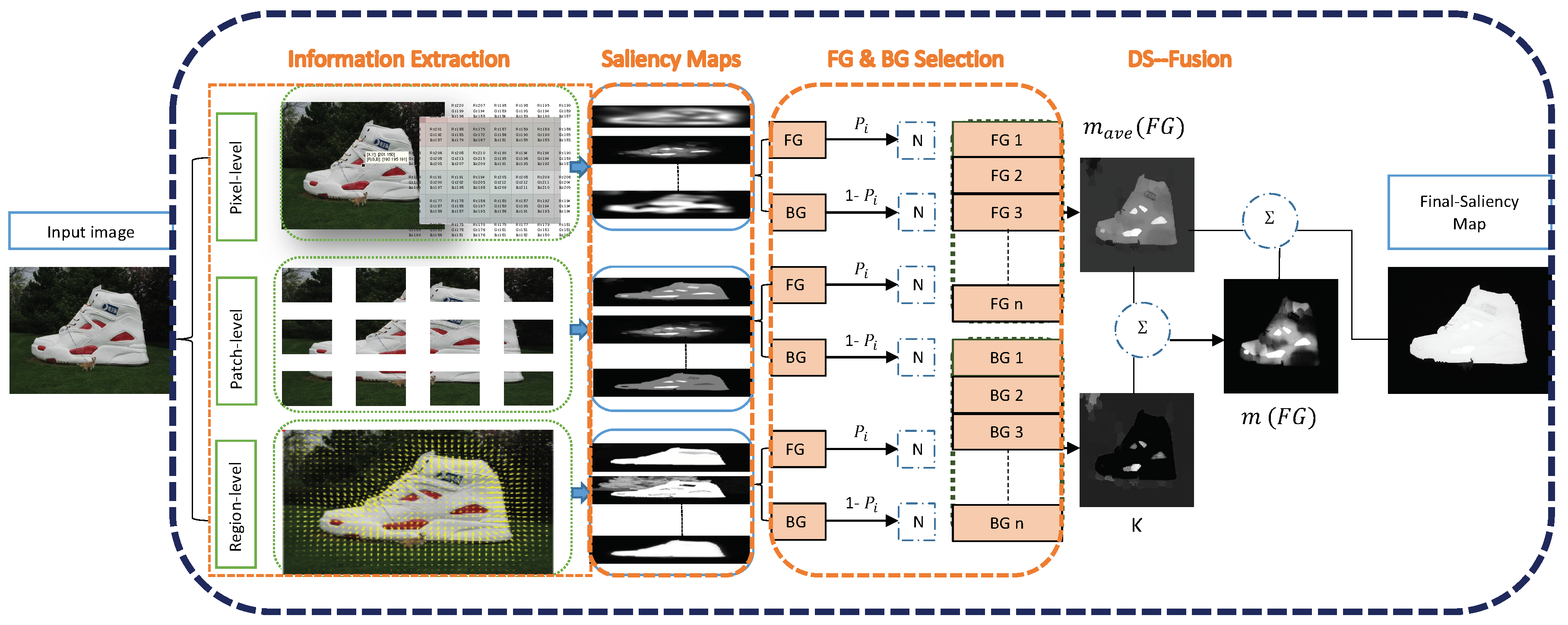
Figure 1. Pipeline of our proposed (DS-OUR) saliency fusion framework (FG denotes the foreground area containing salient pixels, BG represents the background area containing salient pixels and DS-Fusion represents Dempster–Shafer theory of evidence based fusion).
Symmetry 10 00183 g001
Figure 2. Saliency maps comparison, from top left to bottom right: input image (Input), ground truth mask (GT), our saliency map (DS-OUR), and saliency maps of other nine sate of the art approaches DSR [24], GS [13], HS [26], MR [19], MS [27], SF [14], SST [25], XL [20], wCtr [28], respectively.
Symmetry 10 00183 g002
Figure 3. From left to right, (a) Input images; (b) S a l 1 (the weighted mass function generated by Equation (11)); (c) K (addition of foreground and background pixels); (d) S a l 2 (combined saliency map by Equation (13)); (e) S a l ( D S O U R ) final saliency maps by Equation (14); (f) GT (Ground truth mask).
Symmetry 10 00183 g003
Figure 4. Saliency maps comparison, from left to right: first column shows the source input images (Input), ground truth mask (GT), our saliency map (DS-OUR), and saliency maps of other nine state-of-the-art approaches DSR [24], GS [13], HS [26], MR [19], MS [27], SF [14], SST [25], XL [20], wCtr [28], respectively.
Symmetry 10 00183 g004
Figure 5. AUC results on four different datasets, from left to right: DS-OUR, DSR [24], GS [13], HS [26], MR [19], MS [27], SF [14], SST [25], XL [20], wCtr [28], respectively.
Symmetry 10 00183 g005
Figure 6. Qualitative comparison of our method against nine different state-of-the-art algorithms on 4 different datasets, from left to right: First column shows the precision_recall curves, second column shows the ROC curves and third column shows the F-measure results, our method (DS-OUR) performed better than other nine state-of-the-art algorithms.
Symmetry 10 00183 g006
Figure 7. MAE results on four different datasets, from left to right: DS-OUR, DSR [24], GS [13], HS [26], MR [19], MS [27], SF [14], SST [25], XL [20], wCtr [28], respectively.
Symmetry 10 00183 g007
Table 1. Area Under the ROC Curves (AUC), Mean Absolute Error (MAE) and F-measure Comparison Results (AUC/MAE/F-measure).
MethodsMSRAECSSDDUT-OMRONPASCAL-S
DS-OUR0.982/0.061/0.9150.919/0.160/0.7270.901/0.127/0.5720.864/0.195/0.647
DSR0.958/0.096/0.8450.868/0.176/0.6760.862/0.137/0.5180.811/0.205/0.602
GS0.974/0.107/0.8280.879/0.206/0.6090.877/0.174/0.4660.847/0.221/0.596
HS0.966/0.111/0.8660.883/0.228/0.6340.858/0.227/0.5190.833/0.263/0.549
MR0.964/0.075/0.8950.847/0.186/0.6600.845/0.187/0.5280.773/0.229/0.567
MS0.978/0.105/0.8300.913/0.204/0.6710.886/0.210/0.4910.863/0.224/0.601
SF0.899/0.129/0.8080.689/0.219/0.4930.779/0.147/0.4350.646/0.236/0.448
SST0.834/0.223/0.5020.772/0.313/0.3740.799/0.254/0.3200.740/0.302/0.411
XL0.951/0.195/0.7690.837/0.307/0.5020.805/0.332/0.3950.785/0.310/0.465
wCtr0.976/0.066/ 0.8840.881/0.172/0.6770.886/0.144/0.5280.841/0.199/0.629