Ensemble Genetic Fuzzy Neuro Model Applied for the Emergency Medical Service via Unbalanced Data Evaluation


 and
and 
Abstract
1. Introduction
2. Materials and Methods
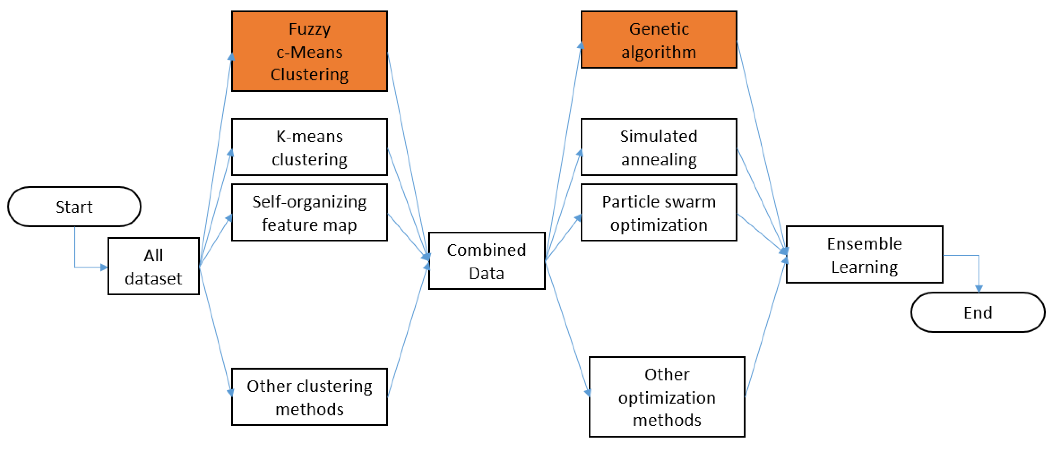
2.1. Fuzzy Clustering
2.2. Artificial Neural Network
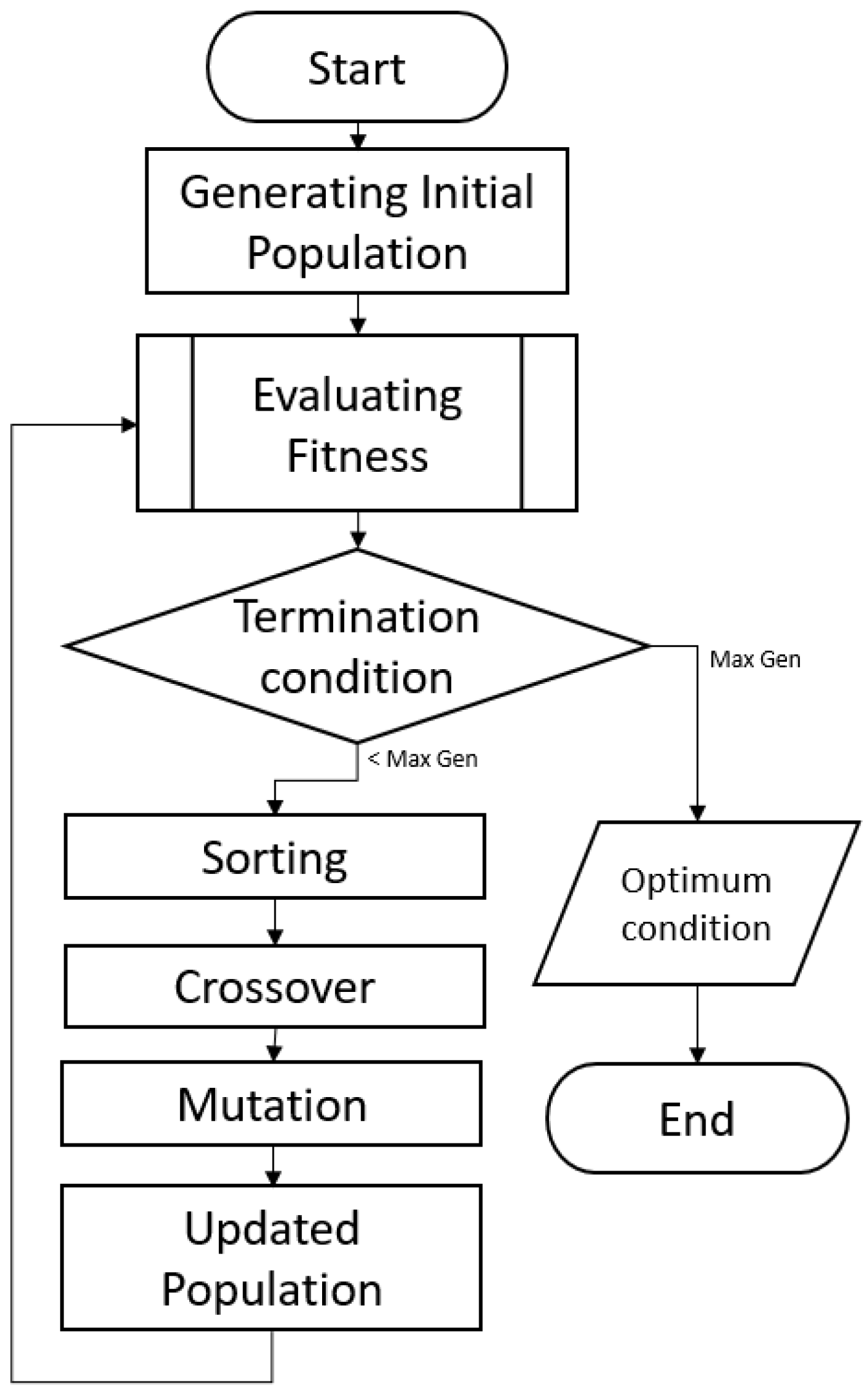
2.3. Genetic Algorithm
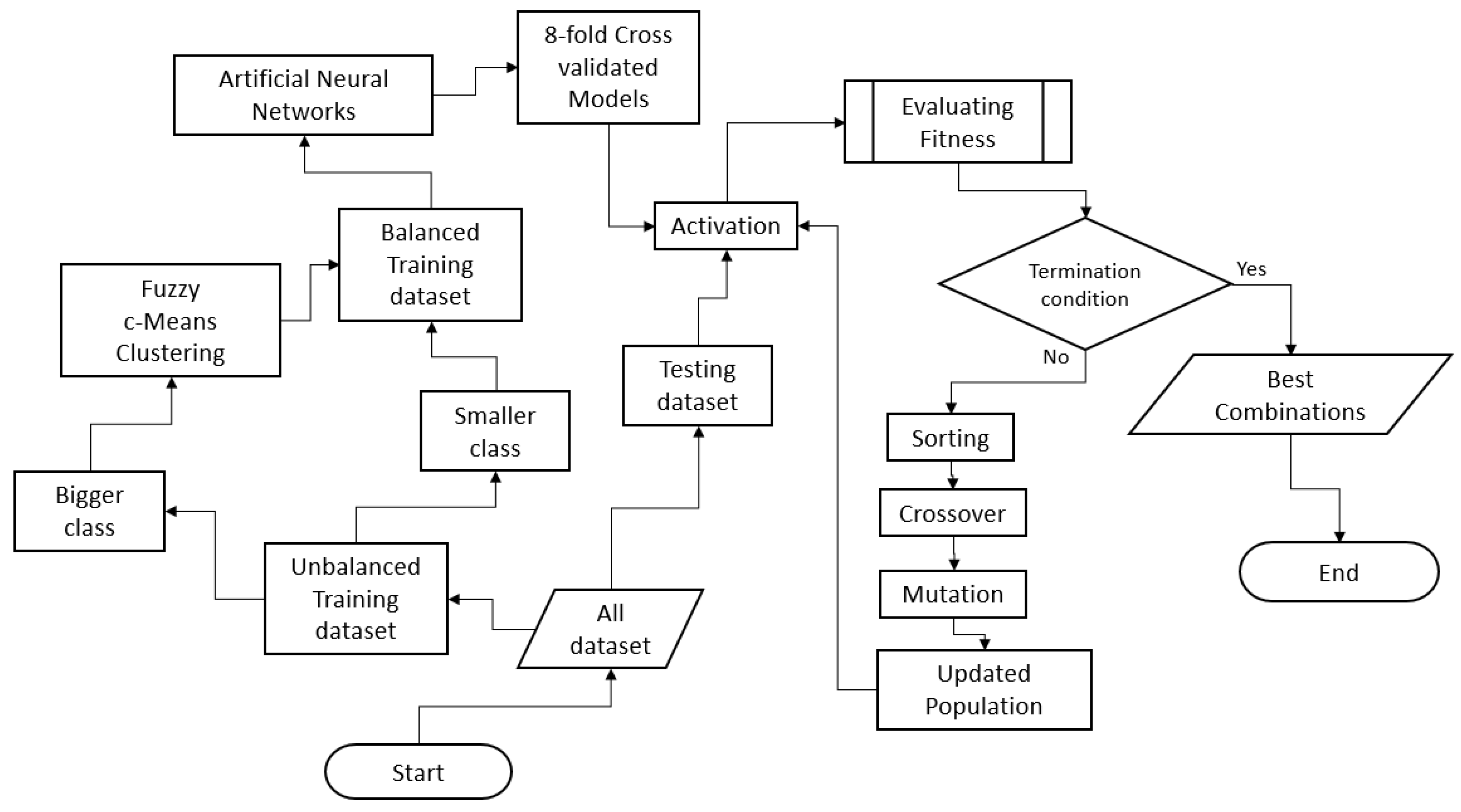
2.4. Ensemble Model
2.5. Performance Evaluation
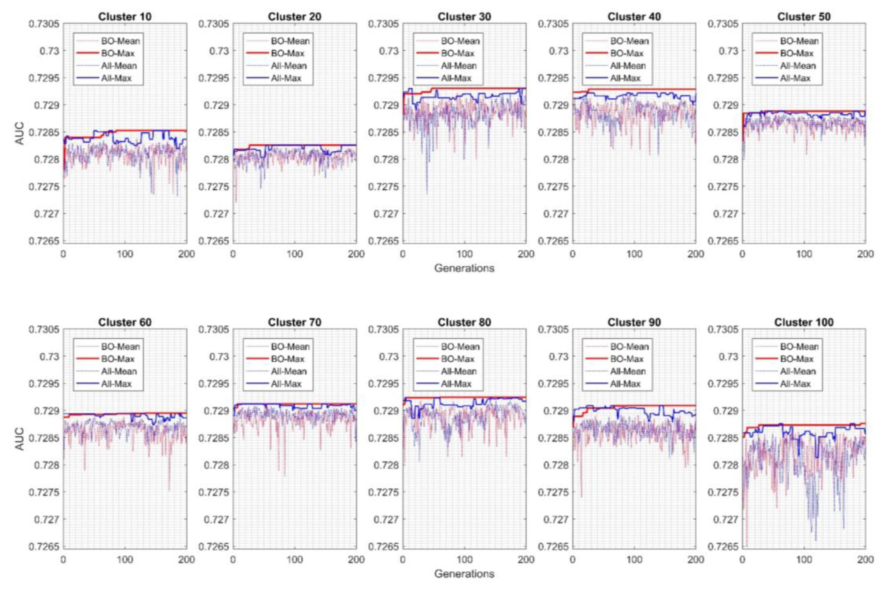
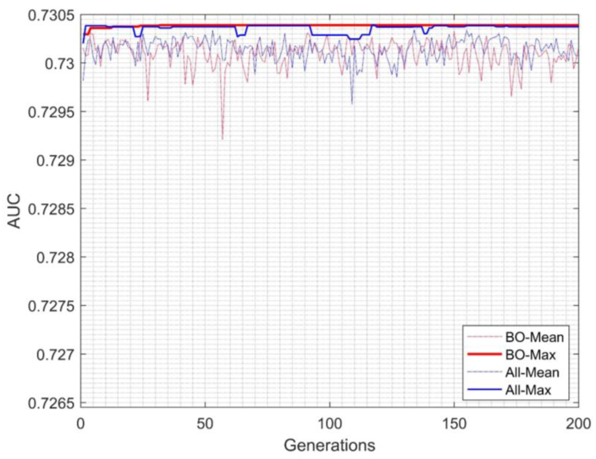
3. Results and Discussion
4. Conclusions and Limitations
Acknowledgments
Author Contributions
Conflicts of Interest
References
- He, H.; Garcia, E.A. Learning from imbalanced data. IEEE Trans. Knowl. Data Eng. 2009, 21, 1263–1284. [Google Scholar]
- Chawla, N.V.; Japkowicz, N.; Kotcz, A. Editorial: Special issue on learning from imbalanced data sets. ACM SIGKDD Explor. Newsl. 2004, 6, 1–6. [Google Scholar] [CrossRef]
- Wang, S.; Yao, X. Multi-class imbalance problems: Analysis and potential solutions. IEEE Trans. Syst. Man Cybern. Part B Cybern. 2012, 42, 1119–1130. [Google Scholar] [CrossRef] [PubMed]
- Provost, F.; Fawcett, T. Robust classification for imprecise environments. Mach. Learn. 2001, 42, 203–231. [Google Scholar] [CrossRef]
- Kubat, M.; Holte, R.C.; Matwin, S. Machine learning for the detection of oil spills in satellite radar images. Mach. Learn. 1998, 30, 195–215. [Google Scholar] [CrossRef]
- Ezawa, K.J.; Singh, M.; Norton, S.W. Learning goal oriented Bayesian networks for telecommunications risk management. In Proceedings of the ICML, Bari, Italy, 3–6 July 1996; pp. 139–147. [Google Scholar]
- Lewis, D.D.; Catlett, J. Heterogeneous uncertainty sampling for supervised learning. In Proceedings of the Eleventh International Conference on Machine Learning, New Brunswick, NJ, USA, 10–13 July 1994; pp. 148–156. [Google Scholar]
- Fawcett, T.; Provost, F. Adaptive fraud detection. Data Min. Knowl. Discov. 1997, 1, 291–316. [Google Scholar] [CrossRef]
- Zhou, B.; Yao, Y.; Luo, J. Cost-sensitive three-way email spam filtering. J. Intell. Inf. Syst. 2014, 42, 19–45. [Google Scholar] [CrossRef]
- Batista, G.E.; Prati, R.C.; Monard, M.C. A study of the behavior of several methods for balancing machine learning training data. ACM SIGKDD Explor. Newsl. 2004, 6, 20–29. [Google Scholar] [CrossRef]
- Cristianini, N.; Shawe-Taylor, J. An Introduction to Support Vector Machines; Cambridge University Press: Cambridge, UK, 2000. [Google Scholar]
- Chawla, N.V.; Bowyer, K.W.; Hall, L.O.; Kegelmeyer, W.P. SMOTE: Synthetic minority over-sampling technique. J. Artif. Intell. Res. 2002, 16, 321–357. [Google Scholar]
- Jain, A.K.; Murty, M.N.; Flynn, P.J. Data clustering: A review. ACM Comput. Surv. CSUR 1999, 31, 264–323. [Google Scholar] [CrossRef]
- Liu, Y.; Hou, T.; Liu, F. Improving fuzzy c-means method for unbalanced dataset. Electron. Lett. 2015, 51, 1880–1882. [Google Scholar] [CrossRef]
- Zhou, B.; Ha, M.; Wang, C. An improved algorithm of unbalanced data SVM. In Fuzzy Information and Engineering; Springer: Berlin/Heidelberg, Germany, 2010; pp. 549–555. [Google Scholar]
- Kocyigit, Y.; Seker, H. Imbalanced data classifier by using ensemble fuzzy c-means clustering. In Proceedings of the 2012 IEEE-EMBS International Conference on Biomedical and Health Informatics (BHI), Hong Kong, China, 5–7 January 2012; pp. 952–955. [Google Scholar]
- Yazdani-Chamzini, A.; Zavadskas, E.K.; Antucheviciene, J.; Bausys, R. A Model for Shovel Capital Cost Estimation, Using a Hybrid Model of Multivariate Regression and Neural Networks. Symmetry 2017, 9, 298. [Google Scholar] [CrossRef]
- Yazdani-Chamzini, A.; Yakhchali, S.H.; Volungevičienė, D.; Zavadskas, E.K. Forecasting gold price changes by using adaptive network fuzzy inference system. J. Bus. Econ. Manag. 2012, 13, 994–1010. [Google Scholar] [CrossRef]
- Geman, S.; Bienenstock, E.; Doursat, R. Neural networks and the bias/variance dilemma. Neural Comput. 1992, 4, 1–58. [Google Scholar] [CrossRef]
- Xie, B.; Liang, Y.; Song, L. Diverse Neural Network Learns True Target Functions. In Proceedings of the 20th International Conference on Artificial Intelligence and Statistics, Fort Lauderdale, FL, USA, 20–22 April 2017; pp. 1216–1224. [Google Scholar]
- Wang, S.; Yao, X. Diversity analysis on imbalanced data sets by using ensemble models. In Proceedings of the IEEE Symposium on Computational Intelligence and Data Mining (CIDM’09), Nashville, TN, USA, 30 March–2 April 2009; pp. 324–331. [Google Scholar]
- Cunningham, P.; Carney, J. Diversity versus quality in classification ensembles based on feature selection. In Proceedings of the European Conference on Machine Learning, Barcelona, Spain, 31 May–2 June 2000; Springer: Berlin/Heidelberg, Germany, 2000; pp. 109–116. [Google Scholar]
- Krogh, A.; Vedelsby, J. Neural network ensembles, cross validation, and active learning. Adv. Neural Inf. Process. Syst. 1995, 7, 231–238. [Google Scholar]
- Brown, G.; Wyatt, J.; Harris, R.; Yao, X. Diversity creation methods: A survey and categorization. Inf. Fusion 2005, 6, 5–20. [Google Scholar] [CrossRef]
- Tumer, K.; Ghosh, J. Theoretical Foundations of Linear and Order Statistics Combiners for Neural Pattern Classifiers. Available online: http://citeseerx.ist.psu.edu/viewdoc/download?doi=10.1.1.36.3954&rep=rep1&type=pdf (accessed on 10 January 2018).
- Xu, L.; Krzyzak, A.; Suen, C.Y. Methods of combining multiple classifiers and their applications to handwriting recognition. IEEE Trans. Syst. Man Cybern. 1992, 22, 418–435. [Google Scholar] [CrossRef]
- Ho, T.K.; Hull, J.J.; Srihari, S.N. Decision combination in multiple classifier systems. IEEE Trans. Pattern Anal. Mach. Intell. 1994, 16, 66–75. [Google Scholar]
- Kittler, J.; Hatef, M.; Duin, R.P.; Matas, J. On combining classifiers. IEEE Trans. Pattern Anal. Mach. Intell. 1998, 20, 226–239. [Google Scholar] [CrossRef]
- Galar, M.; Fernandez, A.; Barrenechea, E.; Bustince, H.; Herrera, F. A review on ensembles for the class imbalance problem: Bagging-, boosting-, and hybrid-based approaches. IEEE Trans. Syst. Man Cybern. Part C Appl. Rev. 2012, 42, 463–484. [Google Scholar] [CrossRef]
- Galar, M.; Fernández, A.; Barrenechea, E.; Herrera, F. EUSBoost: Enhancing ensembles for highly imbalanced data-sets by evolutionary undersampling. Pattern Recognit. 2013, 46, 3460–3471. [Google Scholar] [CrossRef]
- Sanz, J.; Paternain, D.; Galar, M.; Fernandez, J.; Reyero, D.; Belzunegui, T. A new survival status prediction system for severe trauma patients based on a multiple classifier system. Comput. Methods Programs Biomed. 2017, 142, 1–8. [Google Scholar] [CrossRef] [PubMed]
- Zhou, Z.H.; Wu, J.; Tang, W. Ensembling neural networks: Many could be better than all. Artif. Intell. 2002, 137, 239–263. [Google Scholar] [CrossRef]
- Hornby, G.S.; Globus, A.; Linden, D.S.; Lohn, J.D. Automated antenna design with evolutionary algorithms. In Proceedings of the AIAA Space, San Jose, CA, USA, 19–21 September 2006; pp. 19–21. [Google Scholar]
- De Araújo Padilha, C.A.; Barone, D.A.C.; Neto, A.D.D. A multi-level approach using genetic algorithms in an ensemble of Least Squares Support Vector Machines. Knowl. Based Syst. 2016, 106, 85–95. [Google Scholar] [CrossRef]
- Haque, M.N.; Noman, N.; Berretta, R.; Moscato, P. Heterogeneous ensemble combination search using genetic algorithm for class imbalanced data classification. PLoS ONE 2016, 11, e0146116. [Google Scholar] [CrossRef] [PubMed]
- Chen, A.Y.; Lu, T.Y.; Ma, M.H.M.; Sun, W.Z. Demand Forecast Using Data Analytics for the Preallocation of Ambulances. IEEE J. Biomed. Health Inform. 2016, 20, 1178–1187. [Google Scholar] [CrossRef] [PubMed]
- Shieh, J.S.; Yeh, Y.T.; Sun, Y.Z.; Ma, M.H.; Dia, C.Y.; Sadrawi, M.; Abbod, M. Big Data Analysis of Emergency Medical Service Applied to Determine the Survival Rate Effective Factors and Predict the Ambulance Time Variables. In Proceedings of the ISER 50th International Conference, Tokyo, Japan, 29 January 2017. [Google Scholar]
- Ross, T.J. Fuzzy Logic with Engineering Applications; John Wiley & Sons: Hoboken, NJ, USA, 2009. [Google Scholar]
- Bradley, A.P. The use of the area under the ROC curve in the evaluation of machine learning algorithms. Pattern Recognit. 1997, 30, 1145–1159. [Google Scholar] [CrossRef]
- Wong, C.C.; Chen, C.C.; Su, M.C. A novel algorithm for data clustering. Pattern Recognit. 2001, 34, 425–442. [Google Scholar] [CrossRef]
- Jiang, Y.J.; Ma, M.H.M.; Sun, W.Z.; Chang, K.W.; Abbod, M.F.; Shieh, J.S. Ensembled neural networks applied to modeling survival rate for the patients with out-of-hospital cardiac arrest. Artif. Life Robot. 2012, 17, 241–244. [Google Scholar] [CrossRef]
- Qiu, J.; Wei, Y.; Karimi, H.R.; Gao, H. Reliable control of discrete-time piecewise-affine time-delay systems via output feedback. IEEE Trans. Reliab. 2018, 67, 79–91. [Google Scholar] [CrossRef]
- Qiu, J.; Wei, Y.; Wu, L. A novel approach to reliable control of piecewise affine systems with actuator faults. IEEE Trans. Circuits Syst. II Express Briefs 2017, 64, 957–961. [Google Scholar] [CrossRef]


| Prediction | |||
|---|---|---|---|
| Positive | Negative | ||
| Reference | Positive | True Positive (TP) | False Negative (FN) |
| Negative | False Positive (FP) | True Negative (TN) | |
| Best Comb. | Age | Gender | Reaction Time | On-Scene Time | Transportation Time | Frequency |
|---|---|---|---|---|---|---|
| 1 | Middle-Age | Male | Very Short | Very Short | Very Short | 65,039 |
| 2 | Adult | Male | Very Short | Very Short | Very Short | 62,790 |
| 3 | Adult | Female | Very Short | Very Short | Very Short | 57,455 |
| 4 | Middle-Old | Male | Very Short | Very Short | Very Short | 50,839 |
| 5 | Middle-Age | Female | Very Short | Very Short | Very Short | 49,665 |
| 6 | Young | Male | Very Short | Very Short | Very Short | 39,142 |
| 7 | Middle-Old | Female | Very Short | Very Short | Very Short | 37,615 |
| 8 | Young | Female | Very Short | Very Short | Very Short | 29,567 |
| 9 | Middle-Age | Male | Very Short | Short | Very Short | 29,344 |
| 10 | Adult | Male | Very Short | Short | Very Short | 27,876 |
| Cluster | Fold | Min | Max | Mean | SD | |||||||
|---|---|---|---|---|---|---|---|---|---|---|---|---|
| 1 | 2 | 3 | 4 | 5 | 6 | 7 | 8 | |||||
| 10 | 0.7273 | 0.7270 | 0.7263 | 0.7253 | 0.7253 | 0.7251 | 0.7246 | 0.7243 | 0.7243 | 0.7273 | 0.7256 | 0.0011 |
| 20 | 0.7258 | 0.7251 | 0.7275 | 0.7275 | 0.7266 | 0.7256 | 0.7262 | 0.7246 | 0.7246 | 0.7275 | 0.7261 | 0.0010 |
| 30 | 0.7266 | 0.7259 | 0.7267 | 0.7276 | 0.7269 | 0.7271 | 0.7273 | 0.7257 | 0.7257 | 0.7276 | 0.7267 | 0.0006 |
| 40 | 0.7281 | 0.7265 | 0.7265 | 0.7271 | 0.7268 | 0.7275 | 0.7254 | 0.7273 | 0.7254 | 0.7281 | 0.7269 | 0.0008 |
| 50 | 0.7261 | 0.7270 | 0.7275 | 0.7261 | 0.7265 | 0.7262 | 0.7253 | 0.7255 | 0.7253 | 0.7275 | 0.7263 | 0.0007 |
| 60 | 0.7249 | 0.7265 | 0.7267 | 0.7277 | 0.7278 | 0.7275 | 0.7271 | 0.7250 | 0.7249 | 0.7278 | 0.7266 | 0.0011 |
| 70 | 0.7248 | 0.7270 | 0.7261 | 0.7263 | 0.7267 | 0.7254 | 0.7250 | 0.7252 | 0.7248 | 0.7270 | 0.7258 | 0.0008 |
| 80 | 0.7264 | 0.7267 | 0.7268 | 0.7270 | 0.7277 | 0.7246 | 0.7257 | 0.7253 | 0.7246 | 0.7277 | 0.7263 | 0.0010 |
| 90 | 0.7267 | 0.7265 | 0.7276 | 0.7275 | 0.7257 | 0.7265 | 0.7265 | 0.7237 | 0.7237 | 0.7276 | 0.7263 | 0.0012 |
| 100 | 0.7251 | 0.7208 | 0.7256 | 0.7236 | 0.7255 | 0.7254 | 0.7259 | 0.7234 | 0.7208 | 0.7259 | 0.7244 | 0.0017 |
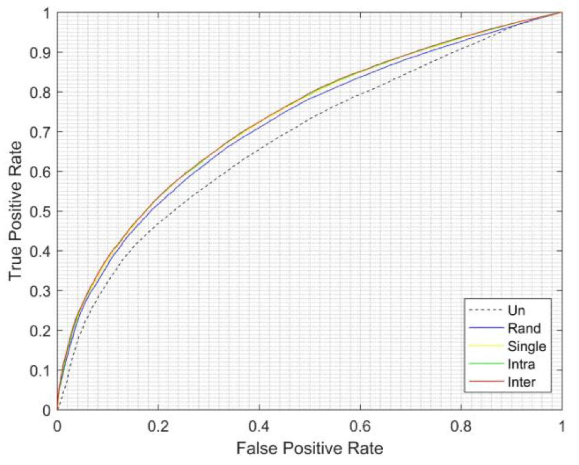
| Cluster | Unbalanced | Random | Single | Intra-Cluster EGFNM |
|---|---|---|---|---|
| 10 | 0.67974 | 0.7177 | 0.727263 | 0.7285 |
| 20 | 0.727483 | 0.7283 | ||
| 30 | 0.727619 | 0.7293 | ||
| 40 | 0.728061 | 0.72928 | ||
| 50 | 0.727472 | 0.7289 | ||
| 60 | 0.72779 | 0.7289 | ||
| 70 | 0.727002 | 0.7291 | ||
| 80 | 0.7277 | 0.7292 | ||
| 90 | 0.727603 | 0.7291 | ||
| 100 | 0.72593 | 0.7288 |
| Cluster | Hidden Neuron on Layer | ||
|---|---|---|---|
| 1 | 2 | 3 | |
| 30 | 7 | 13 | 28 |
| 40 | 30 | 27 | 18 |
| 50 | 19 | 11 | 47 |
| 60 | 19 | 49 | 26 |
| 70 | 21 | 32 | 32 |
| 80 | 5 | 42 | 37 |
| 90 | 8 | 41 | 46 |
| 100 | 18 | 37 | 9 |
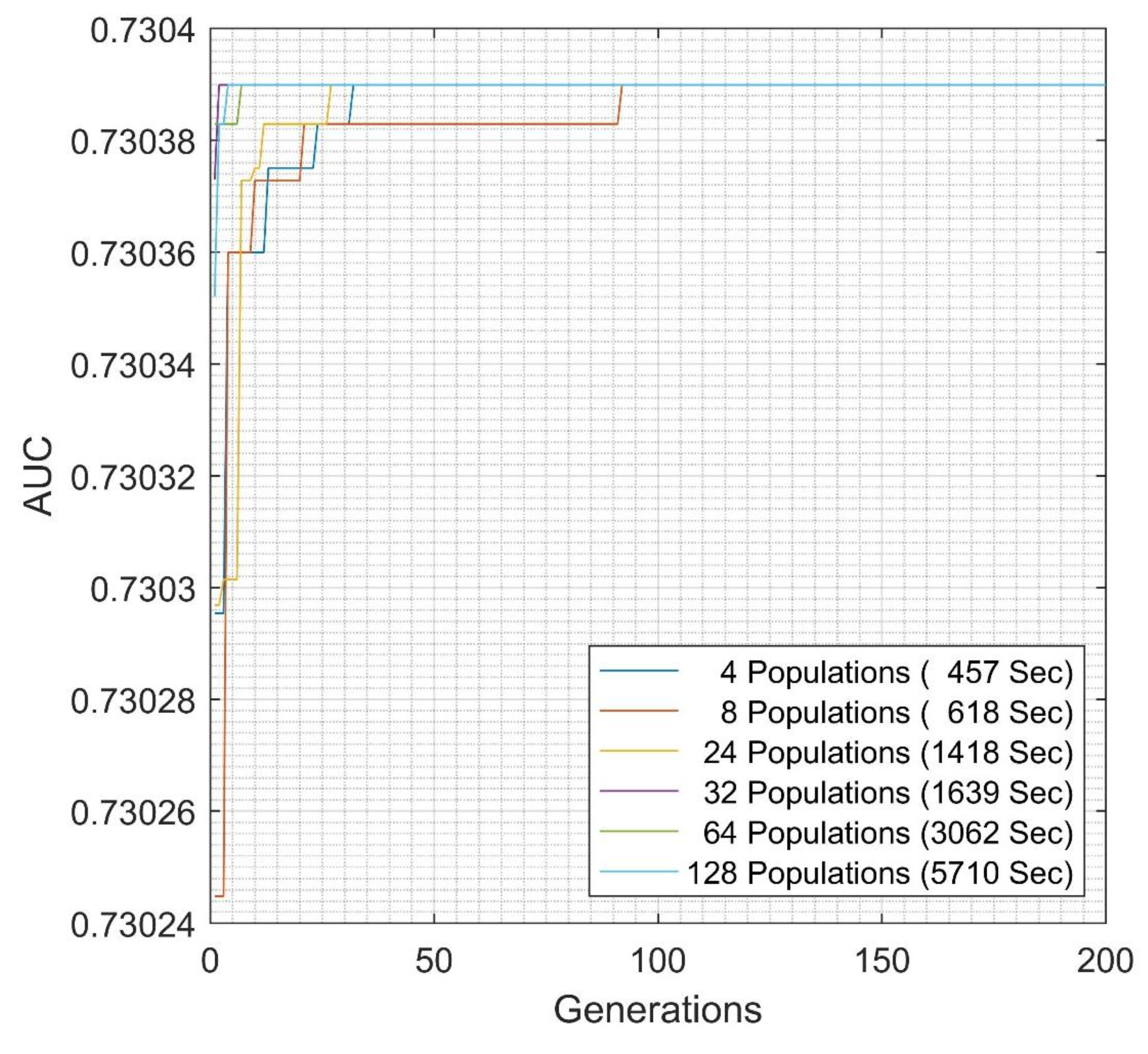
| Methods | Cluster | Maximum AUC | EGFNM Generation |
|---|---|---|---|
| Intra-cluster EGFNM | 10 | 0.7285 | 89 |
| 20 | 0.7283 | 30 | |
| 30 | 0.7293 | 50 | |
| 40 | 0.72928 | 29 | |
| 50 | 0.7289 | 39 | |
| 60 | 0.7289 | 136 | |
| 70 | 0.7291 | 11 | |
| 80 | 0.7292 | 63 | |
| 90 | 0.7291 | 70 | |
| 100 | 0.7288 | 195 | |
| Inter-cluster EGFNM | Ensemble | 0.73038 | 27 |
© 2018 by the authors. Licensee MDPI, Basel, Switzerland. This article is an open access article distributed under the terms and conditions of the Creative Commons Attribution (CC BY) license (http://creativecommons.org/licenses/by/4.0/).
Share and Cite
Sadrawi, M.; Sun, W.-Z.; Ma, M.H.-M.; Yeh, Y.-T.; Abbod, M.F.; Shieh, J.-S. Ensemble Genetic Fuzzy Neuro Model Applied for the Emergency Medical Service via Unbalanced Data Evaluation. Symmetry 2018, 10, 71. https://doi.org/10.3390/sym10030071
Sadrawi M, Sun W-Z, Ma MH-M, Yeh Y-T, Abbod MF, Shieh J-S. Ensemble Genetic Fuzzy Neuro Model Applied for the Emergency Medical Service via Unbalanced Data Evaluation. Symmetry. 2018; 10(3):71. https://doi.org/10.3390/sym10030071
Chicago/Turabian StyleSadrawi, Muammar, Wei-Zen Sun, Matthew Huei-Ming Ma, Yu-Ting Yeh, Maysam F. Abbod, and Jiann-Shing Shieh. 2018. "Ensemble Genetic Fuzzy Neuro Model Applied for the Emergency Medical Service via Unbalanced Data Evaluation" Symmetry 10, no. 3: 71. https://doi.org/10.3390/sym10030071
APA StyleSadrawi, M., Sun, W.-Z., Ma, M. H.-M., Yeh, Y.-T., Abbod, M. F., & Shieh, J.-S. (2018). Ensemble Genetic Fuzzy Neuro Model Applied for the Emergency Medical Service via Unbalanced Data Evaluation. Symmetry, 10(3), 71. https://doi.org/10.3390/sym10030071