A Novel Adaptive Non-Local Means-Based Nonlinear Fitting for Visibility Improving

Abstract

The spatial-based method has become the most widely used method in improving the visibility of images. The visibility improving is mainly to remove the noise in the image, in order to trade off denoising and detail maintaining. A novel adaptive non-local means-based nonlinear fitting method is proposed in this paper. Firstly, according to the smoothness of the intensity around the central pixel, eight kinds of templates with different precision are exploited to approximate the central pixel through a novel adaptive non-local means filter design; the approximate weight coefficients of templates are derived from the approximation credibility. Subsequently, the fractal correction is used to smooth the denoising results. Eventually, the Rockafellar multiplier method is employed to generalize the smooth plane fitting to any geometric surface, thus yielding the optimal fitting of the center pixel approximation. Through a large number of experiments, it is clearly elucidated that compared with the classical spatial iteration-based methods and the recent denoising algorithms, the proposed algorithm is more robust and has better effect on denoising, while keeping more original details during denoising.

1. Introduction

Digital images are obtained by digitizing analog images, which can be stored and processed by computer. With the development of science and technology, digital images have been widely recognized and applied. However, there is always noise in the obtained images, which has a negative impact on conveying real information. Thus, researchers urgently need to reduce the noise to a minimum. Image noise-reduction, noise-suppression and noise-removal are widely used processing technologies for images. By using these technologies, we can obtain the expected images and improve the peak signal to noise ratio of images (SNR).

In recent years, there have been many related researches on denoising. In view of the research direction, there are two main kinds of denoising thoughts. One is to use directly mathematical operations and filtering methods to process images in the spatial domain. The other is to process the images in a certain transform domain. The classical methods of denoising in the spatial domain mainly include the threshold method, field average method, median filter, wiener filter and so on [1]. On the basis of these researches, the direction of the improvements is mainly to simplify the operation and improve the processing effects. Related researches mainly include: Chenglin Zuo et al. [2] proposed an image denoising method using quadtree-based nonlocal means with locally adaptive principal component analysis, and the proposed method achieves spatially uniform denoising. Jian Sun et al. [3] proposed a novel approach for color image denoising via discriminatively learned iterative shrinkage, which can achieve good denoising result for color images. Sujit Kumar Sahoo et al. [4] analyzed the process of introducing noise, definitely derived the noise components in a dictionary update step, and proposed a superior solution for the desired SNR. Meng Li et al. [5] proposed a denoising algorithm based on a fast translation invariant (FTI) algorithm and a more general K-translation invariant (K-TI) algorithm. The algorithm has the appealing performance for general multidimensional images with Poisson or Gaussian noise. Y. Zhan et al. [6] proposed an image denoising method based on machine learning by using high order singular value decomposition (HOSVD). The method has an ideal denoising effect on gray images and color images. Y. Zhan et al. [7] proposed a controlled denoising method for non-local means image, which can adaptively tune the decay parameter for each image pixel. Xiangchu Feng et al. [8] proposed a two-directional nonlocal variational model (TDNL) to reduce noise according to the principle of internal similarity. Karen Panetta et al. [9] proposed a sequence-to-sequence similarity-based filter for image denoising. Lianghai et al. [10] proposed a two-stage quaternion switching vector filter for color impulse noise removal. Ahmed Ben Said et al. [11] proposed a Multispectral image denoising with optimized vector non-local mean filter to illustrate the efficiency of the approach in terms of both denoising performance and computation complexity. Jonatas Lopes de Paivaa et al. [12] proposed an approach based on hybrid genetic algorithm (HGA) applied to the image denoising problem. DengLiang Jian et al. [13] proposed a fast image recovery algorithm based on splitting deblurring and denoising. Yun Zhanga et al. [14] proposed a new fuzzy density weight SVR (FDW-SVR) denoising algorithm, which assigns fuzzy priority to each sample according to its density weight. Xiong Xiangtuan et al. [15] proposed several variations of the Gaussian model, which are derived from the varied diffusion variations for image denoising. Gouchol Pok et al. [16] proposed an efficient block-based image-denoising method, which is devised specially for fast denoising of impulse noise. Bo Du et al. [17] proposed a bandwise noise model to denoise. Furthermore, based on the low-rank structure of the HSI, the proposed bandwise noise model is combined with the low-rank matrix factorization to obtain a new efficient HSI denoising algorithm. Yuzhen Niu et al. [18] proposed a region-aware image denoising algorithm (RAID) by exploring parameter preference. Qingsong Yang et al. [19] introduced a new CT image denoising method based on the generative adversarial network (GAN) with Wasserstein distance and perceptual similarity. Saeed Anwar et al. [20] present a novel image denoising algorithm that uses an external, category-specific image database within the spatial locality of each noisy patch.

Fourier transform and wavelet are classical methods in the transform domain to reduce noise. There are mainly three kinds of improvement directions, including denoising combined with correlation, denoising combined with singularity detection and denoising based on the coefficient threshold in the wavelet domain. Related researches mainly include: Sethunadh R.S et al. [21] proposed a spatial adaptive denoising method based on directionlet transform to reduce Gaussian noise by considering the correlation of the directionlet coefficients across different scales. Norbert Remenyi et al. [22] proposed an image denoising method based on 2D scale-mixing complex wavelet transforms which uses empirical Bayesian method to achieve good effect. Fumitaka Hosotani et al. [23] proposed a zero-mean white Gaussian noise removal method via a high-resolution frequency analysis. Jingjing Dai et al. [24] proposed a novel color image denoising called multichannel nonlocal means fusion (MNLF) to improve the performance for various noises by denoising as a minimized threshold function. Mina Sharifymoghaddam et al. [25] proposed a pre-processing hard thresholding algorithm that eliminates those dissimilar patches to improve the performance of denoising. Jinn Ho et al. [26] proposed a denoising method by using hidden Bayesian network constructed from a wavelet coefficient to build a model for prior probability of the original image. Then, the method uses the belief propagation (BP) algorithm as the maximum-a-posterior estimator to derive denoised wavelet coefficients. Jose Manuel Mejia et al. [27] presented an algorithm for the denoising of small animal positron emission images. The proposed algorithm combines a multiresolution transform with robust filtering of regions. Zhaoming Kong et al. [28] considered characterizing MR images with 3-D operators, and presented a novel 4-D transform-domain method termed `modified nonlocal tensor-SVD’ for MR image denoising. Urvashi Prakash Shukla [29] proposed a novel denoising method based on the concept of Hilbert vibration decomposition (HVD). Xiao Bai et al. [30] proposed a novel hyperspectral image denoising method based on tucker decomposition to model the nonlocal similarity across the spatial domain and the global similarity along the spectral domain. Gulsher Baloch et al. [31] proposed a new residual correlation-based regularization for image denoising. The regularization can effectively render residual patches as uncorrelated as possible.

By analyzing the research achievements above, we find that the improved methods have ideal effects and practical application value. Besides, the process is often greatly simplified. However, these methods usually neglect the target geometry information, it makes the edge information of the processing results incomplete and the interested information reduced for future research.

This paper aims at a prominent problem in the existing denoising algorithms, a new image denoising algorithm based on non-local means theory in spatial domain is proposed. For the edge information, the method gives full consideration to geometric information of the target image, an eight asymmetric spatial templates approximate method is designed and nonlinear algebraic optimization is used to fit the optimal solution to the approximate center pixel. The rest of the work is organized as follows. In the second part, we will introduce the evolutionary process of the algorithm. The third part will focus on the proposed algorithm in this paper. The fourth part will focus on the analysis of the experiment. We will compare the proposed method with the existing denoising algorithms to obtain the application value and processing advantages of the proposed method. The fifth part will be the summary of the full text.

2. The Feasibility Analysis of Adaptive Geometric Non-Local Means Denosing Theory

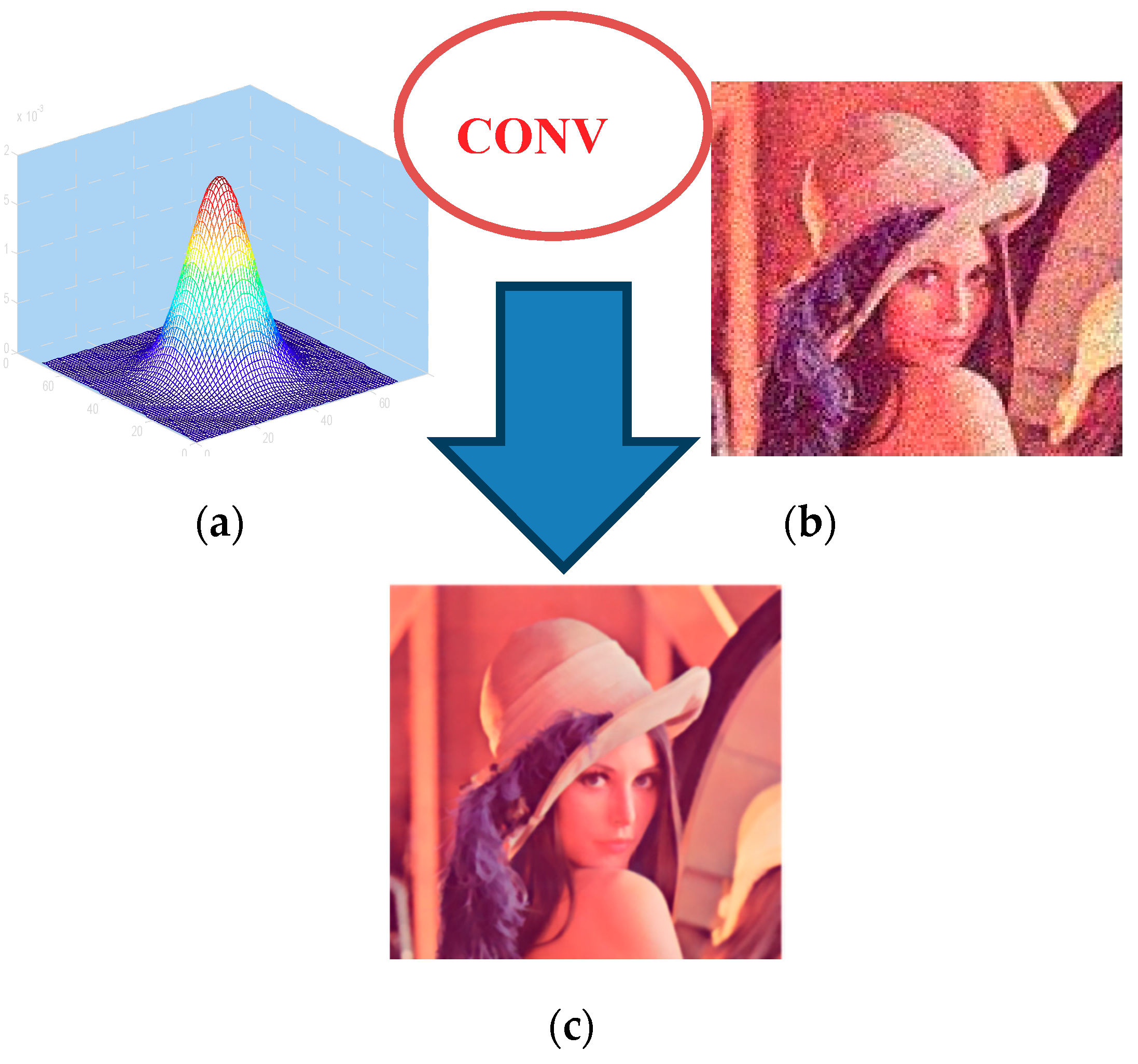
Among traditional spatial filtering methods, linear filtering is the most classical. As shown in Figure 1, we briefly introduce the typical Gauss convolution filtering process and convolution operation with the $n\times n$ Gauss kernel in Figure 1a and the original image in Figure 1b to get the filtered image in Figure 1c.

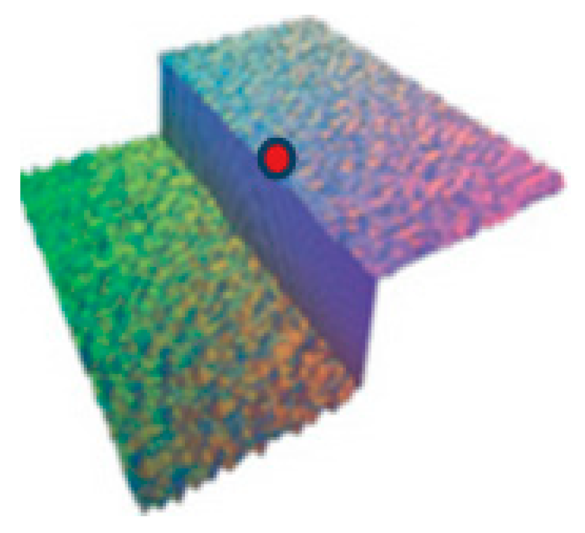
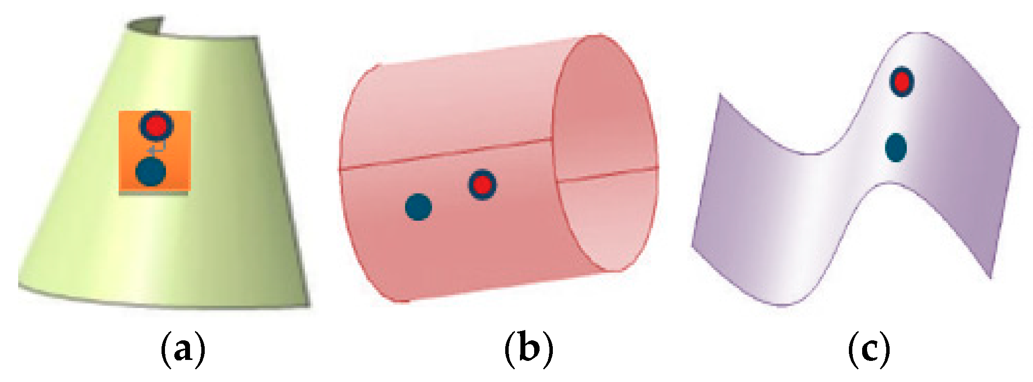
However, the traditional filtering has neglected the target in the image which often contains the geometric shape information. It can be described as plane, inclined plane or curved surface. For the plane and the inclined plane, the gray value of the pixel is a linear change; we can use the gray information points surrounding the center point to replace the gray value of it. For curved surface, we found that it can be divided into three categories: conical surface, cylindrical surface and extruded surface. As shown in Figure 2, in a small neighborhood, the red points are on the tangent plane of the blue point. In other word, in a small neighborhood of the curved surface, the center point can still be represented by the surrounding neighborhood points [32,33].

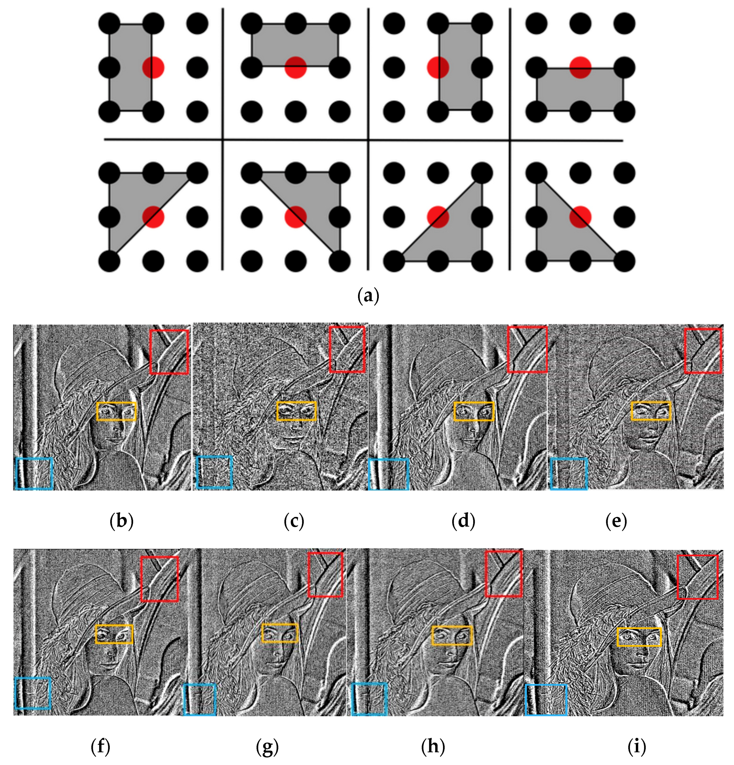
Thus, for the continuous surface, we can use the gray value of the surrounding points to replace the center point, no matter if it is a plane, an inclined plane or a curved surface. For the fracture surface, the approximation of the central point cannot be directly replaced by the surrounding points. As shown in Figure 3, when the red center point is at the edge and the red center point with surrounding points is on the same plane, the center points can be expressed by the gray value of the neighboring points. If the center point is in the edge of the section, it is not reasonable to simply weight surrounding points to express this point. Thus, this paper proposes to fit the optimal approximate solution of any plane in the light of uncertainty of the center point. In this section, in order to demonstrate the feasibility of geometric fractal approximation, we design asymmetric approximation templates as a spatial filter to denoise. We divide the random plane into eight different forms, in each of which exists the best approximation of a red center pixel.

The experimental results show that the approximation result of each pixel in the image is better than the approximation of the whole image in primary vision. It can be expressed as follow: (1) In the space domain of the image, we mainly use the convolution between functions to obtain the global approximation. In this way, the critical value of the function is often neglected or similar, which definitely leads to the final result losing some detailed information; (2) in the image transform domain, the information of the original image will be changed in the process of regional transformation due to the range of the function. However, this local mean denoising method still has the following problems: (1) Mean approximation plays more of a role in image smoothing; however, the local image information will become blurred. The different approximation of templates selection will produce different results (Information of Figure 4 in box); (2) when the noise is random, the application range of the algorithm is limited by a certain approximation. Its adaptive denoising ability is limited; (3) it does not make full use of the information of different neighborhoods in the image. The simple local mean will often lead to the image being over smooth or not smooth enough. In addition, the edge information of the restored image is not clear; (4) for the region where the gray value has a sudden change in the image, that is, the non-local mean will lead to producing information distortion. New noise points may appear. In order to solve the above problems, this paper puts forward a novel adaptive non-local means denoising algorithm.

3. Design of Spatial Geometric Fractal Iterative Denoising Algorithm

In Figure 4, each center point has eight kinds of geometric forms. In the image filtering process, eight kinds of geometric approximation will produce eight results. In another way, the gray value of each center $f(s)$ (the red point in the figure) can produce eight approximation $g_i(x) i=1,2,\dots ,8$. Thus, we need to represent the gray value of the red point by the eight geometric approximation results [34,35].

$$\widehat{f}(x)=F(g_i(x))\begin{array}{cc}& i=1,2\dots ,8\end{array}$$

(1)

where $\widehat{f}(x)$ is the estimated result of x, F is assumed as an estimation arithmetic and $g_i(x)$ denotes one of the estimated results.

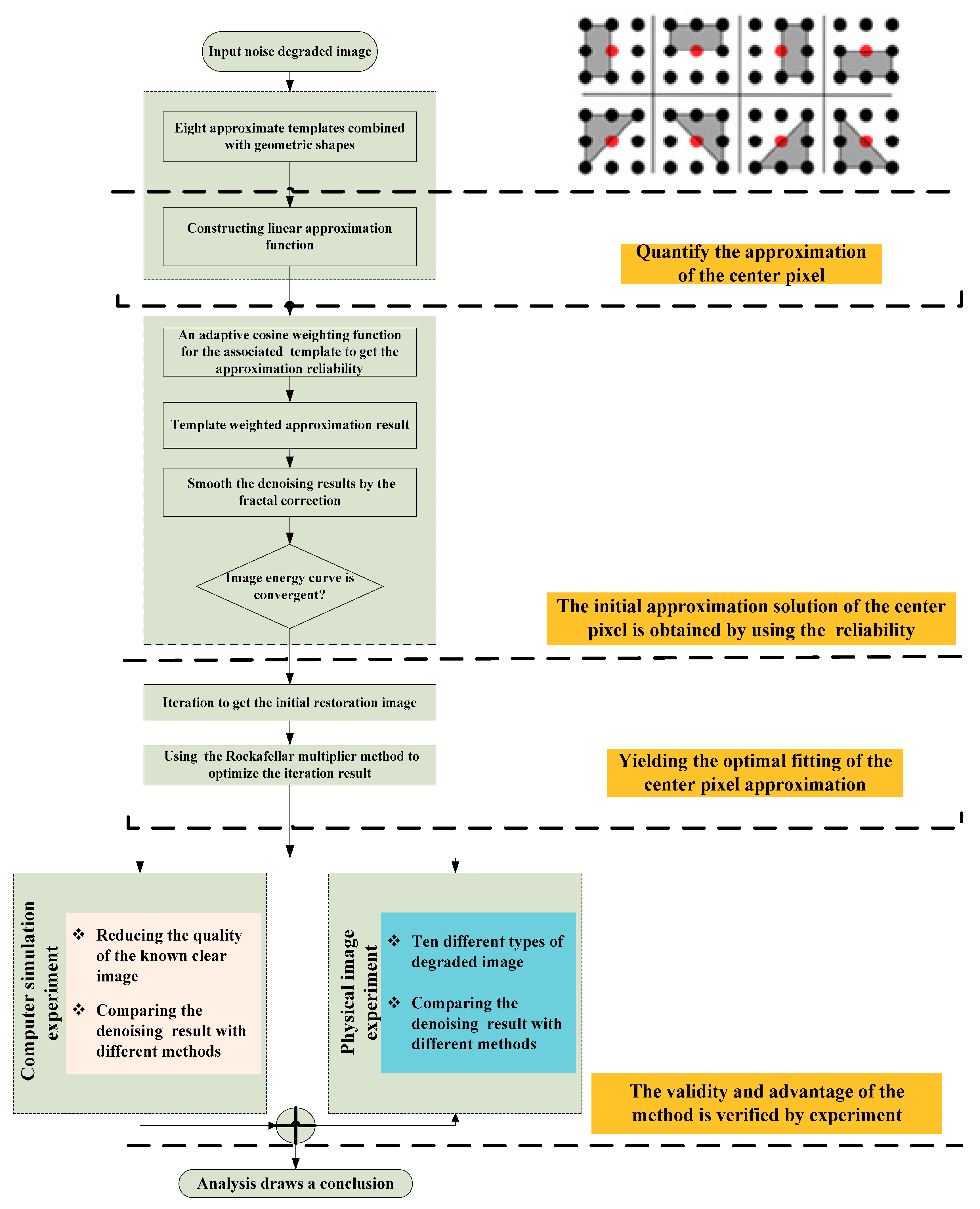
In this paper, on the basis of the idea of non-local mean approximation, we design an adaptive approximation kernel function and use fractal theory for smoothing. This method makes full use of different neighborhood information of the noise image; the adaptive denoising performance is guaranteed under different noise scales. Meanwhile, in the fitting process, eight asymmetric spatial filtering templates and nonlinear algebraic optimization are used to give full consideration of the subject’s information and edge section information to retain the details of original image. In addition, we use graph theory to optimize the preliminary approximation results to ensure that the information in the case of mutation still gets the desired denoising effect.

The software process in this paper is shown in Figure 5.

3.1. Adaptive Geometry Non-Local Means Denoising Model

In terms of probability, if the approximation result is closer to the actual value, the weight is greater; if the approximation result is not suitable for the actual value, the weight is relatively small. Equation (1) can be converted to Equation (2).

$$\widehat{f}(x)={\displaystyle \sum _{i=1}^8{w}_i{g}_i(x)},{\displaystyle \sum w_i=1}$$

(2)

where, $w_i$ is the corresponding weight of the ith template. Equation (2) represents that the ultimate replacement value of the red point is the result of the linear combination of eight approximation values. Within a certain range of noise, we can use the eight types of approximation methods for images with different SNR. The smaller the difference between the result and the clear image is, the greater the probability that the estimation point and center point are in the continuous surface. On the contrary, when the difference is large, the probability that the gray value between the estimation point and the center point may exist cross section, and the estimated result is not reliable.

$$w_i=f_{k,i}(\Delta )$$

(3)

where $\Delta$ is the difference between the estimated value and the center point, $f_{k,i}()$ is the relation between the difference and the weight. Finding an appropriate mapping relationship can accurately determine the weight $w_i$.

Thus, determining the weights of the non-local weighted mean filter has two key issues. One of them is that we must obtain the similarity between the central pixel and the eight different approximation methods. The other issue is the design of the approximation kernel function.

3.1.1. New Similarity Description Method

According to the row priority principle, the gray level matrix is expanded to build two sets of six-dimensional gray vectors. One of set is ${\mathbb{Z}}_a$, which consists of a central pixel value in the image, and the other is ${\mathbb{Z}}_1$~${\mathbb{Z}}_8$ consisting of eight approximating templates. According to the theory of non-local mean denoising, when the center pixels are approximated by different templates, the error is caused by the difference of similarity. Usually, the similarity of vectors can be obtained by the Euler distance. However, this method may lead to the following problems: (1) Two kinds of vectors are composed of image pixels, they not only have numerical information but also have the content of the image information, such as boundary information. If we only consider the numerical similarity of the vector, it will cause the distortion of the image content information, and it will be possible to bring the artificial features such as ring or pixel-ladder; (2) when the image has strong noise, the Euclidean distance cannot reflect ideally the similarity between the vectors.

In order to solve the above two problems, this paper introduces the principle of cosine distance and gray region similarity to modify the weight of the non-local mean method. The weighted distance Equation of regional similarity $\mathrm{\Omega }(i,j)$ can be obtained by Equation (4):

$$\mathrm{\Omega }(i,j)=\frac{{\omega }_c(a,k){\omega }_s(a,k){\Vert g\left({\mathbb{Z}}_a\right)-g\left({\mathbb{Z}}_k\right)\Vert }_{2,\lambda }}{8\cos <{\mathbb{Z}}_a,{\mathbb{Z}}_k>}, k\in [1,8]$$

(4)

where, ${\omega }_c(a,k)$ is the similarity weight for ${\mathbb{Z}}_1$~${\mathbb{Z}}_8$ and ${\mathbb{Z}}_a$, which is shown in Equation (5). ${\Vert g\left({\mathbb{Z}}_a\right)-g\left({\mathbb{Z}}_k\right)\Vert }_{2,\lambda }$ is the Euclidean distance between ${\mathbb{Z}}_1$~${\mathbb{Z}}_8$ and ${\mathbb{Z}}_a$, and $\lambda$ is the standard deviation of Gauss kernel. $\cos <{\mathbb{Z}}_a,{\mathbb{Z}}_k>$ represents cosine distance between ${\mathbb{Z}}_1$~${\mathbb{Z}}_8$ and ${\mathbb{Z}}_a$.

$${\omega }_c(a,k)=\frac{1-corr}{2},k\in [1,8]$$

(5)

where, corr is the correlation coefficient between ${\mathbb{Z}}_1$~${\mathbb{Z}}_8$ and ${\mathbb{Z}}_a$, it is between 0 and 1, ${\omega }_s(a,k)$ is the distance weight for ${\mathbb{Z}}_1$~${\mathbb{Z}}_8$ and ${\mathbb{Z}}_a$.

$${\omega }_s(a,k)=\frac{1}{2}\Vert \mathrm{I}\left(a\right)-\mathrm{I}\left(k\right)\Vert , k\in [1,8]$$

(6)

where, $\Vert \mathrm{I}\left(a\right)-\mathrm{I}\left(k\right)\Vert$ is the coordinate distance between the center pixel and the gravity pixel of the eight kinds of approximation templates.

3.1.2. New Adaptive Association Approximation Kernel Function

Original Non-local Means (ONLM) uses the exponential kernel function:

$$f_k=\exp \left(-\frac{\mathrm{D}(a,k)}{{\sigma }^2}\right), k\in [1,8]$$

(7)

where, $\sigma$ is the attenuation factor of the exponential function, it also affects the denoising performance of the algorithm; $\mathrm{D}(a,k)$ is the Euclidean distance between the center and neighborhood pixel.

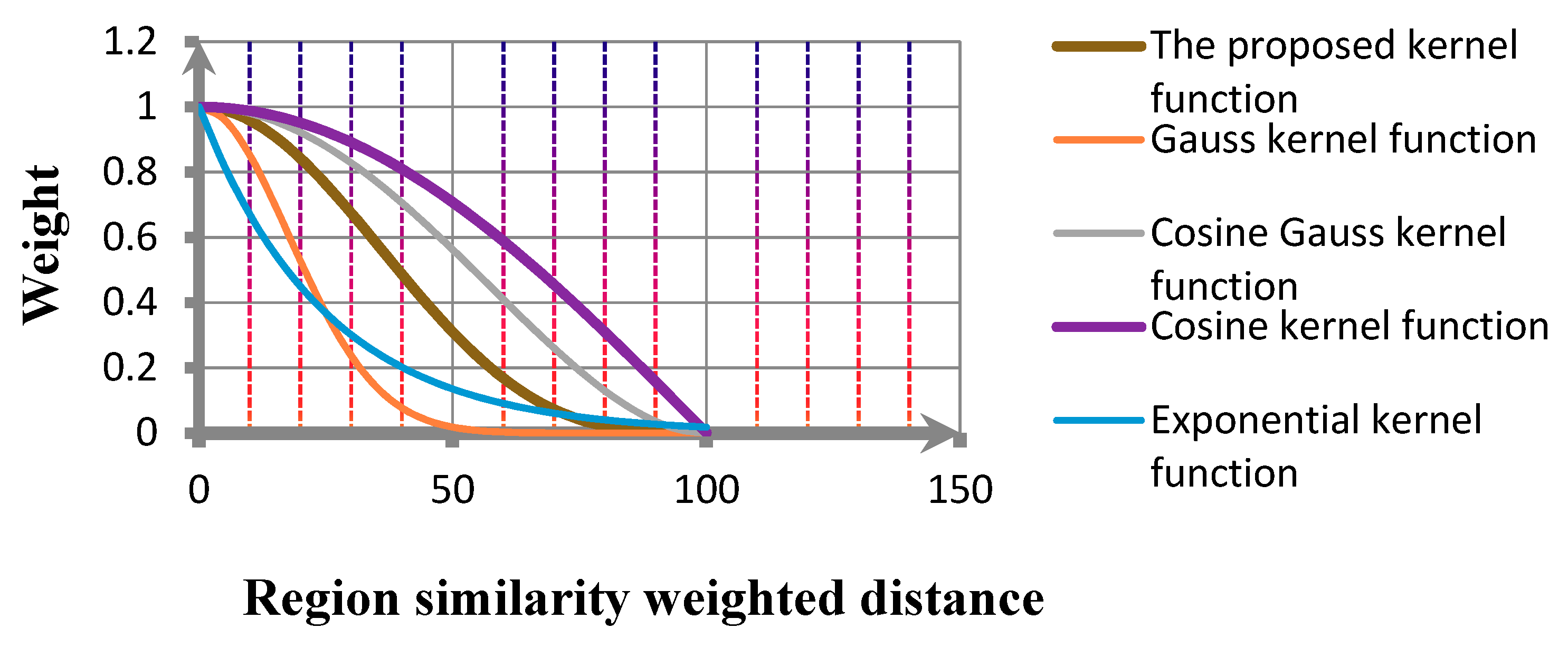
Combining the analysis of different kernel functions, we propose a novel adaptive association approximation kernel function by the analysis of the actual data, as shown in Equation (8).

$$f_k(x)=\{\begin{array}{l}\exp \left(-\frac{{\mathrm{\Omega }}^2(i,j)}{{\sigma }^2}\right)\cos \left(\frac{\pi }{2}\frac{\mathrm{\Omega }(i,j)}{\sigma }\right){\left(1-\frac{{\mathrm{\Omega }}^2(i,j)}{{\sigma }^2}\right)}^2,0<\mathrm{\Omega }(i,j)\le \sigma \\ 0,\mathrm{else}\end{array}$$

(8)

where, the parameter $\sigma$ is the attenuation factor of the function. Through the analysis of different commonly used nonlinear filter functions, we can get the response curves of different functions as shown in Figure 6.

From Figure 6, in the effective similarity domain, the proposed approximate kernel function is given a large weight when the neighborhood has high similarity. At the same time, as the similarity distance increases, the output decreases rapidly until 0. In addition, the weight of the intermediate segment is smooth, which makes up for the disadvantage that the Gauss function is insufficient and the cosine function is over weighted.

The method of image denoising is proposed by the similarity weight, as shown in Equation (9):

$$\begin{array}{l}{B}_a=\frac{1}{{\mathrm{Z}}_{(a,b)}}\left[{\displaystyle \sum _{k=1,(i,j)\in \mathrm{I}}^8\exp \left(-\frac{{\mathrm{\Omega }}^2(i,j)}{{\sigma }^2}\right)}f(x)\right]\\ S.T.\\ {\mathrm{Z}}_{(a,b)}={\displaystyle \sum _{k=1,(i,j)\in \mathrm{I}}^8\exp \left(-\frac{{\mathrm{\Omega }}^2(i,j)}{{\sigma }^2}\right)}f(x)\\ f(x)=\{\begin{array}{l}\cos \left(\frac{\pi }{2}\frac{\mathrm{\Omega }(i,j)}{\sigma }\right){\left(1-\frac{{\mathrm{\Omega }}^2(i,j)}{{\sigma }^2}\right)}^2,0<\mathrm{\Omega }(i,j)\le \sigma \\ 0,\mathrm{else}\end{array}\end{array}$$

(9)

The noisy image is repetitively iterated by this method until the energy function of the image is stable. After the weighted approximation, because of the replacement of the pixels and the limited weight section of the weighting function, the image is usually generated blurry. The fractal correction is used to smooth the denoising results. In this paper, the fractal dimension is used to characterize the roughness of the image. The larger the fractal dimension is, the larger the pixel value variation is. Fractal denoising correction cannot only remove small blurs generated by the variational filtering function, but also can remove the noise signals of the image. The fitting value is composed of nine related values in the image, thus the image is smoothed.

In this paper, the steps of fractal denoising correction are shown as follows:

(1)

Calculating the fractal dimension D of non-local weighted image ${\mathrm{I}}^{\prime }$.

(2)

Creating a new image B, the image size is equal to the non-local weighted image ${\mathrm{I}}^{\prime }$. Set the initial value for each pixel to 0.

(3)

The first row and the first column of the new image B are equal to the original image ${\mathrm{I}}^{\prime }$, and the value of each pixel in the image from the second row and the second column $B\left(i,j\right)$ is:

$$B\left(i,j\right)=a{I}^{\prime }\left(i,j\right)+\frac{1-a}{8}\left[{\displaystyle \sum _{\begin{array}{c}k=-1\\ k\in \left\{-1,0,1\right\}\end{array}}^{1}B\left(i-k,j-k\right)}\right]$$

(10)

where, according to the fractal dimension, the correction parameter $a$ is estimated $a=2.5{\left(8-D\right)}^2$ [36]. The final result can be applied to the denoised image with continuous information.

3.2. The Optimal Fitting Solution of Centre Pixel Approximation in Arbitrary Geometric Plane

In order to guarantee the denoising performance of the algorithm under the condition of image information has a sudden change. This paper assumes that the final optimization estimate value for each y_i is described in Equation (11).

$$y_i=\alpha x_i+\beta$$

(11)

where, α, β are undetermined coefficients, $x_i$ is the approximation result after the preliminary design of the weight. We proposed three prior bits of knowledge in order to make the estimated result more reasonable. Firstly, for the noiseless image, in a small window of 3 × 3 pixels the scene in the image is uniform and continuous. That is to say, in this window, all the estimated values of y_i and the average of the window gray mean variance should be as small as possible. It is also a reasonable assumption in the graph theory for the limited neighborhood of the clear image. Secondly, in order to improve the image edge preservation, the difference gradient of this neighborhood is as large as possible. Finally, it is assumed that the noise from the image is in a controllable range. In other words, the absolute value of the difference between each estimated value y_i and real observation value $y_{0i}$ should be less than a preset threshold.

In the original image, a schematic diagram of a 3 × 3 pixels window is shown in Figure 7. Assuming that there is a random noise in the image, the relationship between the actual gray value of each pixel $y_{0i}$ and its true value ${\overline{y}}_{0i}$ can be described as in Equation (12).

$$y_{0i}={\overline{y}}_{0i}+\epsilon .$$

(12)

where, $\epsilon ~N(0,{\sigma }^2)$, so, $E(\frac{1}{9}{\displaystyle \sum _{i=1}^9\epsilon })=0$. We can obtain the expectation of the average value of the gray value in the window. As Equation (13);

$$E(\frac{1}{9}{\displaystyle \sum _{i=1}^9{y}_{0i}})=E(\frac{1}{9}{\displaystyle \sum _{i=1}^9({\overline{y}}_{0i}+\epsilon )})=E(\frac{1}{9}{\displaystyle \sum _{i=1}^9{\overline{y}}_{0i}})+E(\frac{1}{9}{\displaystyle \sum _{i=1}^9\epsilon })=E(\frac{1}{9}{\displaystyle \sum _{i=1}^9{\overline{y}}_{0i}})$$

(13)

According to Figure 7, the mean value of the actual gray value in the window is an unbiased estimate of the true gray value. we can use $\frac{1}{9}{\displaystyle \sum _{i=1}^9{y}_{0i}}$ to estimate the expectation of window.

In addition, $g(y_i)(i=1,2,3,\dots ,9)$ represents the differential gradient of the 3 × 3 neighborhood, as in Equation (14)

$$\begin{array}{ll}g(y_i)(i=1,2,3,\dots ,9)& =\frac{{(y_2-y_1)}^2}{2}+\frac{{(y_3-y_2)}^2}{2}+\frac{{(y_5-y_4)}^2}{2}+\frac{{(y_6-y_5)}^2}{2}\\ & +\frac{{(y_8-y_7)}^2}{2}+\frac{{(y_9-y_8)}^2}{2}+{\displaystyle \sum _{i=1}^6\frac{{(y_{i+3}-y_i)}^2}{2}}\end{array},$$

(14)

Then, the three prior bits of knowledge proposed in the first paragraph of this section can be written as follows;

$$\begin{array}{ll}\min & S={\displaystyle \sum _{i=1}^9{(y_i-\rho )}^2-ag(y_i)(i=1,2,3,\dots ,9)}\\ S.T.& \\ & \left|y_i-y_{0i}\right|\le T_1,\\ & y_i\ge 0,i=1,2,\cdots ,9\end{array},$$

(15)

where, $\rho$ is the expectation of the 3 × 3 pixels window, $T_1$ is a small enough empirical threshold. $a$ is a proportionality coefficient. The condition in Equation (15) contains the absolute value function. Since the absolute value function is not differentiable at the inflection point, Equation (15) is not suitable for mathematical process. We rewrite Equation (15) into a form suitable for mathematical processing.

$$\begin{array}{ll}\min & S={\displaystyle \sum _{i=1}^9{(y_i-\rho )}^2}-ag(y_i)(i=1,2,3,\dots ,9)\\ S.T.& \\ & {\displaystyle \sum _{i=1}^9{(y_i-y_{0i})}^2}\le T_2\\ & y_i\ge 0,i=1,2,\cdots ,9\end{array}.$$

(16)

where, $\rho$ is the expectation of the 3 × 3 pixels window, $T_2$ is a small enough empirical threshold. $a$ is a proportionality coefficient. The optimization of Equation (16) is described in detail as follows. The objective function of Equation (16) can be rewritten as Equation (17).

$$\begin{array}{ll}S& ={\displaystyle \sum _{i=1}^9{(y_i-\rho )}^2}-ag(y_i)(i=1,2,3,\dots ,9)\\ & =2(Y^{T}IY+V^{T}Y+\Phi )-a{\mathrm{Y}}^{\mathrm{T}}\mathrm{U}\mathrm{Y}\end{array},$$

(17)

where, $Y={\left[\begin{array}{ccc}{y}_1& \cdots & y_9\end{array}\right]}^T$, $V={\left[\begin{array}{ccc}-2\rho & \cdots & -2\rho \end{array}\right]}^T$, $\Phi =9{\rho }^2$, i is a nine-dimensional unit matrix.

$\mathrm{U}=\left(\begin{array}{ccccccccc}2& -1& 0& -1& & & & & \\ -1& 3& -1& 0& -1& & & & \\ 0& -1& 3& -1& 0& -1& & & \\ -1& 0& -1& 6& -1& 0& -1& & \\ & -1& 0& -1& 6& -1& 0& -1& \\ & & -1& 0& -1& 6& -1& 0& -1\\ & & & -1& 0& -1& 3& -1& 0\\ & & & & -1& 0& -1& 3& -1\\ & & & & & -1& 0& -1& 2\end{array}\right)$, The blank part of the matrix is zero.

If $X={\left[\begin{array}{ccc}{x}_1& \cdots & x_9\end{array}\right]}^T$, from Equation (11) is known, then Equation (18) can be stated.

$$Y=\alpha X+\beta Q,$$

(18)

where Q is a nine-dimensional vector in which all elements are 1. Introducing Equation (18) into Equation (17), we obtain

$$\begin{array}{ll}S& ={\alpha }^2{X}^{T}X+2\alpha \beta X^{T}Q+{\beta }^2{Q}^{T}Q+\alpha V^{T}X+\beta V^{T}Q+\Phi -a{\mathrm{Y}}^{\mathrm{T}}\mathrm{U}\mathrm{Y}\\ & =\left[\begin{array}{cc}\alpha & \beta \end{array}\right]\left[\begin{array}{cc}\sqrt{2}{X}^{T}X-\sqrt{a}{X}^{T}UX& \sqrt{2}{X}^{T}Q-2\sqrt{a}(x_4+x_5+x_6)\\ \sqrt{2}{X}^{T}Q-2\sqrt{a}(x_4+x_5+x_6)& 9\sqrt{2}-6\sqrt{a}\end{array}\right]\left[\begin{array}{c}\alpha \\ \beta \end{array}\right]\\ & +\left[\begin{array}{cc}{V}^{T}X& V^{T}Q\end{array}\right]\left[\begin{array}{c}\alpha \\ \beta \end{array}\right]+\Phi \\ & =\left[\begin{array}{cc}\alpha & \beta \end{array}\right]H\left[\begin{array}{c}\alpha \\ \beta \end{array}\right]+P^T\left[\begin{array}{c}\alpha \\ \beta \end{array}\right]+\Phi \end{array}.$$

(19)

Adding Equation (18) into the first condition of Equation (16), Equation (20) is obtained

$$\begin{array}{l}\left[\begin{array}{cc}\alpha & \beta \end{array}\right]\left[\begin{array}{cc}{X}^{T}X& X^{T}Q\\ X^{T}Q& 9\end{array}\right]\left[\begin{array}{c}\alpha \\ \beta \end{array}\right]+\left[\begin{array}{cc}-2Y_0{}^{T}X& 2Y_0{}^{T}Q\end{array}\right]\left[\begin{array}{c}\alpha \\ \beta \end{array}\right]+Y_0{}^T{Y}_0\\ =\left[\begin{array}{cc}\alpha & \beta \end{array}\right]A\left[\begin{array}{c}\alpha \\ \beta \end{array}\right]+R^T\left[\begin{array}{c}\alpha \\ \beta \end{array}\right]+Y_0{}^T{Y}_0\le T_2\end{array}.$$

(20)

where $Y={\left[\begin{array}{ccc}{y}_{01}& \cdots & y_{09}\end{array}\right]}^T$; adding Equation (18) into the second condition of Equation (16) once again, a more compact Equation (21) can be obtained

$$M\left[\begin{array}{c}\alpha \\ \beta \end{array}\right]\le 0.$$

(21)

where $M=\left[\begin{array}{cc}-X& -Q\end{array}\right]$, combining Equations (19)–(21) into Equation (16), we can finally obtain the optimization Equation (22).

$$\begin{array}{ll}\min & S=\left[\begin{array}{cc}\alpha & \beta \end{array}\right]H\left[\begin{array}{c}\alpha \\ \beta \end{array}\right]+P^T\left[\begin{array}{c}\alpha \\ \beta \end{array}\right]+\Phi \\ S.T.& \\ & f(\alpha ,\beta )=\left[\begin{array}{cc}\alpha & \beta \end{array}\right]A\left[\begin{array}{c}\alpha \\ \beta \end{array}\right]+R^T\left[\begin{array}{c}\alpha \\ \beta \end{array}\right]+Y_0{}^T{Y}_0\le T\\ & g(\alpha ,\beta )=M\left[\begin{array}{c}\alpha \\ \beta \end{array}\right]\le 0\end{array}.$$

(22)

In function (20), the second order main sub-determinant of A is

$$\begin{array}{ll}\left|A\right|& =9X^{T}X-{(X^{T}Q)}^2\\ & =9{\displaystyle \sum _{i=1}^9{x}_i{}^2}-{({\displaystyle \sum _{i=1}^9{x}_i})}^2=9({\displaystyle \sum _{i=1}^9{x}_i{}^2}-9{(\frac{1}{9}{\displaystyle \sum _{i=1}^9{x}_i})}^2)\\ & =9({\displaystyle \sum _{i=1}^9{x}_i{}^2}-18{\displaystyle \sum _{i=1}^9{x}_i(\frac{1}{9}{\displaystyle \sum _{j=1}^9{x}_j})}+9{(\frac{1}{9}{\displaystyle \sum _{i=1}^9{x}_i})}^2)\\ & =9{\displaystyle \sum _{i=1}^9{(x_i-\frac{1}{9}{\displaystyle \sum _{j=1}^9{x}_j})}^2}\end{array}.$$

(23)

Generally, at least two elements in X are different, therefore Equation (24) can be obtained

$$\left|A\right|=9{\displaystyle \sum _{i=1}^9{(x_i-\frac{1}{9}{\displaystyle \sum _{j=1}^9{x}_j})}^2}>0.$$

(24)

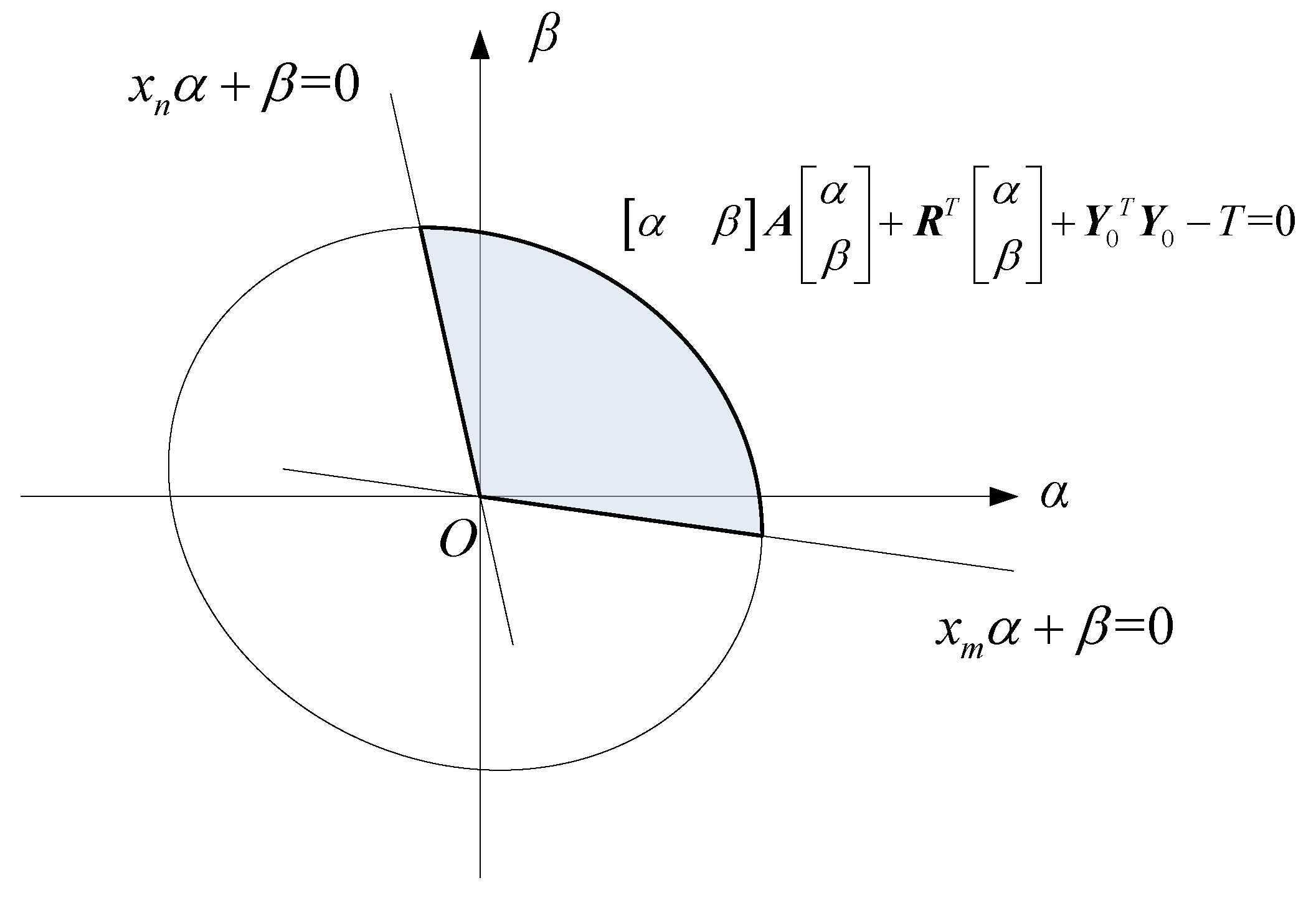
Since the determinant of A is greater than zero, the first condition of Equation (22) defines the inner region of an ellipse which is expressed as $\left[\begin{array}{cc}\alpha & \beta \end{array}\right]A\left[\begin{array}{c}\alpha \\ \beta \end{array}\right]+R^T\left[\begin{array}{c}\alpha \\ \beta \end{array}\right]+Y_0{}^T{Y}_0-T=0$. Assuming that x_m is maximum among X and x_n is minimum among X, the second condition is made up of the area enclosed by the upside of $x_m\alpha +\beta =0$ and $x_n\alpha +\beta =0$. The restricted condition enclosed area is shown in Figure 8.

Equation (22) can be simplified to

$$\begin{array}{ll}\min & S=\left[\begin{array}{cc}\alpha & \beta \end{array}\right]H\left[\begin{array}{c}\alpha \\ \beta \end{array}\right]+P^T\left[\begin{array}{c}\alpha \\ \beta \end{array}\right]+\Phi \\ S.T.& \\ & f(\alpha ,\beta )=\left[\begin{array}{cc}\alpha & \beta \end{array}\right]A\left[\begin{array}{c}\alpha \\ \beta \end{array}\right]+R^T\left[\begin{array}{c}\alpha \\ \beta \end{array}\right]+Y_0{}^T{Y}_0\le T\\ & g(\alpha ,\beta )=\left[\begin{array}{cc}-x_n& -1\\ -x_m& -1\end{array}\right]\left[\begin{array}{c}\alpha \\ \beta \end{array}\right]\le 0\end{array}.$$

(25)

The minimum value of S must be obtained on the boundary of the constraint conditions. At this time, we can use Rockafellar Multiplier optimization Equation (25). In order to use the Rockafellar Multiplier optimization function, we must find a feasible initial point in the feasible region. The method of selecting initial points is as follows. Firstly, we should find the center of the ellipse $x_0$.

$$\left[\begin{array}{c}{x}_0\\ 1\end{array}\right]=\eta {\left[\begin{array}{cc}A& R\\ R^T& Y_0{}^T{Y}_0-T\end{array}\right]}^{-1}\left[\begin{array}{c}0\\ 0\\ 1\end{array}\right],$$

(26)

${\left[\begin{array}{cc}{x}_0& 1\end{array}\right]}^T$ is the homogeneous coordinates of $x_0$, $\eta$ is the arbitrary constant. If $x_0={\left[\begin{array}{cc}u& v\end{array}\right]}^T$, intersection of $\beta =v$ and $x_m\alpha +\beta =0$, $x_n\alpha +\beta =0$ are respectively p1 and p2. The intersection in the feasible region is the initial value of the Rockafellar Multiplier optimization Equation (25).

Equation (25) of the Jacobian matrix and Hessian matrix respectively are

$${\nabla }_{\left[\begin{array}{cc}\alpha & \beta \end{array}\right]}S=2\left[\begin{array}{cc}\alpha & \beta \end{array}\right]H+P^T,$$

(27)

$${\nabla }_{\left[\begin{array}{cc}\alpha & \beta \end{array}\right]}{}^{2}S=2H,$$

(28)

$${\nabla }_{\left[\begin{array}{cc}\alpha & \beta \end{array}\right]}f(\alpha ,\beta )=2\left[\begin{array}{cc}\alpha & \beta \end{array}\right]A+R^T,$$

(29)

$${\nabla }_{\left[\begin{array}{cc}\alpha & \beta \end{array}\right]}{}^{2}f(\alpha ,\beta )=2A,$$

(30)

$${\nabla }_{\left[\begin{array}{cc}\alpha & \beta \end{array}\right]}g(\alpha ,\beta )=\left[\begin{array}{cc}-x_n& -1\\ -x_m& -1\end{array}\right],$$

(31)

$${\nabla }_{\left[\begin{array}{cc}\alpha & \beta \end{array}\right]}{}^{2}g(\alpha ,\beta )=\mathbf{0}.$$

(32)

Based on the initial value and Equations (28)–(32), the optimal solution of Equation (25) can be obtained by the Rockafellar Multiplier.

4. Experimental Analysis

In order to verify the robustness and effectiveness of the proposed algorithm, this paper conducted two groups of experiments. One group, through computer simulation of the noisy environment, compares the denoising results of different algorithms under the different noisy conditions by quantitative curves. The other group, using the physical image under different noisy environments, uses visual comparison to compare the denoising results of different algorithms.

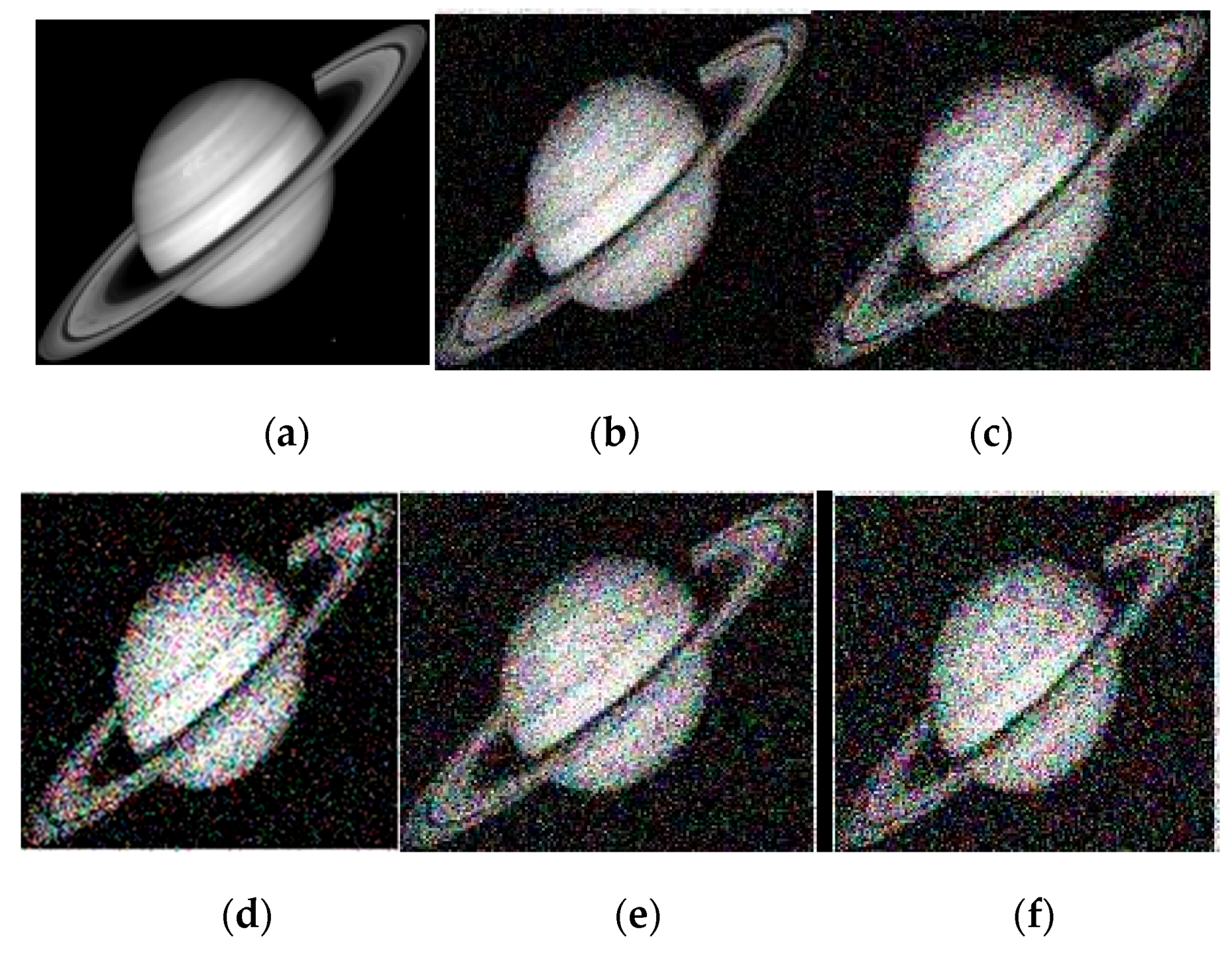
4.1. Computer Simulation Experiment

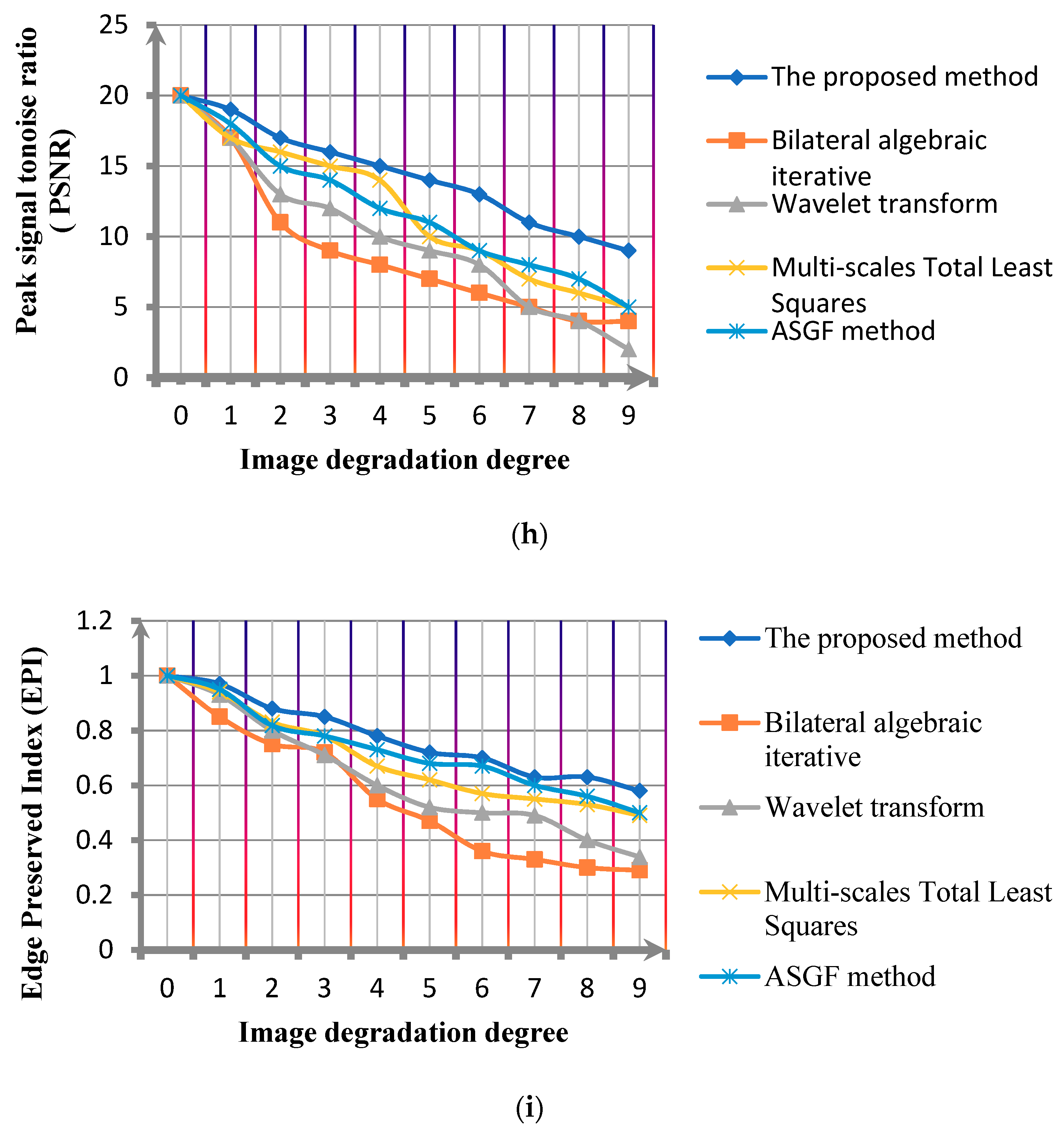
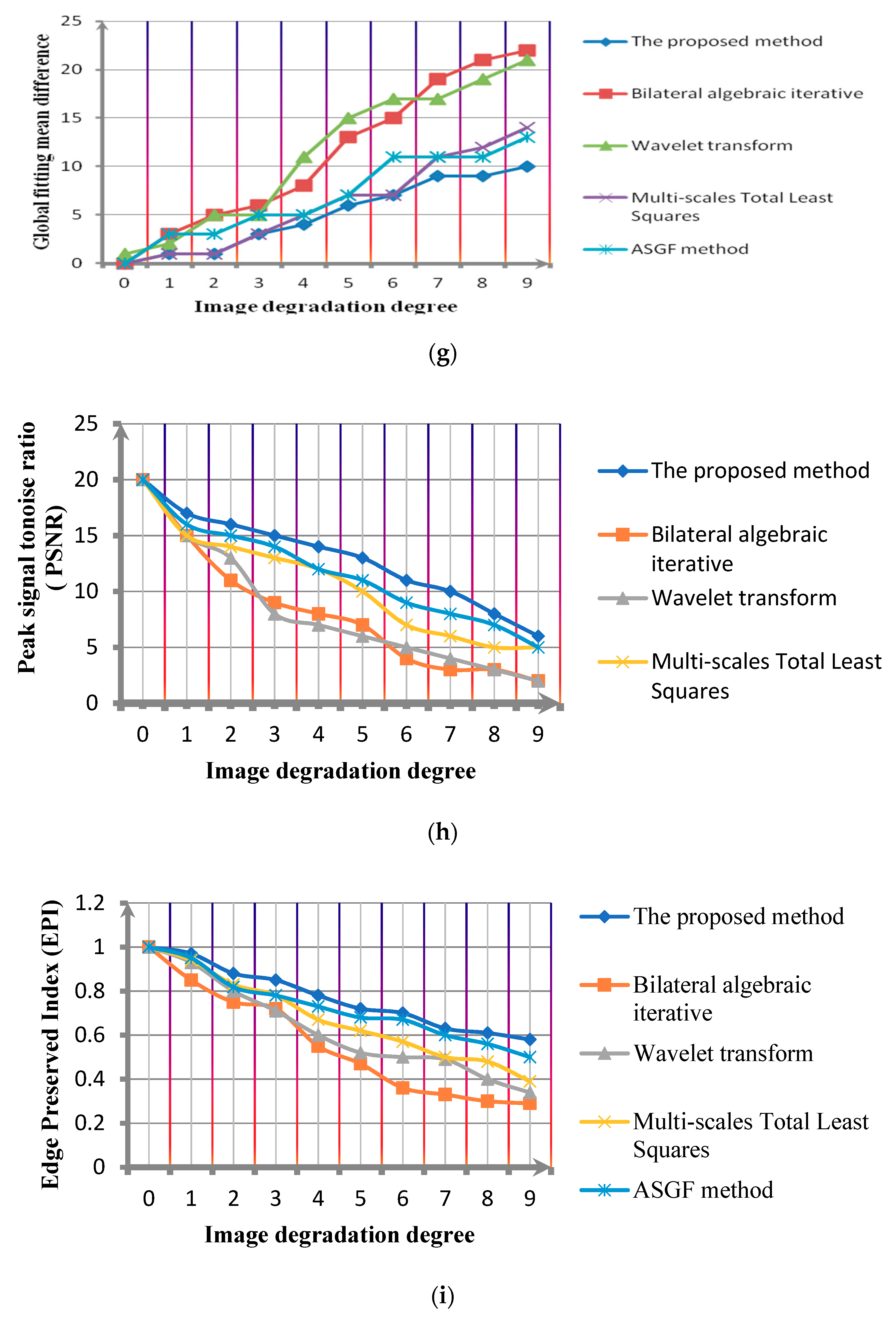
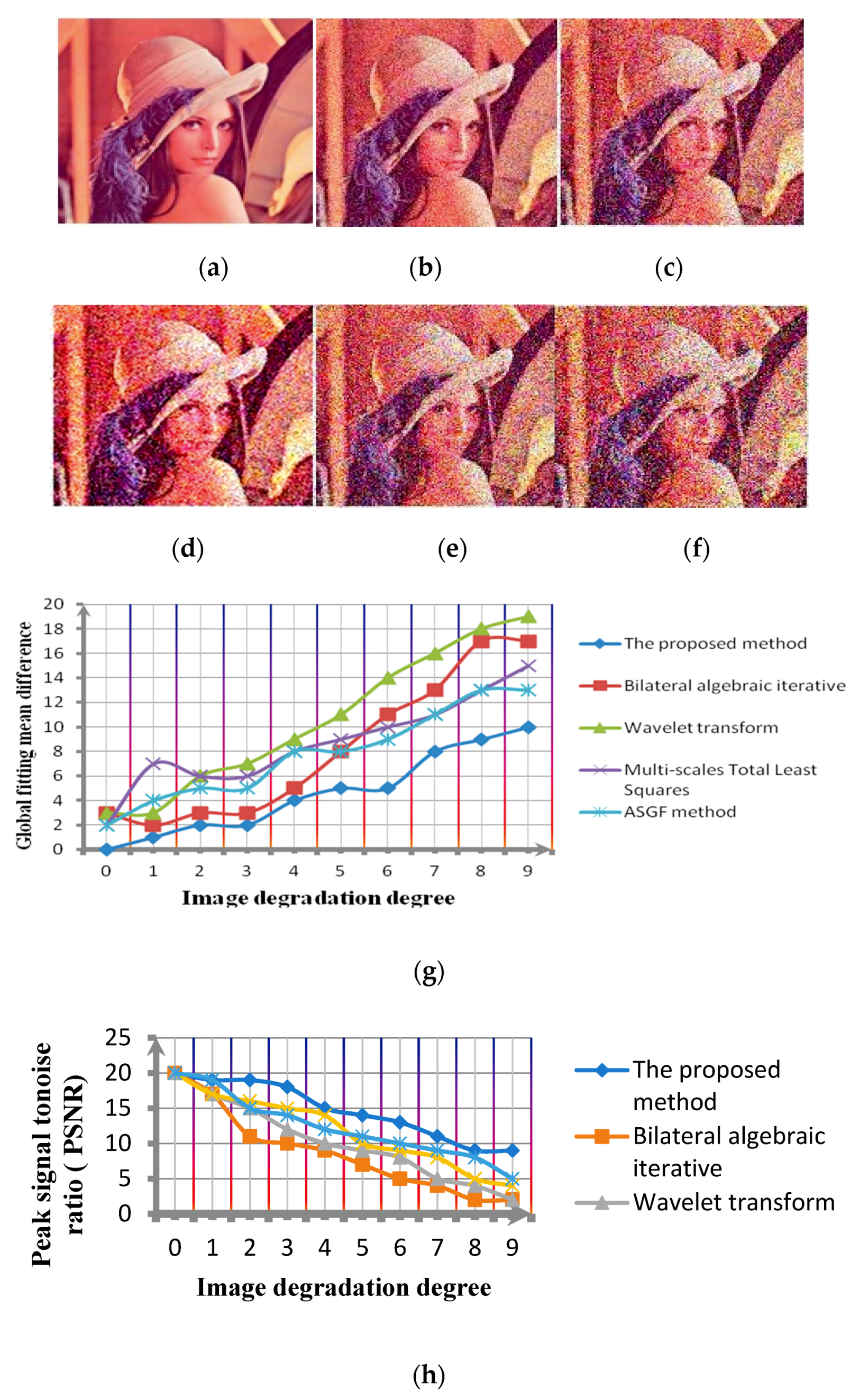
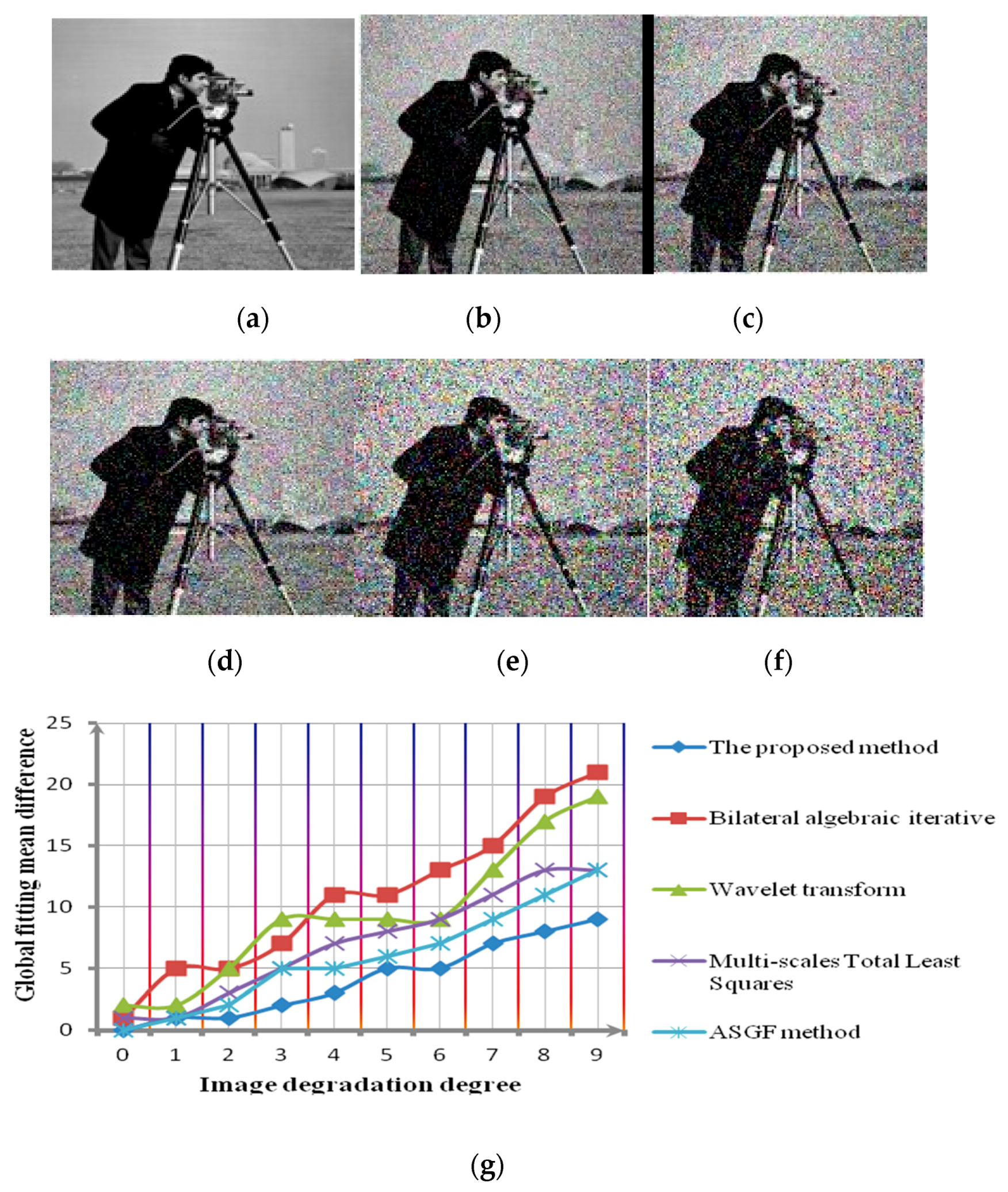
In this paper, in order to carry out the computer simulation experiment, we firstly reduce the quality of the known clear test image. Images with different SNR are divided into 10 groups. The 10 groups of test images were labeled as $\varsigma =0$, $\varsigma =1$, $\varsigma =2$, $\varsigma =3$, $\varsigma =4$, $\varsigma =5$, $\varsigma =6$, $\varsigma =7$, $\varsigma =8$, $\varsigma =9$. $\varsigma =0$ is the clear image and $\varsigma =9$ is the image with the lowest SNR. The denoising result is judged by the global fitting mean difference. This index is the average value of the pixel differences between the result and the original image.

Comparing the denoising experimental results with the Bilateral algebraic iterative method, wavelet transform, Multi-scales Total Least Squares [37], Adaptive sparse gradients field method (ASGF method) [38] and the proposed method, the results are shown in Figure 9, Figure 10 and Figure 11. In addition, in order to reflect the performance difference between the proposed algorithm and the other algorithms more intuitively. 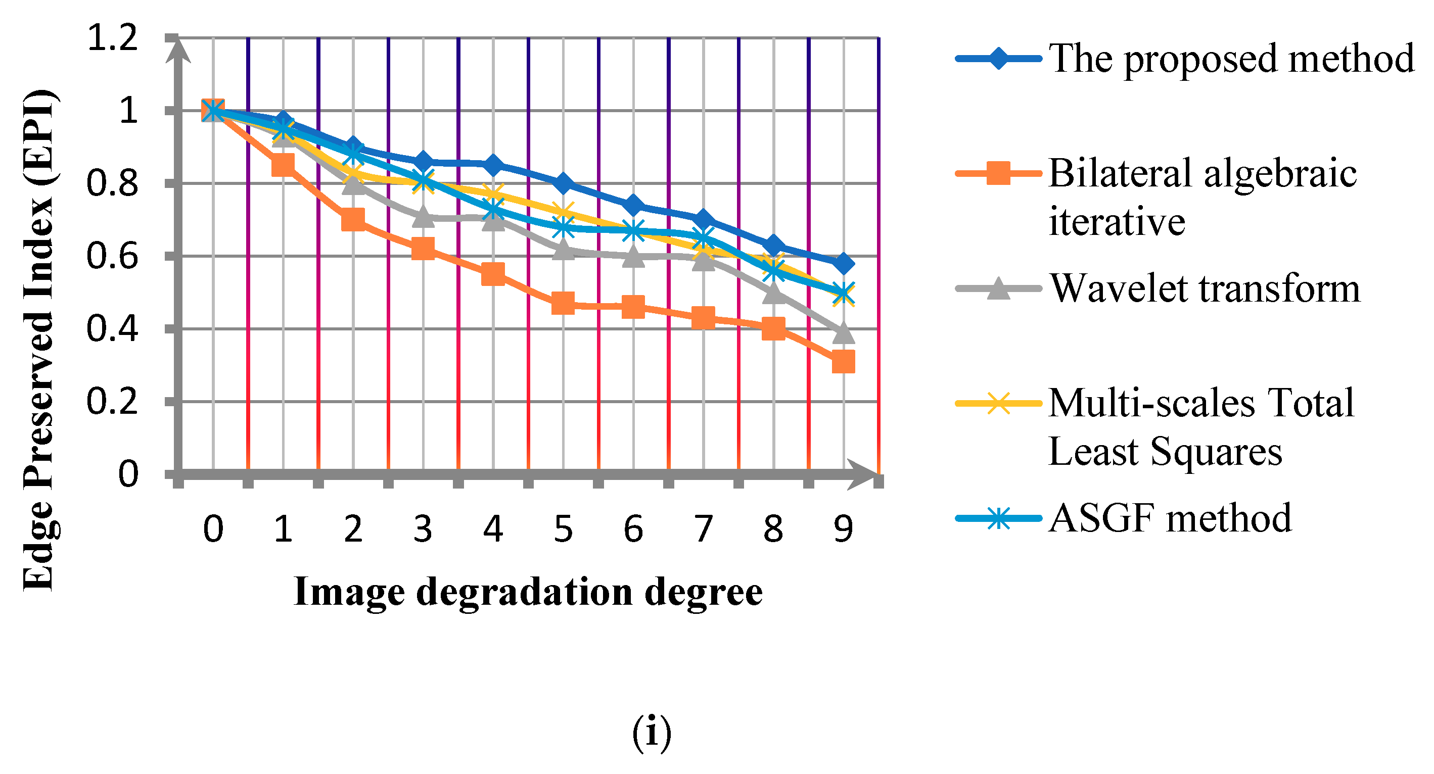Figure 9h,i, Figure 10h,i and Figure 11h,i show the comparison of the PSNR comparison and edge preserving index(EPI) of the algorithms under different noise standard deviations.

Over analysis can be obtained, comparing the Bilateral algebraic iterative method, Wavelet transform, Multi-scales Total Least Squares method and ASGF method. The global fitting mean difference of the proposed method is obviously minimal. That is to say, compared with other methods, the proposed method has a higher denoising robustness for images with different definitions. In addition, Figure 9h,i, Figure 10h,i and Figure 11h,i show that the proposed method has the advantage in improving the PSNR of the image and the image structure information preservation.

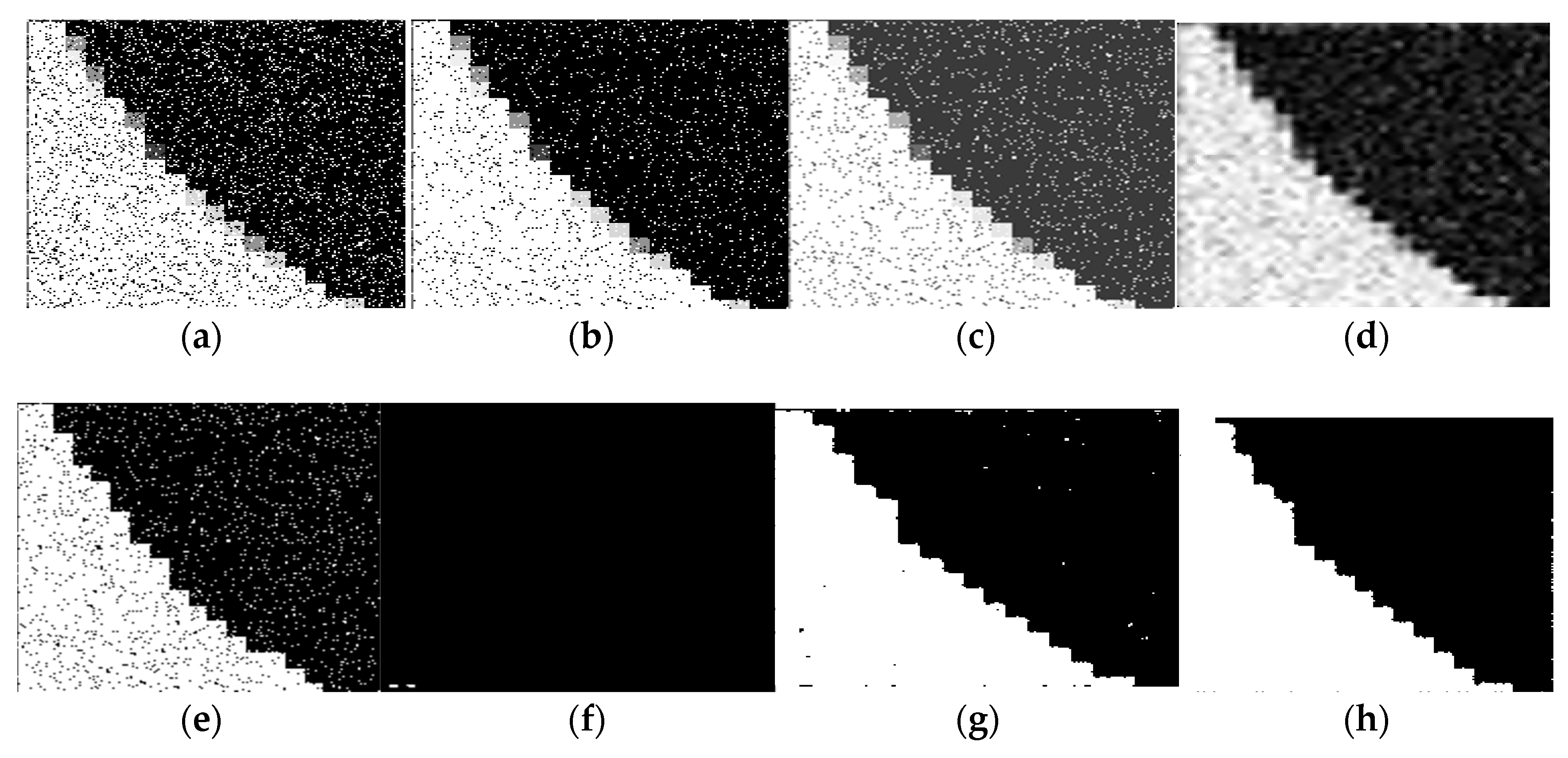
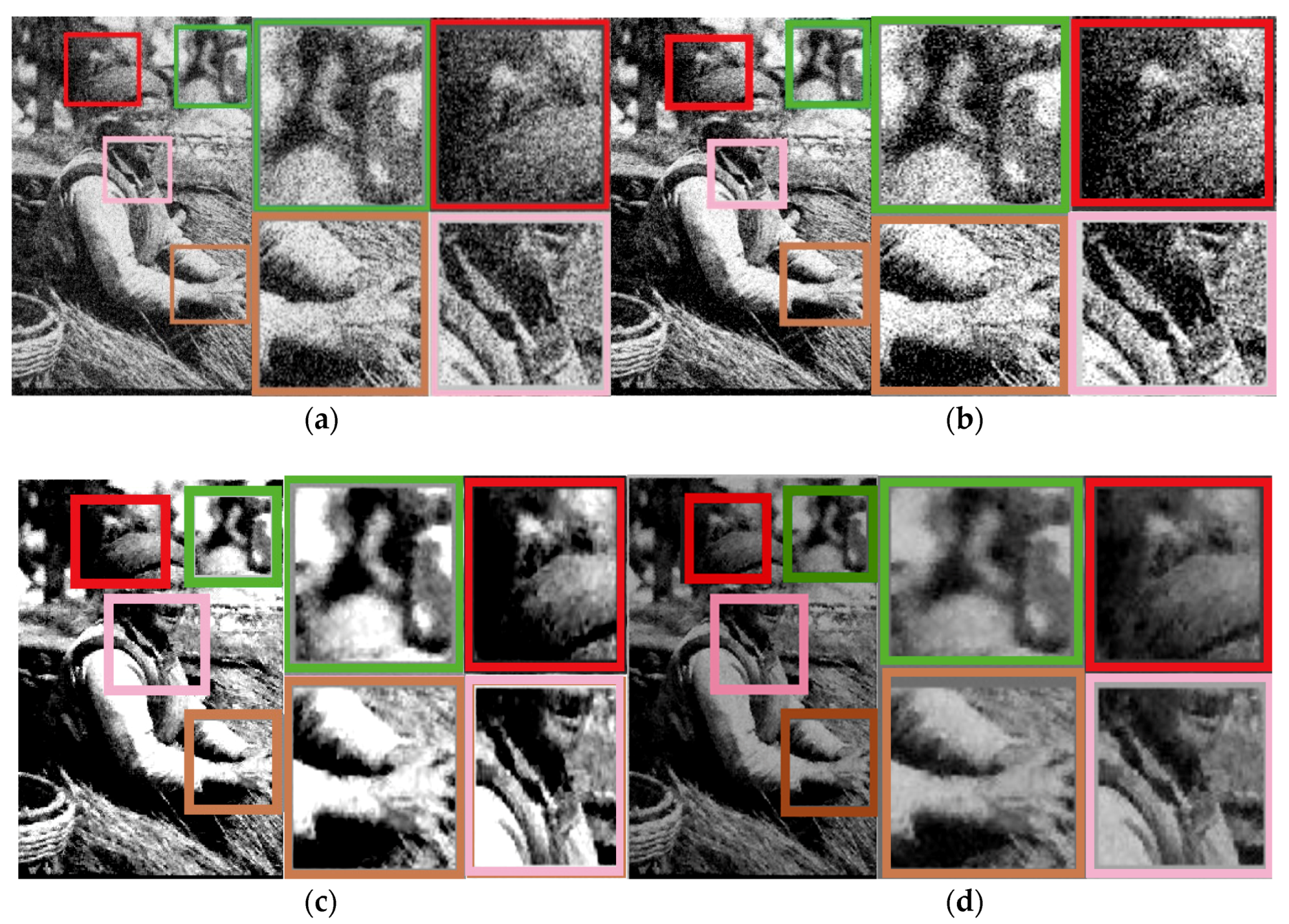
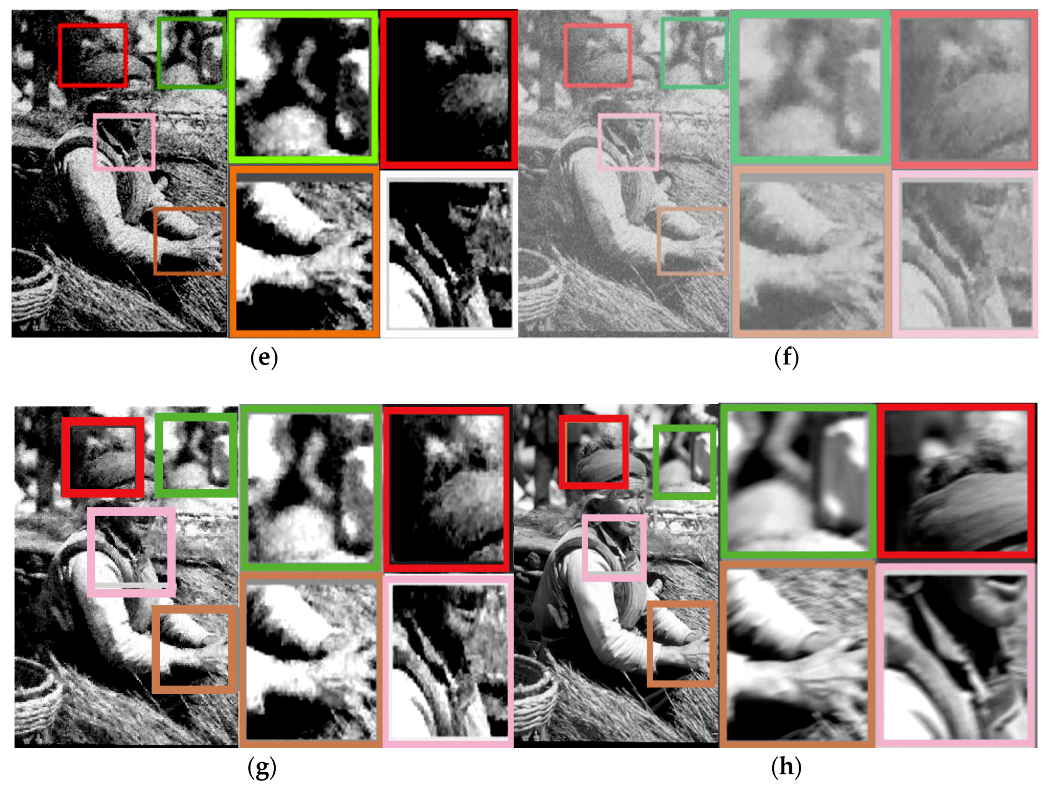
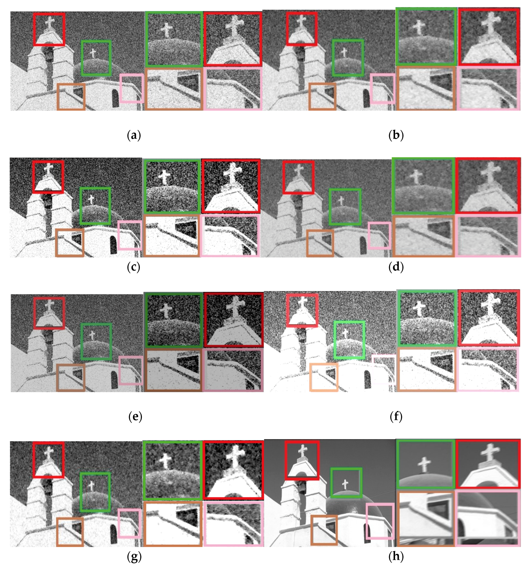
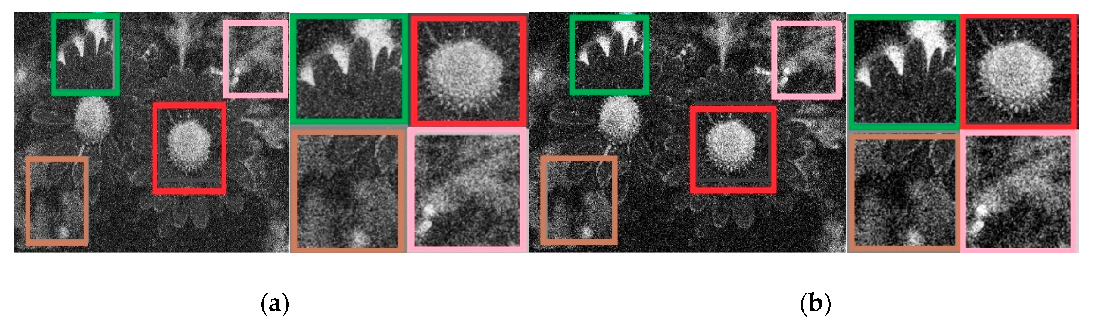
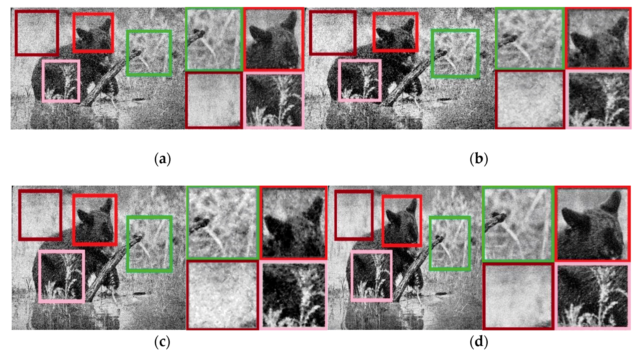
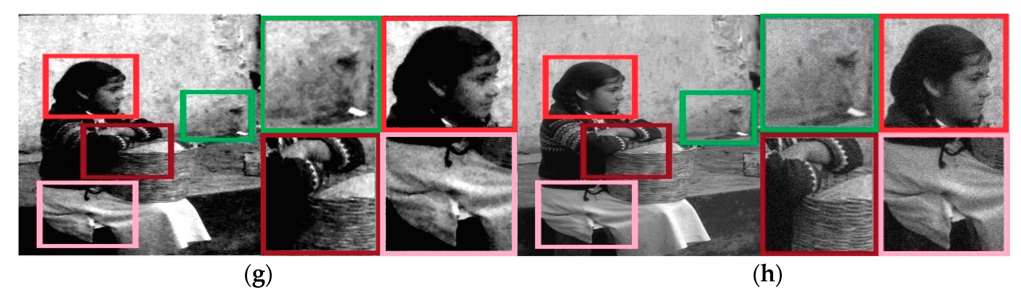
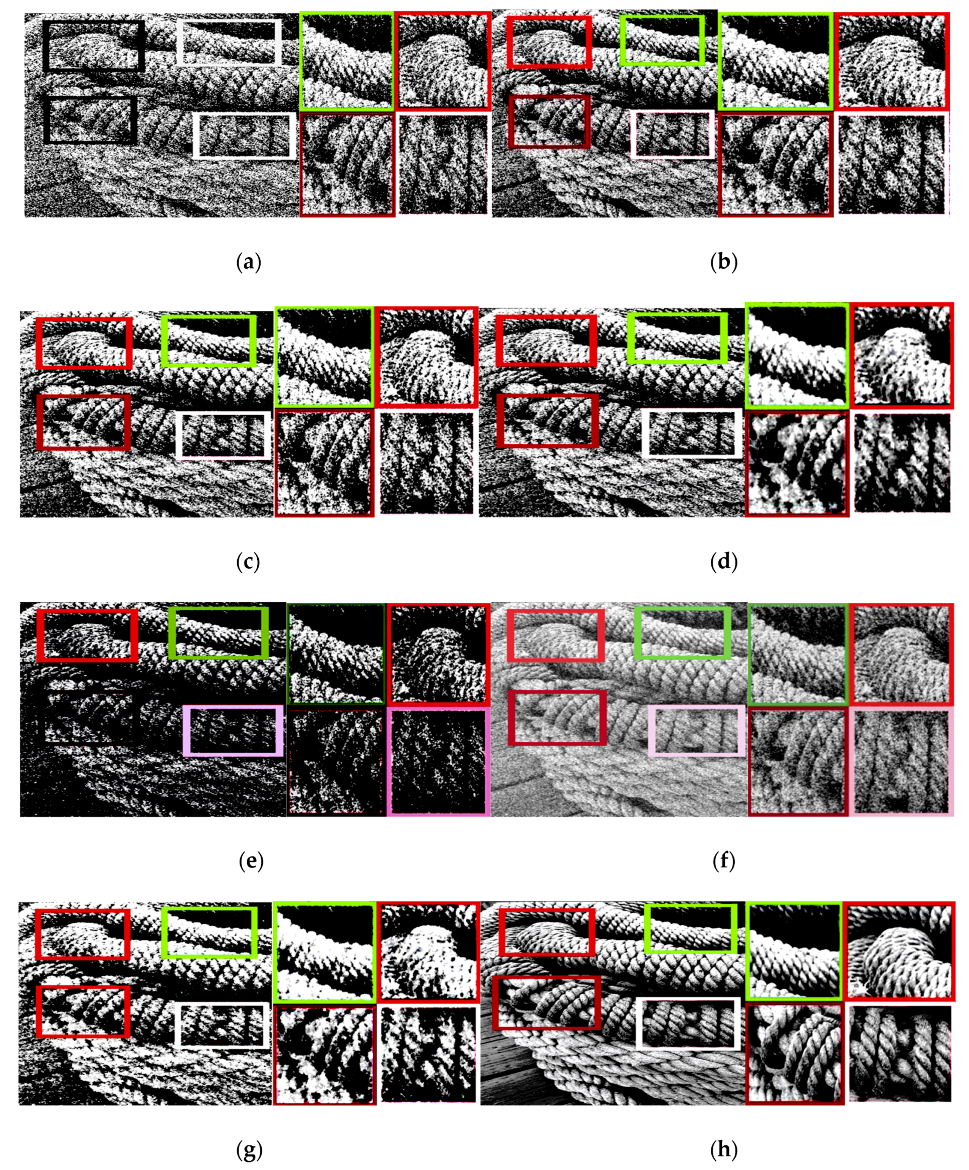
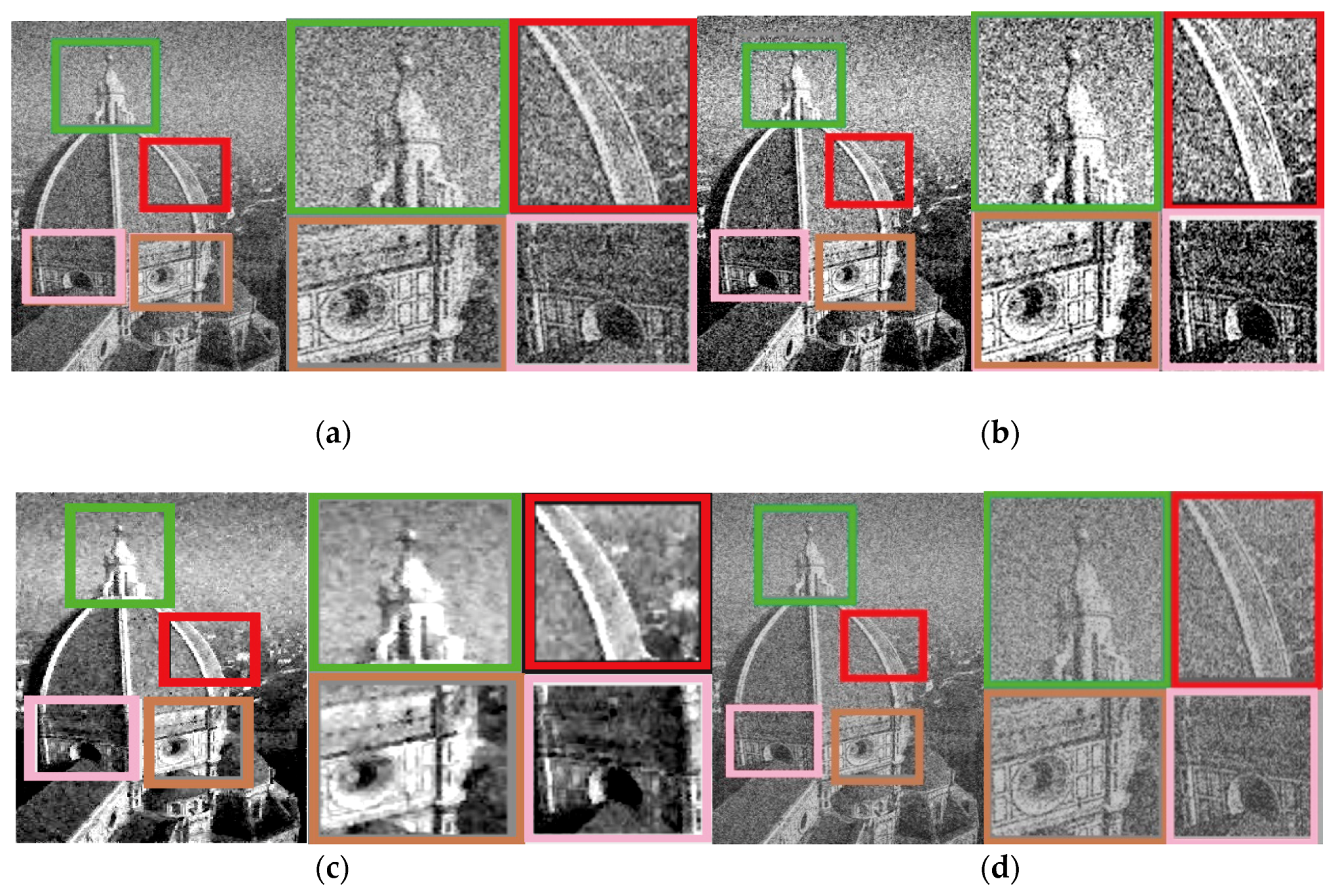
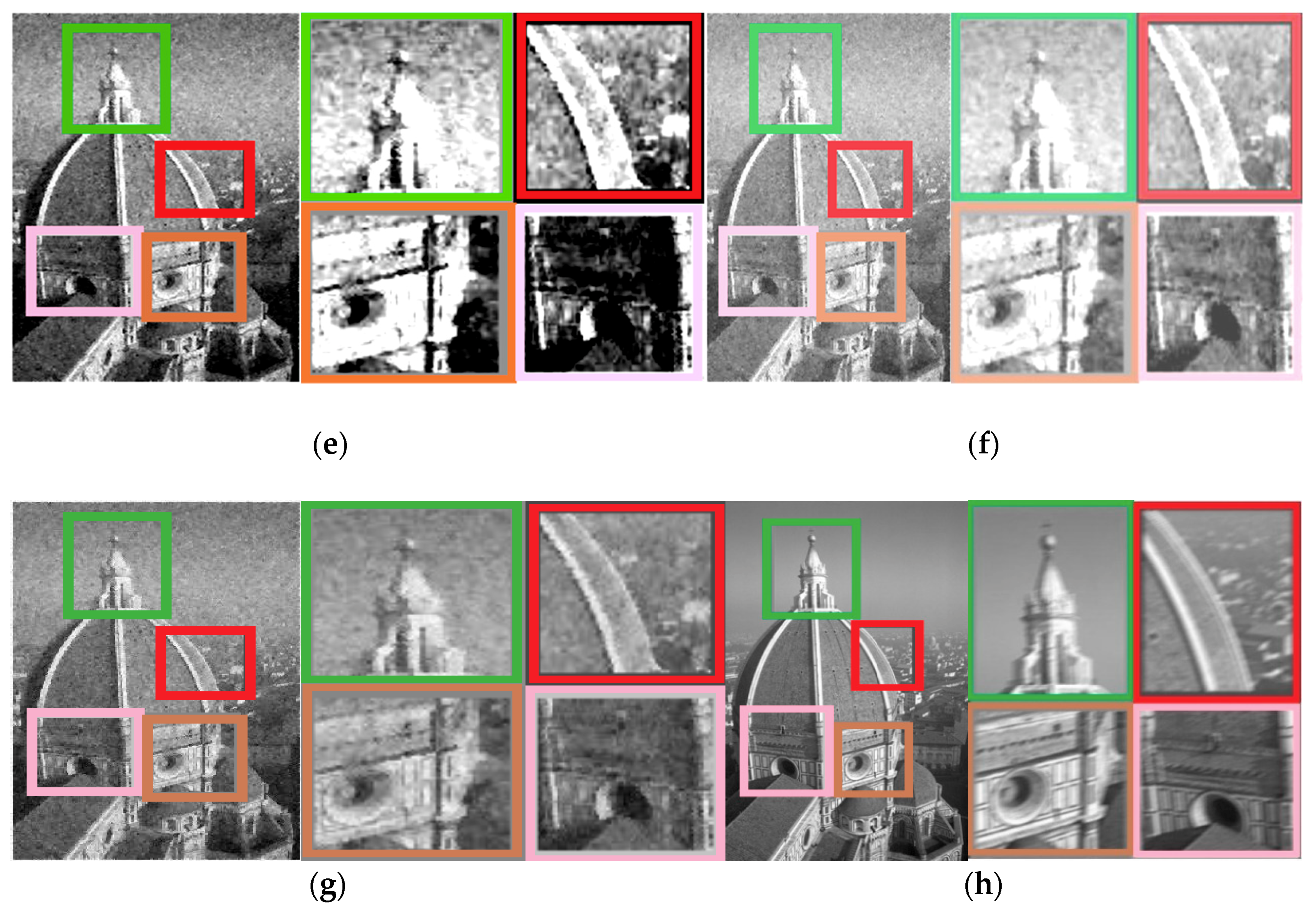
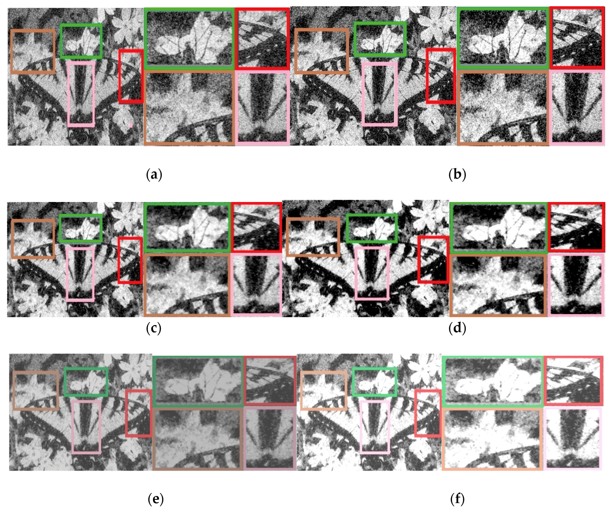
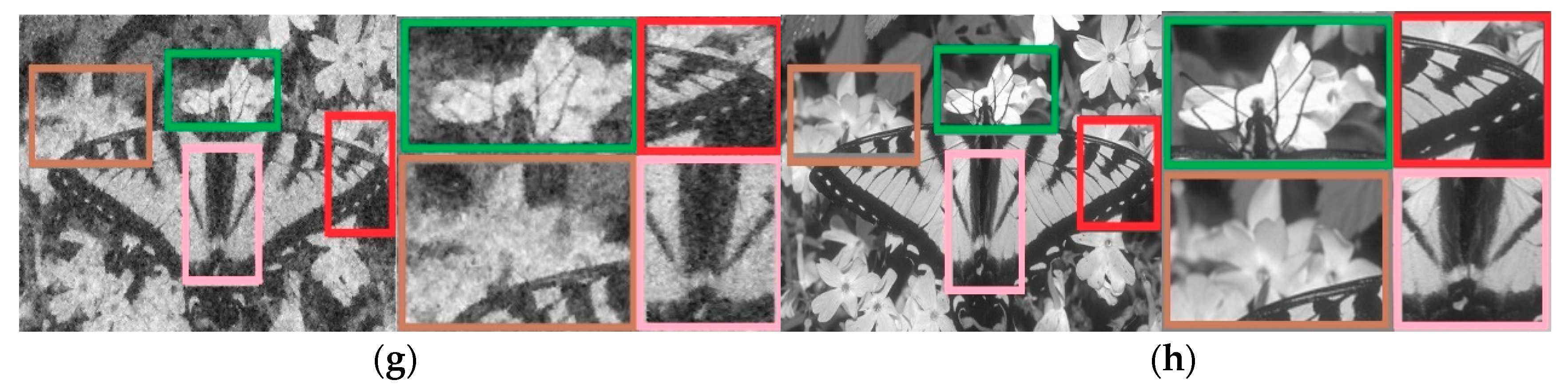
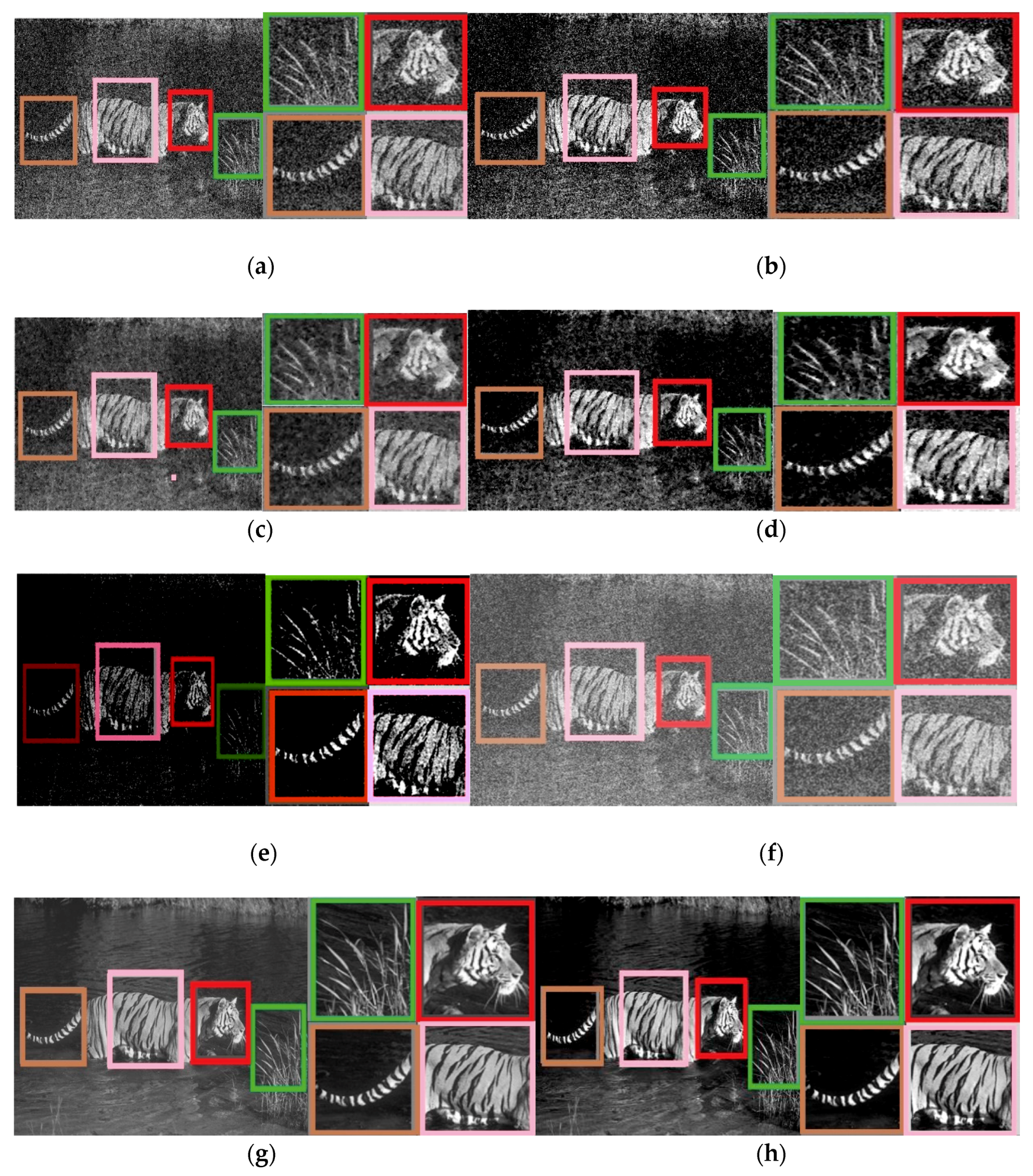
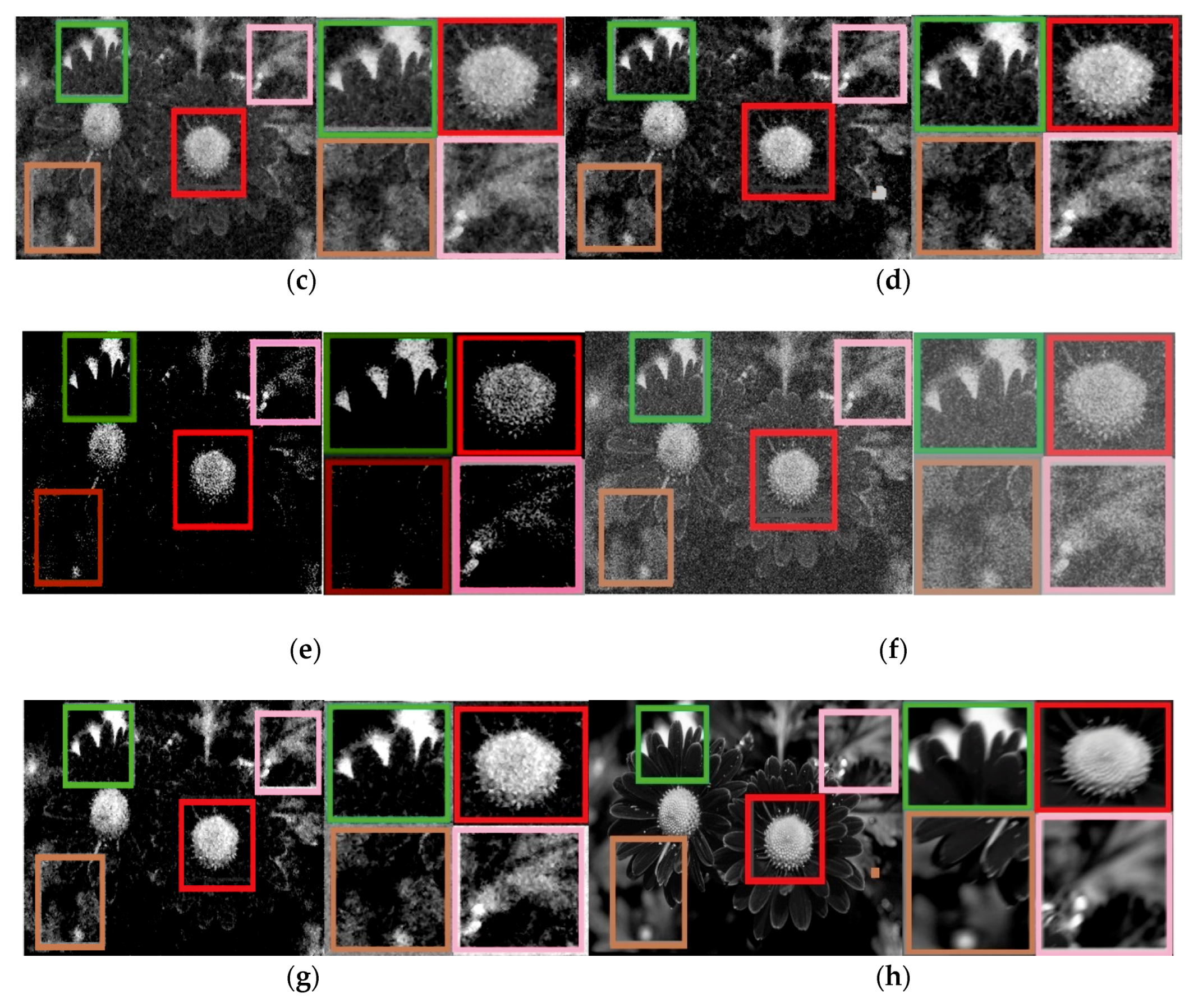
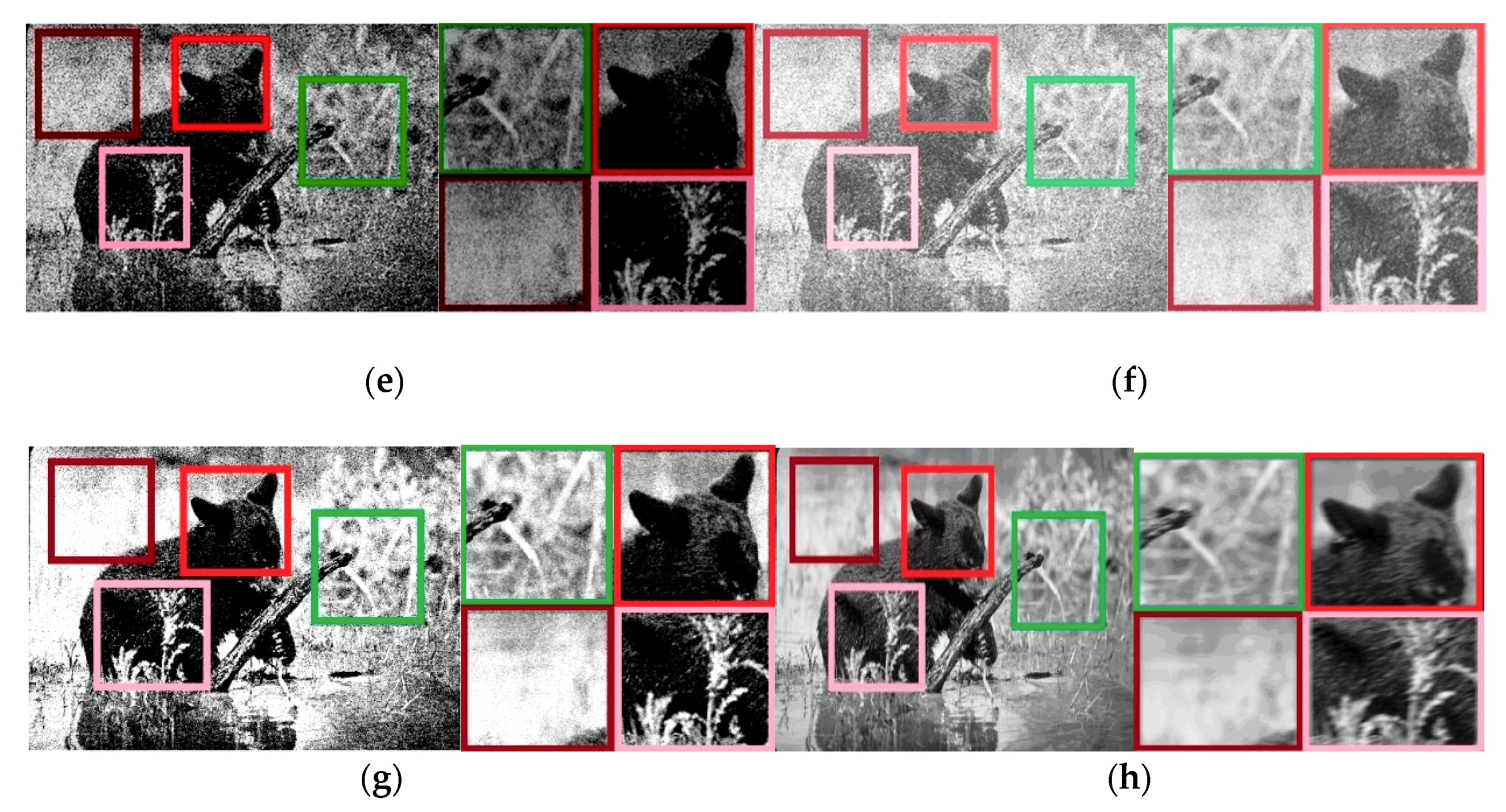
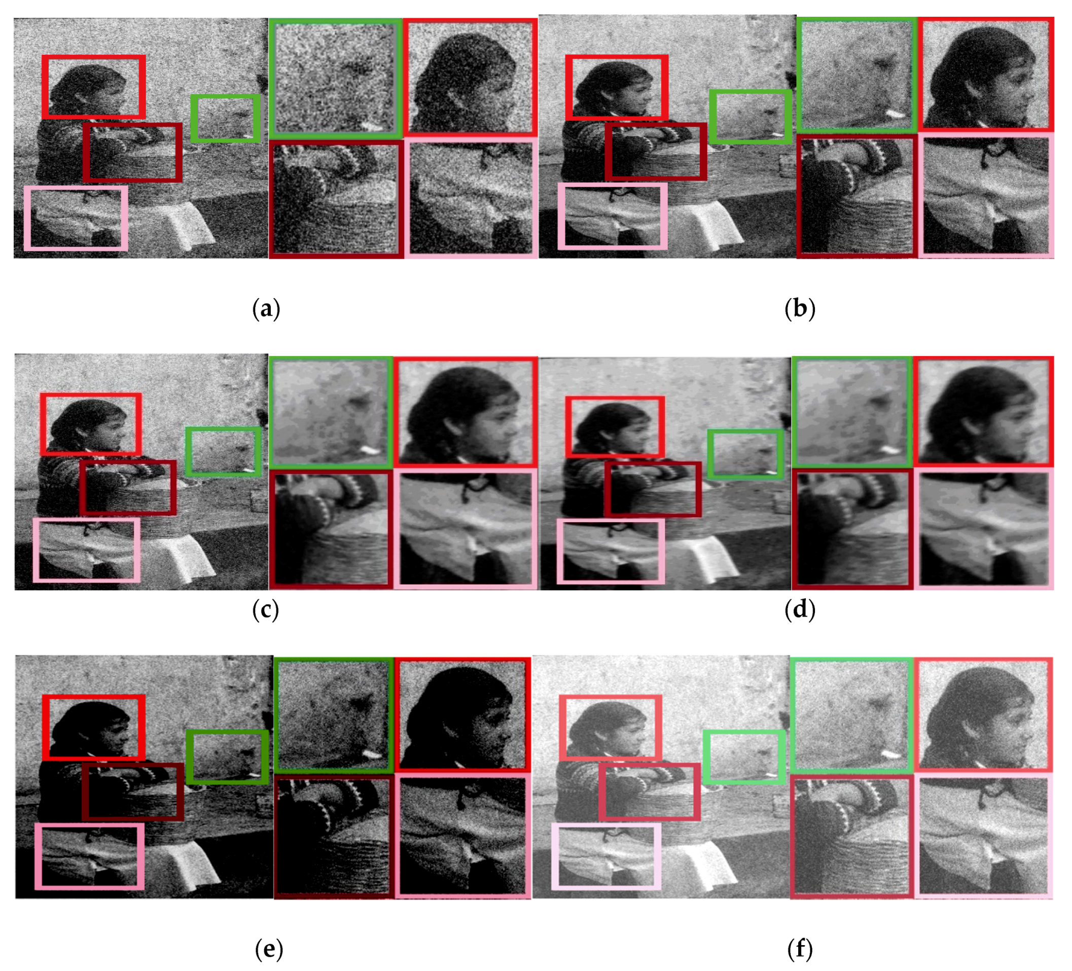
4.2. Physical Image Experiment

This paper uses 10 different types of images—A black and white edge map, a flower image, a straw rope image, two character images, two architectural images, and three animal images. Comparing the denoising experimental results with (b) Bilateral algebraic iterative method (BAI); (c) Wavelet transform (WT); (d) Multi-scales Total Least Squares (MTLS); (e) Adaptive sparse gradients field method (ASGF); (f) Region-aware image denoising algorithm (RAID); (g) Hilbert vibration decomposition (HVD) and (h) The proposed method. The results are shown in Figure 12, Figure 13, Figure 14, Figure 15, Figure 16, Figure 17, Figure 18, Figure 19, Figure 20 and Figure 21.

We can get the following conclusions by analyzing results. For the Bilateral iterative denoising algorithm, due to the uncertainty of the iterative initial value, the result is usually associated with the speckle noise belt in the denoising process. Then, in the process of iteration, there is no optimized reference data, which will lead to visual distortion. In addition, this classical method takes the pixel matrix of the entire image as an input. It usually disregards the geometric shapes of the target or interesting region. In this case, target edge information is fuzzy, which will be harmful to the following image analysis. The traditional wavelet denoising is used to put the noise into different scales under the multi resolution. If the threshold value is too high, it will cause serious loss of image detail. On the contrary, if the threshold value is too low, it will cause more noise not to be filtered. So it is the key to select the threshold when using wavelet denoising. In the case of serious noise pollution, threshold selection will be more difficult. The results of the wavelet denoising are not ideal.

Global least square method estimates the signal wavelet coefficients by total least square method and considers the correlation between different scale wavelet coefficients. It uses the optimizing wavelet threshold to reduce noise. Compared with classical methods, the denoising result of this method is obviously improved. However, it is difficult to determine the number of wavelet decomposition levels and it always need to be tuned artificially. Thus, both the scope of application and the definition of denoising are limited. Sparse gradients field denoising method provides an adaptive sparse gradients field (ASGF) model. This method solves the problem that the traditional gradient field is sensitive to noise. However, there are still problems that color fidelity is not enough for color image processing and the massive noise treatment effect is not ideal. For Region-aware image denoising algorithm (RAID), the effect depends mainly on exploring parameter preference; for random noisy images, the selection effect of this parameter is unstable, so the output of the result is unstable. Hilbert vibration decomposition (HVD) mainly depends on the convergence of different transform domains. When there is a pixel mutation in the image, the convergence will be unstable, and the denoising effect of the mutation region is not ideal.

In this paper, the proposed adaptive geometric non-means denoising method takes full account of geometric information. Besides, the method divides the center pixel and its neighborhood into continuous surface and section. Using nonlinear fitting theory, we can apply the method into any surfaces. The experimental results show that the proposed method has a wide range of application, high definition and high ability to restore the full information of the edge of the image.

Linear fuzzy index [39], definition [40] and standard deviation [41] are commonly used parameters for quantitative analysis of the image denoising effect. By calculating the size of the three parameters above, we quantitatively analyze the denoising performance of each algorithm. Make f (x, y) be the pixel value of each position in the image, the image size is M × N, then:

(1) linear fuzzy index measurement

$$\gamma (f_{En})=\frac{2}{mn}{\displaystyle \sum _{x=1}^m{\displaystyle \sum _{y=1}^n\min \{p_{xy},(1-p_{xy})\}}}.$$

(33)

where, $p_{xy}=\sin [\frac{\mathsf{\pi }}{2}\times (1-\frac{f(x,y)}{f_{\max }})]$ is the pixel for the image; f (x, y) is the gray value of the pixel p_xy; f_max is the maximum gray value of the image f.

Based on the linear fuzzy index measurement of spatial domain analysis, the denoising performance of different algorithms can be compared quantitatively. The smaller the value of $\gamma$, the better the denoising performance.

(2) Definition

$$Def=\frac{1}{MN}{\displaystyle \sum _{m=1}^{M-1}{\displaystyle \sum _{n=1}^{N-1}\sqrt{{[f(m+1,n)-f(m,n)]}^2+{[f(m,n+1)-f(m,n)]}^2}}}.$$

(34)

The contrast of the image and the contrast of the local details can be reflected by (34). The clearer the image, the greater the Def value is.

(3) Standard deviation

$${\sigma }_f={\{\frac{1}{MN}{{\displaystyle \sum _{x=1}^{M-1}{\displaystyle \sum _{y=1}^{N-1}[f(x,y)-\overline{f}]}}}^2\}}^{\frac{1}{2}}.$$

(35)

Among them, $\overline{f}$ represents the mean value of the gray level of the image. The larger the standard difference is, the more gray level distribution in the image will be. This indicates that the target image contains more details.

According to the above three functions, the quantitative analysis results for Figure 12 of the denoising effect of various algorithms are shown in

Table 1. The quantitative analysis results for Figure 12 of the denoising effect of various algorithms.

	Noisy Image	BAI	WT	MTLS	ASGF	RAID	HVD	The Proposed Method
$\gamma (f_{En})$	0.86	0.64	0.59	0.51	0.39	0.33	0.35	0.24
Def	6.33	7.98	6.89	9.11	9.98	9.19	10.09	11.21
${\sigma }_f$	62.78	71.57	73.4	81.05	89.30	88.86	79.25	95.76

.

It can be seen from Table 1, this paper presents an image performance index algorithm which was better than the other algorithms; this algorithm shows the best enhancement effect. For MSM algorithm, the definition of value is greater than the histogram equalization and partial differential equations, and the standard deviation of the values, indicating that the algorithm enhanced the edge contrast, but failed to highlight the details and enhance the texture. In the partial differential equations, there was a larger standard deviation of image clarity, but with the original approach, which shows that the algorithms can enhance the arts and details at the same time will damage the overall clarity and image edge contrast. In this paper, the edge enhancement and the detailed texture are both taken into account.

5. Conclusions

In this paper, we have discussed a new method to recover the image corrupted by random noise. In order to make a tradeoff between image denoising and detail maintenance, a novel non-local means approximation method is proposed to initially denoise the image by a weighted non-local approximation kernel function, and then with this initialization, the final restored image is determined by a novel nonlinear optimization under the constraint of intensity change. During the processing, each pixel’s value in the original image is replaced by the obtained optimal value so that the scene change does not influence the denoising results. Plenty of experiments manifest that the algorithm in this paper can effectively remove the noise, while maintaining as much image edge information as possible. In addition, because of strong adaptability, the proposed algorithm does not need manual modification for denoising parameters. The further effort will be focused on real-time performance, denoising efficiency and establishing a set of more complete criteria for image denoising evaluation.