Multiple-Image Encryption Algorithm Based on the 3D Permutation Model and Chaotic System

Abstract

Large numbers of images are produced in many fields every day. The content security of digital images becomes an important issue for scientists and engineers. Inspired by the magic cube game, a three-dimensional (3D) permutation model is established to permute images, which includes three permutation modes, i.e., internal-row mode, internal-column mode, and external mode. To protect the image content on the Internet, a novel multiple-image encryption symmetric algorithm (block cipher) with the 3D permutation model and the chaotic system is proposed. First, the chaotic sequences and chaotic images are generated by chaotic systems. Second, the sender permutes the plain images by the 3D permutation model. Lastly, the sender performs the exclusive OR operation on permuted images. The simulation and algorithm comparisons display that the proposed algorithm possesses desirable encryption images, high security, and efficiency.

1. Introduction

Massive electronic shooting devices can generate a huge mass of images in many fields every day, such as vehicular traffic, medical care, and commerce. According to a statistics report, millions of video monitors were installed for the Chinese sky net project. These electronic shooting devices can generate billions of traffic images every day. In the hospital, X-ray, CT, or MRI examinations for patients generate many medical images. The famous retail platform—Taobao website—possesses billions of commodity images. These massive images are always related to the business secrets and even national security. How to protect these images attracts the attention of many scientists and engineers.

To protect image security, the experts of multimedia security have presented a variety of image encryption algorithms. Wang et al. proposed an image encryption algorithm with mixed hash functions [1]. Chai et al. presented an image encryption algorithm using a chaotic system and compressive sensing [2]. Wu et al. presented a color image DNA encryption with an NCA map-based CML [3]. Gan et al. proposed an image encryption algorithm using S-boxes and a chaotic system [4]. Ahmad et al. presented an image encryption algorithm using SHA-512 and hyper-chaos [5]. Bashir et al. presented an image encryption algorithm with Lv’s hyper-chaotic system [6]. Hua et al. presented an image encryption algorithm with two-dimensional Logistic-Sine-coupling map (2D-LSCM) [7]. Wu et al. presented an image encryption algorithm with two-dimensional Henon-Sine map (2D-HSM) [8]. Nevertheless, these algorithms are single-image encryption algorithms, which cannot make full use of the features of massive images.

The experts of multimedia security have paid more attention to the multiple-image encryption (MIE) technology in recent years. To protect the optical images, they have designed some MIE algorithms. Liu et al. presented an MIE algorithm with an asymmetric cryptosystem [9]. Di et al. proposed an MIE algorithm by the phase retrieval [10]. Xiong et al. presented an MIE algorithm in the Fourier domain [11]. Zhang et al. presented an MIE algorithm with compressive sensing [12]. Li et al. designed an MIE algorithm with the lifting wavelet transform [13]. Deng et al. presented an MIE algorithm with the Fourier transform [14]. Yuan et al. proposed an MIE algorithm with a single-pixel detector [15]. However, these MIE algorithms are designed with the features of optical images, which are not suitable for encrypting the digital images. Therefore, they have also presented some MIE algorithms to protect digital images. Li et al. proposed an MIE algorithm in the wavelet transform domain [16]. However, the decryption image is lossy and only contains the low-frequency coefficients of the plain images. Zhang et al. proposed two MIE algorithms by scrambling mixed image elements [17,18]. These algorithms are very efficient, but they stimulate the block effect especially for the large size of the image blocks. Meanwhile, Zhang et al. proposed an MIE algorithm with DNA encoding [19]. This algorithm is secure, but it is a little complex for the DNA encoding and decoding operations. Suri et al. presented an MIE algorithm with Cramer’s rule [20]. Das et al. presented an MIE algorithm with genetic operators [21]. However, these two algorithms can only encrypt two plain images at once.

To simultaneously protect multiple images, this paper establishes a three-dimensional (3D) permutation model and then designs a novel MIE algorithm with the 3D permutation model. Simulation results display the superiority of the proposed algorithm.

The main contributions of this manuscript include the following. (1) Inspired by the magic cube game, we establish a 3D permutation model, which includes three permutation modes, i.e., internal-row mode, internal-column mode, and external mode. (2) We propose an MIE algorithm based on the 3D permutation model and chaotic system. (3) We compare the proposed algorithm with eight similar algorithms, i.e., Hua’s Algorithm, Wu’s Algorithm, Li’s algorithm, Zhang’s Algorithms 1, 2, and 3, Suri’s algorithm, and Das’s Algorithm. (4) Simulation results and algorithm analyses show the superiority of the proposed algorithm in terms of the security and efficiency.

The paper is organized as: Section 2 establishes a 3D permutation model and introduces the chaotic systems. Section 3 proposes a novel MIE algorithm. Section 4 describes eight existing algorithms. Section 5 is the experiment. The performance of the proposed algorithm are discussed in Section 6. Section 7 concludes the whole paper.

2. Theoretical Principle

2.1. 3D Permutation Model

Rubik’s cube is a famous 3D intelligence game, which was invented by a Hungarian professor named Rubik in 1974 [22]. It is also called the magic cube. Figure 1a–c show the magic cubes with three, four, and five orders, respectively. For the three-order magic cube, the blocks can be rotated in three different directions, as shown in Figure 2, and the number of its variation cases is 43,252,003, 274,489,856,000 in total. With the increase of the order, the difficult degree increases exponentially. Therefore, it is very difficult to successfully combine a magic cube for a layman.

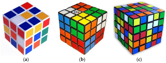
Figure 1. Magic cubes: (a) Three orders. (b) Four orders. (c) Five orders.

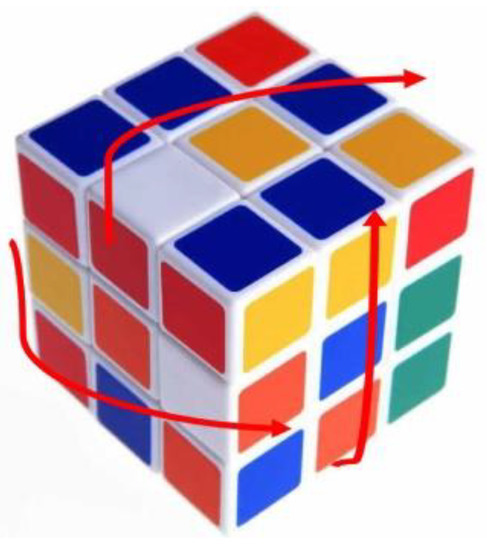
Figure 2. Magic cube rotation.

The image permutation and diffusion are two main means for the image encryption technology. The operation of image permutation only changes pixel positions. Conversely, the operation of image diffusion only changes pixel values. Inspired by the magic cube, we built a 3D permutation model for image encryption. For $k$ plain images with the same size $m\times n$, we can combine them into an image cube with the size $m\times n\times k$, which is shown in Figure 3. The pixel in the image cube is the counterpart of the block in the magic cube. Similarly, three permutation modes are designed for image encryption, i.e., internal-row mode, internal-column mode, and external mode. The first two modes permute pixel positions in one plain image. The last mode permutes pixel positions among all the plain images. These modes are described in detail below.

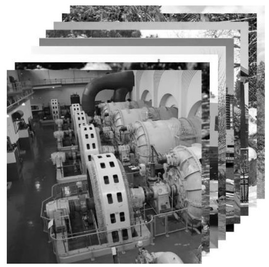
Figure 3. Image cube.

(1) Internal-row mode: for a plain image $I_{m\times n}^1$, its pixels are listed in $m$ rows. To permute its pixel positions, a random number $r_i\in \{1,2,\cdots ,n\}$, $i=1,2,\cdots ,m$ is chosen for every row. A random sequence ${\left\{r_i\right\}}_m$ can be generated by the chaotic system here. For the $i$th-row pixels, this mode performs the cyclic-shift operation with $r_i$ pixel positions to the right or left directions. If the sender performs the cyclic-shift operation to the right direction at the encryption stage, then the recipient should carry out the same operation to the left direction at the decryption stage. Otherwise, the recipient should carry out the same operation to the right direction at the decryption stage.

(2) Internal-column mode: for a plain image $I_{m\times n}^1$, its pixels are listed in $n$ columns. Regarding its permute pixel positions, a random number $r_i\in \{1,2,\cdots ,m\}$, $i=1,2,\cdots ,n$ is chosen for every column. A random sequence ${\left\{r_i\right\}}_n$ can be generated by the chaotic system here. For the $i$th-columns pixels, this mode performs the cyclic-shift operation with $r_i$ pixel positions to the up or down directions. If the sender performs the cyclic-shift operation to the up direction at the encryption stage, then the recipient should carry out the same operation to the down direction at the decryption stage. Otherwise, the recipient should carry out the same operation to the up direction at the decryption stage.

(3) External mode: the size of plain images $I^1,I^2,\cdots ,I^k$ are $m\times n$. To permute their pixel positions, a random number $r_{ij}\in \left\{1,2,\cdots ,k\right\}$ is chosen for the pixel $I_{ij}^1\in I^1$. A random matrix $R={\left\{r_{ij}\right\}}_{m\times n}$ can be obtained by the chaotic system in this case. For the pixel $I_{ij}^1$, this mode performs the cyclic-shift operation with $r_{ij}$ pixel positions to the front or back directions. If the sender performs the cyclic-shift operation to the front direction at the encryption stage, then the recipient should carry out the same operation to the back direction at the decryption stage. Otherwise, the recipient should carry out the same operation to the front direction at the decryption stage.

2.2. Chaotic Systems

The two-dimensional (2D) Logistic map and the Piece-Wise Linear Chaotic Map (PWLCM) are two commonly used chaotic systems. They can generate chaotic sequences to encrypt images. In this paper, two chaotic sequences generated by two PWLCM systems are used to permute pixel positions with the internal-row and internal-column modes, respectively. At the same time, the 2D Logistic map can generate two chaotic sequences. One is used to permute pixel positions with the external mode. The other is used to diffuse the pixel values.

(1) The 2D Logistic map is defined by Equation (1) below [23].

$$\{\begin{array}{l}{x}_{n+1}=r_1{x}_n\left(1-x_n\right)+s_1{y}_n^2\\ y_{n+1}=r_2{y}_n\left(1-y_n\right)+s_2\left(x_n^2+x_n{y}_n\right)\end{array},$$

(1)

where $r_1$, $r_2$, $s_1$, and $s_2$ are parameters to control the chaotic behavior. When $2.75<r_1\le 3.4$, $2.75<r_2\le 3.45$, $0.15<s_1\le 0.21$, and $0.13<s_2\le 0.15$, Equation (1) can generate two chaotic sequences. Its initial values $x_0,y_0$ and $r_1,r_2,s_1,s_2$ are keys for the proposed algorithm.

(2) PWLCM is defined by Equation (2) below [24].

$$z_{i+1}=F_p(z_i)=\{\begin{array}{l}\begin{array}{cc}\frac{z_i}{p}& 0\le z_i<p\end{array}\\ \begin{array}{cc}\frac{z_i-p}{0.5-p}& p\le z_i<0.5\end{array}\\ \begin{array}{cc}{F}_p(1-z_i)& 0.5\le z_i<1\end{array}\end{array},$$

(2)

where $z_i\in [0,1)$ and $p\in (0,0.5)$. Its initial value $z_0$ and $p$ are keys for the proposed algorithm.

3. Proposed MIE Algorithm

3.1. Key Generation

Secure hash algorithm (SHA) is a type of hash functions. SHA is primarily designed for the integrity services [25]. SHA-256 is widely used and its output is a 256-bit hash value. The proposed algorithm uses SHA-256 to generate keys as follows. To further improve the efficiency, users can use other much faster hash functions (such as Message Digest Algorithm-5, MD5) to substitute for SHA-256.

The proposed algorithm uses SHA-256 to generate the 256-bit hash value $K$ of $k$ plain images.

$$K=k_1{k}_2\cdots k_i\cdots k_{32},$$

(3)

where $k_i$, $i=1,2,\cdots ,32$ are 8-bit blocks.

One 2D Logistic map and two PWLCM systems are used in the proposed algorithm. The initial values $x_0,y_0$ and control parameters $r_1,r_2,s_1,s_2$ of the 2D Logistic map are calculated by using the equations below.

$$x_0=\frac{k_1\oplus k_2\oplus k_3}{255},$$

(4)

$$y_0=\frac{k_4\oplus k_5\oplus k_6}{255},$$

(5)

$$r_1=2.75+\frac{k_7\oplus k_8\oplus k_9}{255}\times 0.65,$$

(6)

$$r_2=2.75+\frac{k_{10}\oplus k_{11}\oplus k_{12}}{255}\times 0.7,$$

(7)

$$s_1=0.15+\frac{k_{13}\oplus k_{14}\oplus k_{15}}{255}\times 0.06,$$

(8)

$$s_2=0.13+\frac{k_{16}\oplus k_{17}\oplus k_{18}}{255}\times 0.02,$$

(9)

where $\oplus$ denotes the exclusive OR (XOR) operation in the binary system. The initial values $z_0^1,z_0^2$ and control parameters $p^1,p^2$ of two PWLCM systems are calculated by using the formulas below.

$$z_0^1=\frac{k_{19}\oplus k_{20}\oplus k_{21}\oplus k_{22}}{255},$$

(10)

$$z_0^2=\frac{k_{23}\oplus k_{24}\oplus k_{25}\oplus k_{26}}{255},$$

(11)

$$p^1=\frac{k_{27}\oplus k_{28}\oplus k_{29}}{255}\times 0.5,$$

(12)

$$p^2=\frac{k_{30}\oplus k_{31}\oplus k_{32}}{255}\times 0.5.$$

(13)

3.2. Alice’s Encryption Process

Figure 4 is the encryption flowchart. First, $k$ plain images are scrambled with the 3D permutation model. Second, $k$ permuted images are diffused with the XOR operation. For an easy description, the sender and recipient are named as Alice and Bob, respectively. The encryption steps are described in detail as follows.

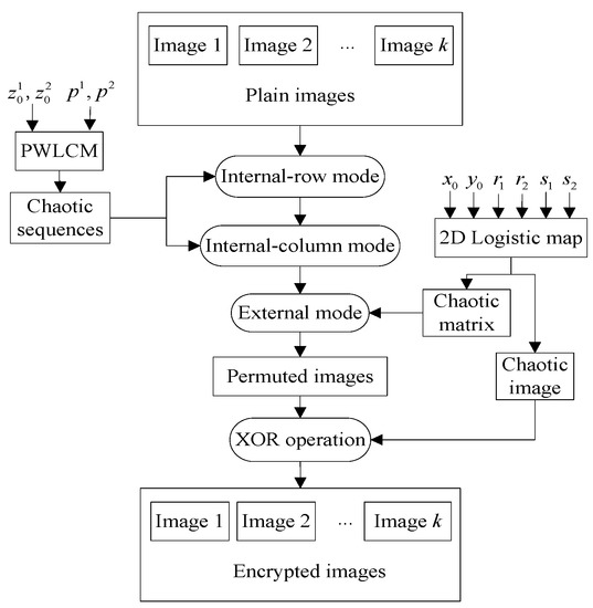
Figure 4. The encryption flowchart of the proposed algorithm.

Step 1: Generating the Key

$k$ plain images are $I^1,I^2,\cdots ,I^k$, whose sizes are $m\times n$. She computes the variables $x_0,y_0,r_1,r_2,s_1,s_2$ of the 2D Logistic map and the variables $z_0^1,z_0^2,p^1,p^2$ of two PWLCM systems with the method described in Section 3.1.

Step 2: Generating the Chaotic Sequence

The sender iterates PWLCM $m$ times with $z_0^1$ and $p^1$ and then obtains a chaotic sequence $Z^1={\left\{z_i^1\right\}}_m$. She computes

$$r_i^1=mod\left(floor\left(z_i^1\times {10}^{16}\right),m\right),$$

(14)

where $z_i^1\in Z^1$, $R^1={\left\{r_i^1\right\}}_m$, $floor(•)$ is the rounded-down function, and $\mathit{mod}(•)$ is the modulo operation. Similarly, she iterates PWLCM $n$ times with $z_0^2$ and $p^2$ and then obtains a chaotic sequence $Z^2={\left\{z_i^2\right\}}_n$. She computes

$$r_i^2=mod\left(floor\left(z_i^2\times {10}^{16}\right),n\right),$$

(15)

where $z_i^2\in Z^2$ and $R^2={\left\{r_i^2\right\}}_n$.

Step 3: Generating the Chaotic Image

Alice iterates the 2D Logistic map $m\times n$ times with $x_0,y_0,r_1,r_2,s_1,s_2$ and then obtains two chaotic sequences $X={\left\{x_i\right\}}_{mn}$ and $Y={\left\{y_i\right\}}_{mn}$. After that, she computes the following equations.

$$c_i^1=mod\left(floor\left(x_i\times {10}^{16}\right),k\right),$$

(16)

$$c_i^2=mod\left(floor\left(y_i\times {10}^{16}\right),256\right),$$

(17)

where $x_i\in X$ and $y_i\in Y$. Alice converts ${\left\{c_i^1\right\}}_{mn},{\left\{c_i^2\right\}}_{mn}$ into two $m\times n$ chaotic matrices $C^1,C^2$ respectively.

Step 4: Permutation with the Internal-Row Mode

Alice performs the permutation with the internal-row mode on the plain image $I^1$ with the chaotic sequence $R^1$. For the $i$th-row pixels, she performs the cyclic-shift operation with $r_i\in R^1$ pixel positions to the right direction. Similarly, she performs the permutation with the internal-row mode on $I^2,I^3,\cdots ,I^k$ with $R^1$. The permuted results are $I^{1\mathrm{r}},I^{2\mathrm{r}},\cdots ,I^{kr}$. In addition, Alice can enhance the algorithm security by a different chaotic sequence for a different plain image.

Step 5: Permutation with the Internal-Column Mode

Alice performs the permutation with the internal-column mode on $I^{1\mathrm{r}}$ with the chaotic sequence $R^2$. For the $i$th-column pixels, she performs the cyclic-shift operation with $r_i\in R^2$ pixel positions to the up direction. Similarly, she performs the permutation with the internal-column mode on $I^{2\mathrm{r}},I^{3\mathrm{r}},\cdots ,I^{kr}$ with $R^2$. The permuted results are $I^{1\mathrm{c}},I^{2\mathrm{c}},\cdots ,I^{kc}$. In addition, Alice can enhance the algorithm security by a different chaotic sequence for different $I^{1\mathrm{r}},I^{2\mathrm{r}},\cdots ,I^{kr}$.

Step 6: Permutation with the External Mode

Alice performs the permutation with the external mode on $I^{1\mathrm{c}},I^{2\mathrm{c}},\cdots ,I^{kc}$ with the chaotic matrix $C^1$. For the pixel $I_{ij}^{1c}\in I^{1\mathrm{c}}$, she performs the cyclic-shift operation with $c_{ij}\in C^1$ pixel positions to the front direction among $I^{1\mathrm{c}},I^{2\mathrm{c}},\cdots ,I^{kc}$. The permuted images are $I^{1\mathrm{e}},I^{2\mathrm{e}},\cdots ,I^{ke}$.

Step 7: Image Diffusion

To diffuse the images, Alice performs the XOR operation between $I^{1\mathrm{e}},I^{2\mathrm{e}},\cdots ,I^{ke}$ and $C^2$,

$$J^i=I^{ie}\oplus C^2,i=1,2,\cdots ,k.$$

(18)

The diffused results $J^1,J^2,\cdots ,J^k$ are the final encryption images.

3.3. Bob’s Decryption Process

Figure 5 is the image decryption flowchart. First, Bob performs the XOR operation on $k$ encrypted images. Second, he performs the inverse process of the 3D permutation model to recover the pixel positions. After Bob receives the keys $x_0,y_0,r_1,r_2,s_1,s_2,z_0^1,z_0^2,p^1,p^2$, he can decrypt $J^1,J^2,\cdots ,J^k$ with the following steps.

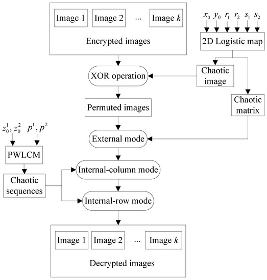
Figure 5. The decryption flowchart of the proposed algorithm.

Step 1: Generating the Chaotic Sequence

Bob iterates PWLCM $m$ times with $z_0^1$ and $p^1$ and then obtains a chaotic sequence $Z^1={\left\{z_i^1\right\}}_m$. $R^1={\left\{r_i^1\right\}}_m$ can be calculated with Equation (14). Similarly, he iterates PWLCM $n$ times with $z_0^2$ and $p^2$ and then obtains a chaotic sequence $Z^2={\left\{z_i^2\right\}}_n$. $R^2={\left\{r_i^2\right\}}_n$ that can be calculated with Equation (15).

Step 2: Generating the Chaotic Image

Bob iterates the 2D Logistic map $m\times n$ times with $x_0,y_0,r_1,r_2,s_1,s_2$ and then obtains two chaotic sequences $X={\left\{x_i\right\}}_{mn}$ and $Y={\left\{y_i\right\}}_{mn}$. According to the element positions and Equations (16) and (17), he can convert ${\left\{c_i^1\right\}}_{mn}$ into a chaotic matrix $C_{m\times n}^1$ and ${\left\{c_i^2\right\}}_{mn}$ into a chaotic image $C_{m\times n}^2$.

Step 3: Image Diffusion

Bob performs the XOR operation between $J^1,J^2,\cdots ,J^k$ and $C^2$,

$$I^{ie}=J^i\oplus C^2,i=1,2,\cdots ,k.$$

(19)

The diffused results $I^{1\mathrm{e}},I^{2\mathrm{e}},\cdots ,I^{ke}$ are the permuted images.

Step 4: Permutation with the External Mode

Bob performs the permutation with the external mode on $I^{1\mathrm{e}},I^{2\mathrm{e}},\cdots ,I^{ke}$ with the chaotic matrix $C^1$. For the pixel $I_{ij}^{1\mathrm{e}}\in I^{1\mathrm{e}}$, he performs the cyclic-shift operation with $c_{ij}\in C^1$ pixel positions to the back direction among $I^{1\mathrm{e}},I^{2\mathrm{e}},\cdots ,I^{ke}$. The permuted results are $I^{1\mathrm{c}},I^{2\mathrm{c}},\cdots ,I^{kc}$.

Step 5: Permutation with the Internal-Column Mode

Bob performs the permutation with the internal-column mode on $I^{1\mathrm{c}}$ and with the chaotic sequence $R^2$. For the $i$th-column pixels, he performs the cyclic-shift operation with $r_i\in R^2$ pixel positions to the down direction. Similarly, he performs the permutation with the internal-column mode on $I^{2\mathrm{c}},I^{3\mathrm{c}},\cdots ,I^{kc}$ with $R^2$. The permuted results are $I^{1\mathrm{r}},I^{2\mathrm{r}},\cdots ,I^{kr}$.

Step 6: Permutation with the Internal-Row Mode

Bob performs the permutation with the internal-row mode on the image $I^{1r}$ with the chaotic sequence $R^1$. For the $i$th-row pixels, he performs the cyclic-shift operation with $r_i\in R^1$ pixel positions to the left direction. Similarly, he performs the permutation with the internal-row mode on other images $I^{2\mathrm{r}},I^{3\mathrm{r}},\cdots ,I^{kr}$ with $R^1$. The permuted results are the decryption images $I^1,I^2,\cdots ,I^k$.

4. Existing Similar Algorithms

In the Introduction, References [1,2,3,4,5,6,7,8,9,10,11,12,13,14,15,16,17,18,19,20,21] are related to image encryption. However, the algorithms in References [1,2,3,4,5,6,7,8] are single-image encryption algorithms, which cannot encrypt multiple images at once. However, References [7,8] adopt the classical substitution-permutation network, which are similar to the proposed algorithm. Although the algorithms in References [9,10,11,12,13,14,15] are MIE algorithms, these MIE algorithms are designed with the features of optical images, which are not suitable for encrypting digital images. Therefore, this paper compares the proposed algorithm with the algorithms in References [7,8,16,17,18,19,20,21].

4.1. Hua’s Algorithm

Hua et al. proposed an image algorithm (short for Hua’s algorithm) [7]. The encryption steps are described as follows.

Step 1: Alice generates two chaotic matrices $S_{M\times N}$ and $R_{M\times N}$ with the 2D-LSCM.

Step 2: Alice simultaneously permutes the row and column positions of the plain image $P_{M\times N}$ in one operation and the permuted result is $T$.

Step 3: Alice diffuses $T$ by

$$C_i=\{\begin{array}{l}\begin{array}{cc}\left[T_1+T_G+T_{G-1}+floor(R_i\times 2^{32})\right]mod256& ifi=1\end{array}\\ \begin{array}{cc}\left[T_2+C_1+T_G+floor(R_i\times 2^{32})\right]mod256& ifi=2\end{array}\\ \begin{array}{cc}\left[T_1+C_{i-1}+C_{i-2}+floor(R_i\times 2^{32})\right]mod256& ifi\in [3,G]\end{array}\end{array},$$

(20)

where $C$ is the encrypted image, $G=N$ for the row diffusion, and $G=M$ for the column diffusion.

Step 4: Alice repeated Steps 2 and 3 with 4 rounds.

4.2. Wu’s Algorithm

Wu et al. proposed an image algorithm (short for Wu’s algorithm) [8]. The encryption steps are described below.

Step 1: the plain image is $P_{m\times n}$ and Alice computes $temp=\left({\displaystyle {\sum }_i{P}^i}\right)mod256$.

Step 2: Alice generates the chaotic sequences $x_1,y_1,x_2,y_2$ with the 2D-HSM and computes

$$R_x=round(x_1^i\times {10}^{10})mod8+1,$$

(21)

$$R_y=round(y_1^i\times {10}^{10})mod8+1,$$

(22)

$$R_z=round(x_2^i\times {10}^{10})mod8+1,$$

(23)

$$R=round(y_2^i\times {10}^{10})mod256,$$

(24)

where $round(•)$ is the function to obtain the nearest decimal or integer.

Step 3: Alice encodes $R,P$ with the rules $R_z,R_y$, respectively, and the encoded results are $DN{A}_R,DN{A}_P$.

Step 4: Alice computes

$$DN{A}_{P1}=DN{A}_P\otimes DN{A}_R,$$

(25)

where $\otimes$ denotes the DNA XOR operation.

Step 5: Alice decodes $DN{A}_{P1}$ with the rule $R_x$, and the encoded result is $New\_P$.

Step 6: Alice computes

$$D=New\_P\oplus temp,$$

(26)

where $D$ is the diffused result.

Step 7: Alice permutes $D$ with $x_1$ to get the encrypted image $C_{m\times n}$.

4.3. Li’s Algorithm

Li et al. proposed an MIE algorithm (short for Li’s algorithm) [16]. The encryption steps are described as follows.

Step 1: Alice performs the Discrete Wavelet Transform (DWT) for $k$ plain images and combines low-frequency coefficients into the reassembled image.

Step 2: Alice scrambles the reassembled image with the Arnold cat map to get the confused image.

Step 3: Alice segments the confused image into $k$ image blocks with an equal size.

Step 4: Alice scrambles, rotates, and diffuses these $k$ image blocks with the chaotic map.

Step 5: Alice reassembles the result of Step 4 into the encryption image.

4.4. Zhang’s Algorithm 1

Zhang et al. proposed an MIE algorithm (short for Zhang’s Algorithm 1) [17]. The encryption steps are described as follows.

Step 1: according to the given rule, Alice combines $k$ plain images into a big image. After that, she segments the big image into image blocks, i.e., pure image elements.

Step 2: Alice scrambles pure image elements with PWLCM to obtain the mixed image elements.

Step 3: Alice generates the big-scrambled image with the mixed image elements.

Step 4: Alice segments the big-scrambled image into $k$ encrypted images whose filenames are generated by PWLCM.

4.5. Zhang’s Algorithm 2

Zhang et al. proposed an MIE algorithm (short for Zhang’s Algorithm 2) [18]. The encryption steps are described below.

Step 1: Alice generates pure image elements.

Step 2: Alice scrambles pure image elements with PWLCM and then obtains the mixed image elements.

Step 3: Alice generates $k$ scrambled images with mixed image elements.

Step 4: to get the encryption images, Alice performs the XOR operation on $k$ scrambled images.

4.6. Zhang’s Algorithm 3

Zhang et al. proposed an MIE algorithm (short for Zhang’s Algorithm 3) [19]. The encryption steps are described below.

Step 1: according to the given rule, Alice encodes $k$ plain images with the DNA codes.

Step 2: Alice scrambles the DNA sequences of plain images with PWLCM.

Step 3: Alice segments the scrambled DNA sequence into $k$ parts and converts them into $k$ scrambled DNA matrices.

Step 4: Alice performs the DNA XOR operation between $k$ scrambled DNA matrices and the DNA matrix of the chaotic image generated by PWLCM and then obtains $k$ diffused DNA matrices.

Step 5: Alice decodes $k$ diffused DNA matrices to get the encryption images.

4.7. Suri’s Algorithm

Suri et al. proposed an MIE algorithm (short for Suri’s algorithm) [20]. The encryption steps are described as follows.

Step 1: Alice encrypts two plain images with two different methods. Image 1 is encrypted by AES and Image 2 is encrypted by a chaotic-based image encryption algorithm. Encrypted images 1 and 2 can be obtained.

In this paper, the size of two plain images is $m\times n$. For the chaotic-based image encryption algorithm, PWLCM is used to generate a chaotic sequence $X={\left\{x_i\right\}}_{m\times n}$. The integer chaotic sequence $Y={\left\{y_i\right\}}_{m\times n}$ can be calculated by $y_i=mod\left(floor\left(x_i\times {10}^{16}\right),256\right)$. Alice performs the XOR operation on Image 2 and $Y$. For the AES-based image encryption algorithm, Alice combines 16 pixel values to constitute the 128-bit data block and then uses AES-128 to encrypt the data block.

Step 2: inspired by the Cramer’s rule, Alice combines two encrypted images by using the formulas below.

$$I_1[i,j]=w_{11}\times I^{\prime }[i,j]+w_{12}\times I^{″}[i,j],$$

(27)

$$I_2[i,j]=w_{21}\times I^{\prime }[i,j]+w_{22}\times I^{″}[i,j],$$

(28)

where $w_{11},w_{12},w_{21},w_{22}$ are weights, $I^{\prime },I^{″}$ are the encrypted images in Step 1, and $I_1,I_2$ are the final encrypted images. In this paper, the weights are $w_{11}=0.63,w_{12}=0.37,w_{21}=0.32,w_{22}=0.68$.

4.8. Das’s Algorithm

Das et al. proposed an MIE algorithm (short for Das’s algorithm) [21]. The encryption steps are described as follows.

Step 1: the pixel values of two plain images $A={[a_{ij}]}_{m\times n}$ and $B={[b_{ij}]}_{m\times n}$ can be expressed with 8 bits in the binary form, i.e., $a_{ij}=a_{ij}^1{a}_{ij}^2\cdots a_{ij}^8$ and $b_{ij}=b_{ij}^1{b}_{ij}^2\cdots b_{ij}^8$;

Step 2: Alice performs the crossover operation (i.e., exchanging bits between the pixel values $a_{ij}$ and $b_{ij}$) and mutation operation (i.e., complementing bits for pixel values $a_{ij}$ and $b_{ij}$). The pixel values of diffused images $C1={[c{1}_{ij}]}_{m\times n}$ and $C2={[c{2}_{ij}]}_{m\times n}$ are $c{1}_{ij}=a_{ij}^1{a}_{ij}^2{a}_{ij}^r{b}_{ij}^{r+1}{b}_{ij}^{r+2}\cdots \sim b_{ij}^8$ and $c{2}_{ij}=b_{ij}^1{b}_{ij}^2{b}_{ij}^r{a}_{ij}^{r+1}{a}_{ij}^{r+2}\cdots \sim a_{ij}^8$ where $r\in \{1,2,\cdots ,8\}$ and $\sim$ denotes the complement operation. In this paper, $r$ is simulated with the element of the integer chaotic sequence $Y={\left\{y_i\right\}}_{m\times n}$ where $y_i=mod\left(floor\left(x_i\times {10}^{16}\right),8\right)+1$, $x_i\in X$ and $X$ is a chaotic sequence generated by PWLCM.

Step 3: Alice performs the XOR operation on the diffused images $C1$ and $C2$ pixel-by-pixel with a random set $E_k$ to get encrypted images. In this paper, $E_k$ is simulated by a chaotic image generated by PWLCM.

5. Experiments

The experimental purpose is to encrypt nine plain images with the same size $512\times 512$, as shown in Figure 6a–i, respectively. We developed the proposed algorithm, Hua’s algorithm, Wu’s algorithm, Li’s algorithm, Zhang’s Algorithms 1–3, Suri’s algorithm, and Das’s algorithm with Matlab R2016a.

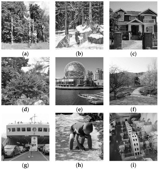
Figure 6. Plain images: (a) Tree. (b) Tiger. (c) House. (d) Flower. (e) Building. (f) Road. (g) Ship. (h) Boy. (i) Machine.

For the proposed algorithm, the big image is in Figure 7. Figure 6a–i constitute the first-row, second-row, and third-row image blocks of the big image, respectively. Therefore, the size of the big image is $1536\times 1536$. $K$ = 0x 36fad8690b3812a24c2fa1e50a9d727c74a1e a2a48bca87f7fa20f543a8b8fc5. With Equations (3)–(13), the variable values are $x_0$ = 0.07843137254902, $y_0$ = 0.352941176470588, $r_1$ = 3.392352941176471, $r_2$ = 3.043725490196079, $s_1$ = 0.203882352941176, $s_2$ = 0.143254901960784, $z_0^1$ = 0.203921568627451, $z_0^2$ = 0.039215686274510, $p^1$ = 0.190196078431373, and $p^2$ = 0.378431372549020.

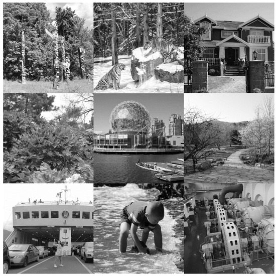
Figure 7. Big image.

For the proposed algorithm, the encryption images are shown in Figure 8a–i. The recipient can decrypt them with the decryption keys. The decrypted images are lossless, which means they are the same as plain images.

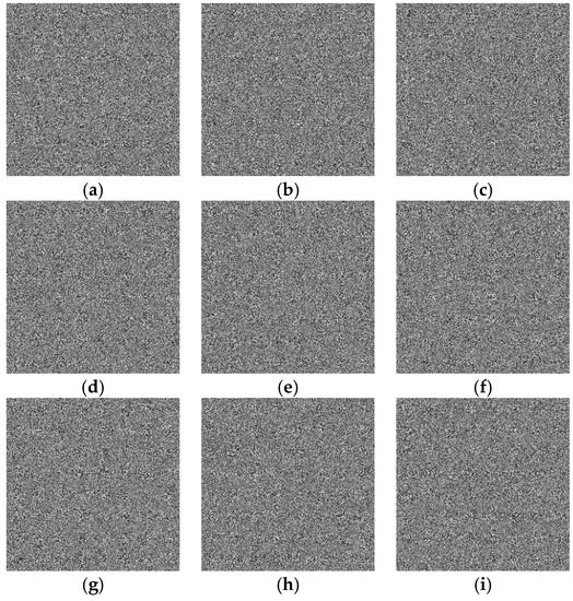
Figure 8. Encryption images of the proposed algorithm: (a) Image 1. (b) Image 2. (c) Image 3. (d) Image 4. (e) Image 5. (f) Image 6. (g) Image 7. (h) Image 8. (i) Image 9.

To encrypt the plain images in Figure 6 with Hua’s algorithm, we repeatedly performed the encryption process nine times. The encryption images are shown in Figure 9.

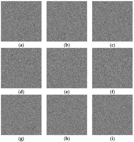
Figure 9. Encryption images of Hua’s algorithm: (a) Image 1. (b) Image 2. (c) Image 3. (d) Image 4. (e) Image 5. (f) Image 6. (g) Image 7. (h) Image 8. (i) Image 9.

To encrypt the plain images in Figure 6 with Wu’s algorithm, we repeatedly performed the encryption process nine times. The encryption images are shown in Figure 10.

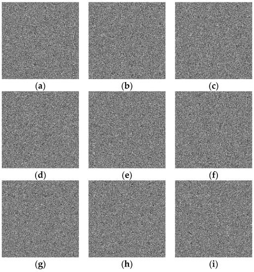
Figure 10. Encryption images of Wu’s algorithm: (a) Image 1. (b) Image 2. (c) Image 3. (d) Image 4. (e) Image 5. (f) Image 6. (g) Image 7. (h) Image 8. (i) Image 9.

To encrypt the plain images in Figure 6 with Li’s algorithm, Figure 11 is the reassembled image, which only contains the low-frequency coefficients of the plain images. Figure 12 is the encryption image. The decryption image is the same as Figure 11.

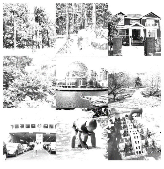
Figure 11. Reassembled image.

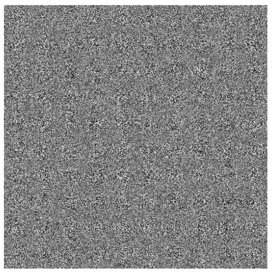
Figure 12. Encryption image of Li’s algorithm.

To encrypt the plain images in Figure 6 with Zhang’s Algorithm 1, Figure 13a–i are the encryption images. In this scenario, the size of the mixed image elements is $32\times 32$.

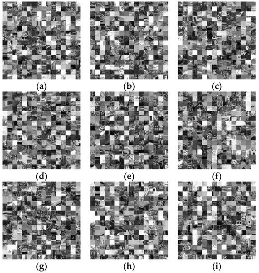
Figure 13. Encryption images of Zhang’s Algorithm 1: (a) Image 1. (b) Image 2. (c) Image 3. (d) Image 4. (e) Image 5. (f) Image 6. (g) Image 7. (h) Image 8. (i) Image 9.

To encrypt the plain images in Figure 6 with Zhang’s Algorithm 2, the encryption images are shown in Figure 14a–i.

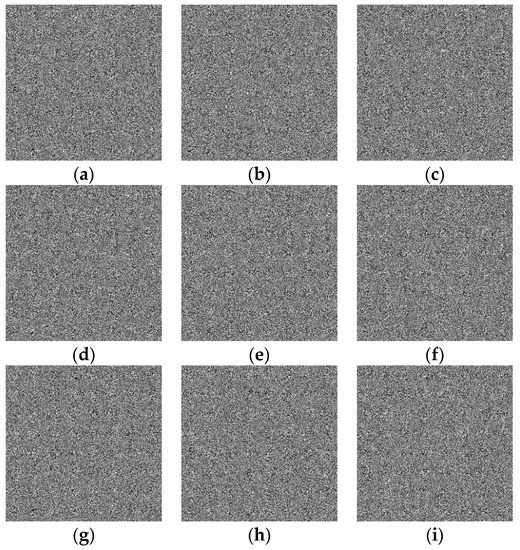
Figure 14. Encryption images of Zhang’s algorithm 2: (a) Image 1. (b) Image 2. (c) Image 3. (d) Image 4. (e) Image 5. (f) Image 6. (g) Image 7. (h) Image 8. (i) Image 9.

To encrypt the plain images in Figure 6 with Zhang’s Algorithm 3, the encryption images are shown in Figure 15a–i.

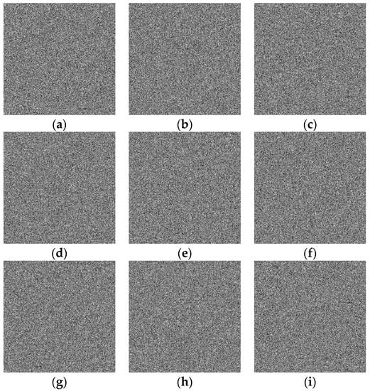
Figure 15. Encryption images of Zhang’s Algorithm 3: (a) Image 1. (b) Image 2. (c) Image 3. (d) Image 4. (e) Image 5. (f) Image 6. (g) Image 7. (h) Image 8. (i) Image 9.

To encrypt the plain images in Figure 6a,b with Suri’s algorithm, the encryption images are shown in Figure 16a,b.

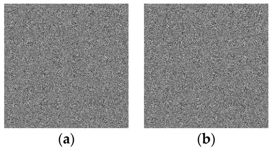
Figure 16. Encryption images of Suri’s algorithm: (a) Image 1. (b) Image 2.

To encrypt the plain images in Figure 6a,b with Das’s algorithm, the encryption images are shown in Figure 17a,b.

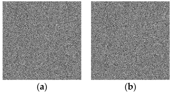
Figure 17. Encryption images of Das’s algorithm: (a) Image 1. (b) Image 2.

Therefore, the encryption images of Zhang’s Algorithm 1 stimulate the block effect for the large size of image blocks. The encryption image of Li’s algorithm is lossy and Bob can only recover the low-frequency coefficients of the plain images. However, the encryption images of the proposed algorithm, Hua’s algorithm, Wu’s algorithm, Li’s algorithm, Zhang’s Algorithms 2 and 3, Suri’s algorithm, and Das’s algorithm are very chaotic and have excellent encryption effects.

6. Algorithm Analyses

A desirable image encryption algorithm can resist several commonly used attacks. This paper discusses the performance of the proposed algorithm in detail.

6.1. Key Space Analysis

For the proposed algorithm, the keys are the variables $x_0,y_0,r_1,r_2,s_1,s_2$ of 2D Logistic map and the variables $z_0^1,z_0^2,p^1,p^2$ of two PWLCM systems. If the calculating precision is ${10}^{-16}$, the key space is ${10}^{160}$. For Hua’s algorithm, its key space is $2^{256}\approx 1.16\times {10}^{77}$. For Wu’s algorithm, its key space is ${10}^{128}$. Nevertheless, for Zhang’s Algorithms 1–3, Suri’s algorithm, and Das’s algorithm, their key spaces are ${10}^{16\times 4}={10}^{64}$. Lastly, the key spaces of all these algorithm are very large, but the proposed algorithm has the largest key space.

6.2. Histogram Analysis

Figure 18a–i are the histograms of plain images, respectively. They are different from each other and these histograms concentrate on some gray levels.

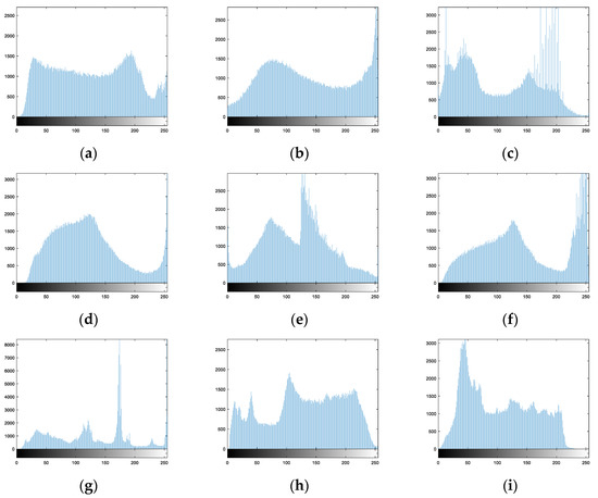
Figure 18. Histograms of plain images: (a) Image 1. (b) Image 2. (c) Image 3. (d) Image 4. (e) Image 5. (f) Image 6. (g) Image 7. (h) Image 8. (i) Image 9.

For the proposed algorithm, Figure 19a–i are the histograms of nine encryption images, respectively. They are similar to each other and the pixel number for the different gray levels is almost equal.

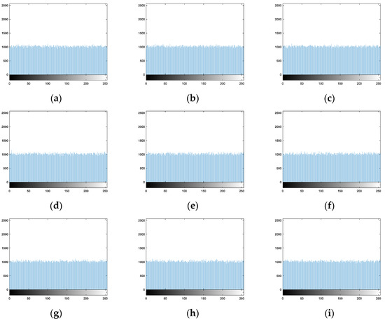
Figure 19. Histograms of encryption images of the proposed algorithm: (a) Image 1. (b) Image 2. (c) Image 3. (d) Image 4. (e) Image 5. (f) Image 6. (g) Image 7. (h) Image 8. (i) Image 9.

For Hua’s algorithm, Figure 20a–i are the histograms of nine encryption images, respectively. Hua’s algorithm not only scrambles the pixel positions but also changes the pixel values. Therefore, the histograms of encryption images are desirable.

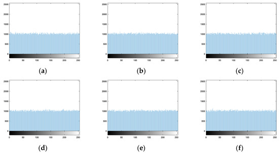
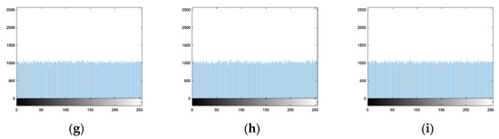
Figure 20. Histograms of encryption images of Hua’s algorithm: (a) Image 1. (b) Image 2. (c) Image 3. (d) Image 4. (e) Image 5. (f) Image 6. (g) Image 7. (h) Image 8. (i) Image 9.

For Wu’s algorithm, Figure 21a–i are the histograms of nine encryption images, respectively. Wu’s algorithm not only scrambles the pixel positions but also changes the pixel values. Therefore, the histograms of encryption images are desirable.

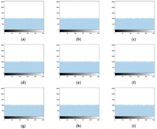
Figure 21. Histograms of encryption images of Wu’s algorithm: (a) Image 1. (b) Image 2. (c) Image 3. (d) Image 4. (e) Image 5. (f) Image 6. (g) Image 7. (h) Image 8. (i) Image 9.

For Zhang’s Algorithm 1, Figure 22a–i are the histograms of nine encryption images, respectively. Zhang’s Algorithm 1 only scrambles the pixel block positions. Therefore, the histograms of encryption images are undesirable.

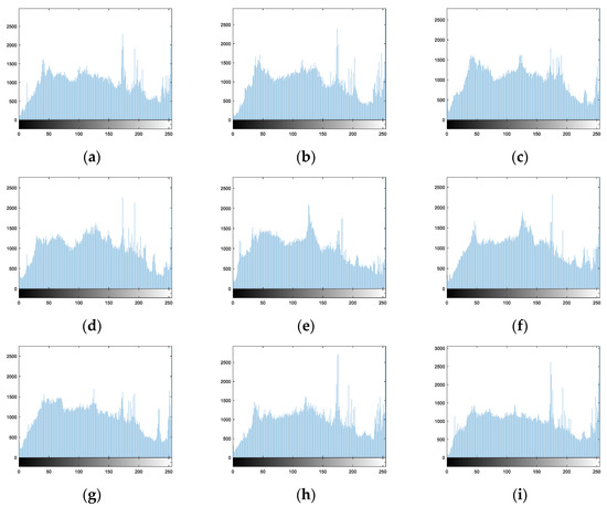
Figure 22. Histograms of encryption images of Zhang’s Algorithm 1: (a) Image 1. (b) Image 2. (c) Image 3. (d) Image 4. (e) Image 5. (f) Image 6. (g) Image 7. (h) Image 8. (i) Image 9.

For Zhang’s Algorithms 2 and 3 and Das’s algorithm, Figure 23a–i, Figure 24a–i, and Figure 25a,b are the histograms of their encryption images, respectively. These algorithms not only scramble the pixel positions but also change the pixel values. Therefore, these histograms are very uniform.

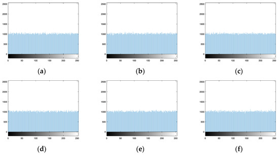
Figure 23. Histograms of encryption images of Zhang’s Algorithm 2: (a) Image 1. (b) Image 2. (c) Image 3. (d) Image 4. (e) Image 5. (f) Image 6. (g) Image 7. (h) Image 8. (i) Image 9.

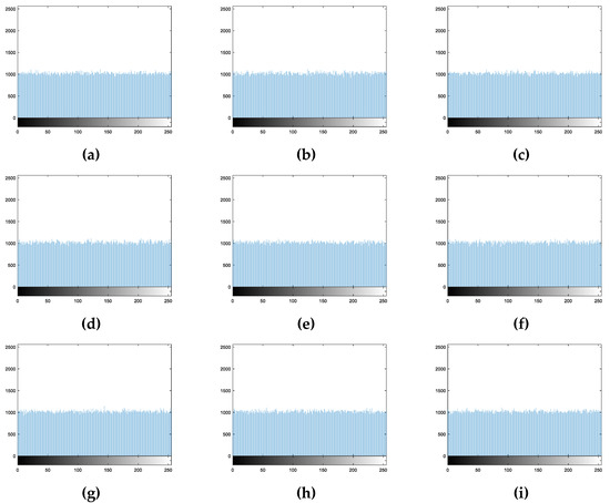
Figure 24. Histograms of encryption images of Zhang’s Algorithm 3: (a) Image 1. (b) Image 2. (c) Image 3. (d) Image 4. (e) Image 5. (f) Image 6. (g) Image 7. (h) Image 8. (i) Image 9.

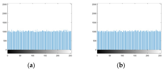
Figure 25. Histograms of encryption images of Das’s algorithm: (a) Image 1. (b) Image 2.

For Suri’s algorithm, Figure 26a,b are the histograms of encryption images, respectively. Equations (27) and (28) obviously reduce the pixel numbers for the lower gray levels and higher gray levels. Therefore, these histograms are not uniform.

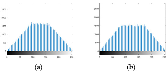
Figure 26. Histograms of encryption images of Suri’s algorithm: (a) Image 1. (b) Image 2.

Therefore, for Zhang’s Algorithm 1 and Suri’s algorithm, the histograms of their encryption images are not uniform. However, for the proposed algorithm, Hua’s algorithm, Wu’s algorithm, Zhang’s Algorithms 2 and 3, and Das’s algorithm, the histograms of their encryption images are desirable, which are very different from the histograms in Figure 18.

6.3. Correlation Analysis

The correlation coefficient of adjacent pixels is defined by the equations below.

$$r_{x,y}=\frac{E\left(\left(x-E\left(x\right)\right)\left(y-E\left(y\right)\right)\right)}{\sqrt{D\left(x\right)D\left(y\right)}},$$

(29)

$$E\left(x\right)=\frac{1}{N}{\displaystyle \sum _{\mathrm{i}=1}^N{x}_i},$$

(30)

$$D\left(x\right)=\frac{1}{N}{\displaystyle \sum _{i=1}^N{\left(x_i-E\left(x\right)\right)}^2},$$

(31)

where $E(•),D(•)$ denote the expectation and variance, respectively.

For the proposed algorithm, we take the first plain image and encryption image as examples to evaluate the performance of pixel correlation. We select randomly 5000 pixels from them and obtain their adjacent pixels. Figure 27 and Figure 28 reflect their correlation. From Figure 27, we can see that the pixel correlation of the plain image is very strong. Figure 28 is very chaotic and shows that the pixel correlation of the encryption image is very weak.

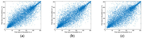
Figure 27. Adjacent pixel correlation of the first plain image: (a) Horizontal direction. (b) Vertical direction. (c) Diagonal direction.

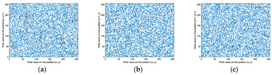
Figure 28. Adjacent pixel correlation of the first encryption image: (a) Horizontal direction. (b) Vertical direction. (c) Diagonal direction.

Table 1 shows the correlation coefficients of plain images. For the proposed algorithm, Hua’s algorithm, Wu’s algorithm, Li’s algorithm, and Zhang’s Algorithms 1–3, Suri’s algorithm, and Das’s algorithm, the correlation coefficients are listed in Table 2. The data in Table 1 display that the correlation coefficients are very large. However, the data in Table 2 display that the correlation coefficients are very small for the proposed algorithm, Hua’s algorithm, Wu’s algorithm, Zhang’s Algorithms 2 and 3, Suri’s algorithm, and Das’s algorithm. However, for Zhang’s Algorithm 1, the correlation coefficients in Table 2 are very large. Therefore, the proposed algorithm destroys the pixel correlation well.

Table 1. Correlation coefficients of plain images.

Directions	Horizontal	Vertical	Diagonal
Plain image 1	0.8788	0.8733	0.8256
Plain image 2	0.9239	0.9170	0.8779
Plain image 3	0.9395	0.9131	0.8820
Plain image 4	0.9440	0.9353	0.9032
Plain image 5	0.8841	0.8178	0.7632
Plain image 6	0.9504	0.9422	0.9165
Plain image 7	0.9896	0.9848	0.9751
Plain image 8	0.9812	0.9666	0.9528
Plain image 9	0.9603	0.9579	0.9265

Table 2. Correlation coefficients of encryption images.

Algorithms	Names	Horizontal	Vertical	Diagonal
Hua’s algorithm	Encryption image 1	0.0011	−0.0019	−0.0084
	Encryption image 2	−0.0012	0.0013	0.0016
	Encryption image 3	0.0019	0.0044	0.0020
	Encryption image 4	0.0016	0.0039	−0.0022
	Encryption image 5	−0.0056	−0.0013	−0.0033
	Encryption image 6	−0.0063	−0.0007	−0.0006
	Encryption image 7	0.0006	−0.0004	−0.0002
	Encryption image 8	−0.0010	0.0007	0.0001
	Encryption image 9	0.0012	−0.0011	−0.0015
Wu’s algorithm	Encryption image 1	0.0034	−0.0022	0.0014
	Encryption image 2	0.0011	−0.0037	0.0014
	Encryption image 3	0.0024	0.0002	0.0017
	Encryption image 4	0.0012	0.0012	−0.0059
	Encryption image 5	0.0007	0.0049	−0.0035
	Encryption image 6	0.0014	0.0015	−0.0023
	Encryption image 7	0.0007	0.0034	0.0017
	Encryption image 8	0.0009	0.0025	−0.0027
	Encryption image 9	0.0025	−0.0026	−0.0007
The proposed algorithm	Encryption image 1	0.0021	0.0013	−0.0024
	Encryption image 2	−0.0047	0.0147	0.0014
	Encryption image 3	0.0016	0.0026	0.0001
	Encryption image 4	0.0012	−0.0001	0.0033
	Encryption image 5	−0.0022	0.0018	0.0021
	Encryption image 6	−0.0021	−0.0026	0.0018
	Encryption image 7	−0.0043	−0.0034	0.0030
	Encryption image 8	−0.0020	0.0026	−0.0001
	Encryption image 9	0.0024	0.0001	−0.0028
Zhang’s Algorithm 1	Encryption image 1	0.9463	0.9356	0.8806
	Encryption image 2	0.9469	0.9345	0.8803
	Encryption image 3	0.9454	0.9283	0.8745
	Encryption image 4	0.9422	0.9251	0.8695
	Encryption image 5	0.9367	0.9209	0.8607
	Encryption image 6	0.9395	0.9275	0.8701
	Encryption image 7	0.9408	0.9236	0.8643
	Encryption image 8	0.9492	0.9409	0.8875
	Encryption image 9	0.9491	0.9367	0.8849
Zhang’s Algorithm 2	Encryption image 1	−0.0045	−0.0001	−0.0047
	Encryption image 2	−0.0090	−0.0039	0.0005
	Encryption image 3	−0.0070	−0.0003	−0.0006
	Encryption image 4	−0.0046	0.0001	−0.0023
	Encryption image 5	−0.0092	0.0005	−0.0024
	Encryption image 6	−0.0099	0.0010	−0.0047
	Encryption image 7	−0.0051	−0.0007	−0.0030
	Encryption image 8	−0.0109	−0.0009	−0.0042
	Encryption image 9	−0.0099	−0.0010	0.0020
Zhang’s Algorithm 3	Encryption image 1	−0.0004	−0.0001	0.0006
	Encryption image 2	−0.0004	−0.0002	−0.0027
	Encryption image 3	0.0012	0	0.0020
	Encryption image 4	−0.0048	−0.0020	0.0027
	Encryption image 5	0.0006	0.0011	−0.0069
	Encryption image 6	−0.0016	0.0019	−0.0006
	Encryption image 7	−0.0002	0.0014	0.0003
	Encryption image 8	−0.0012	0.0018	0.0018
	Encryption image 9	0.0037	−0.0012	0.0011
Suri’s algorithm	Encryption image 1	0	−0.0015	−0.0023
	Encryption image 2	−0.0044	−0.0025	0.0005
Das’s algorithm	Encryption image 1	−0.0037	−0.0015	0.0041
	Encryption image 2	−0.0059	−0.0022	−0.0011

6.4. Differential Attack Analysis

The differential attack can check the plaintext sensitivity for an image encryption algorithm [26]. Therefore, for a little change to the plain image, an excellent image encryption algorithm can spread this influence over the whole encryption process. The Number of Pixels Change Rate (NPCR) is shown below.

$$f\left(i,j\right)=\{\begin{array}{l}\begin{array}{cc}0& I^{\prime }\left(i,j\right)=I^{″}\left(i,j\right)\end{array}\\ \begin{array}{cc}1& I^{\prime }\left(i,j\right)\ne I^{″}\left(i,j\right)\end{array}\end{array},$$

(32)

$$NPCR=\frac{{\displaystyle \sum _{i=1}^m{\displaystyle \sum _{j=1}^{n}f\left(i,j\right)}}}{m\times n}\times 100\%,$$

(33)

where $I^{\prime }\left(i,j\right)$ and $I^{″}\left(i,j\right)$ denote two encrypted images. One corresponds to the plain image while the other corresponds to the changed plain image.

The Unified Average Changing Intensity (UACI) is shown in the equation below.

$$UACI=\frac{{\displaystyle \sum _{i=1}^m{\displaystyle \sum _{j=1}^n\left|I^{\prime }\left(i,j\right)-I^{″}\left(i,j\right)\right|}}}{255\times m\times n}\times 100\%.$$

(34)

Even if two images are very similar, their hash values of SHA-256 are completely different [27]. We changed the gray value of $I^1(1,1)$ from the original value 59 into 200. For the proposed algorithm, Hua’s algorithm, Wu’s algorithm, Zhang’s Algorithms 1–3, Suri’s algorithm, and Das’s algorithm, experimental data are shown in Table 3. For Hua’s algorithm and Wu’s algorithm, we list the NPCR and UACI values of the plain image 1. For the proposed algorithm, Hua’s algorithm, Wu’s algorithm, and Zhang’s Algorithms 2 and 3, the NPCR and UACI values are very large. For Suri’s algorithm, the UACI values are a little smaller. However, the NPCR and UACI values are zero for Zhang’s Algorithm 1 and Das’s algorithm. Therefore, the proposed algorithm is strong for the differential attack.

Table 3. NPCR and UACI values.

Algorithms	Name	NPCR	UACI
Hua’s algorithm	Plain image 1	99.60%	33.43%
Wu’s algorithm	Plain image 1	99.99%	33.61%
The proposed algorithm	Plain image 1	99.64%	33.55%
	Plain image 2	99.63%	33.61%
	Plain image 3	99.68%	33.72%
	Plain image 4	99.68%	33.71%
	Plain image 5	99.63%	33.70%
	Plain image 6	99.67%	33.60%
	Plain image 7	99.67%	33.63%
	Plain image 8	99.65%	33.65%
	Plain image 9	99.65%	33.71%
Zhang’s Algorithm 1	Plain image 1	0	0
	Plain image 2	0	0
	Plain image 3	0	0
	Plain image 4	0	0
	Plain image 5	0	0
	Plain image 6	0	0
	Plain image 7	0	0
	Plain image 8	0	0
	Plain image 9	0	0
Zhang’s Algorithm 2	Plain image 1	99.64%	33.55%
	Plain image 2	99.63%	33.61%
	Plain image 3	99.68%	33.72%
	Plain image 4	99.68%	33.71%
	Plain image 5	99.63%	33.70%
	Plain image 6	99.67%	33.60%
	Plain image 7	99.67%	33.63%
	Plain image 8	99.65%	33.65%
	Plain image 9	99.65%	33.71%
Zhang’s Algorithm 3	Plain image 1	99.61%	33.51%
	Plain image 2	99.62%	33.47%
	Plain image 3	99.59%	33.47%
	Plain image 4	99.61%	33.48%
	Plain image 5	99.61%	33.47%
	Plain image 6	99.62%	33.52%
	Plain image 7	99.62%	33.48%
	Plain image 8	99.62%	33.44%
	Plain image 9	99.63%	33.51%
Suri’s algorithm	Plain image 1	99.33%	21.066%
	Plain image 2	98.79%	10.07%
Das’s algorithm	Plain image 1	0	0
	Plain image 2	0	0

6.5. Information Entropy Analysis

For the gray image $I$, we define the information entropy by the equation below.

$$H\left(I\right)=-{\displaystyle \sum _{i=0}^{255}P\left(m_i\right){\log }_{2}P\left(m_i\right)},$$

(35)

where $m_i$, $i=0,1,\cdots ,255$ represents the $i$th gray level and $P\left(m_i\right)$ denotes the emergence probability. For the proposed algorithm, Hua’s algorithm, Wu’s algorithm, Zhang’s Algorithms 1–3, Suri’s algorithm, and Das’s algorithm, the entropy values of encrypted images are shown in Table 4. For Hua’s algorithm and Wu’s algorithm, we list the entropy values of the encryption image 1. For Zhang’s Algorithm 1 and Suri’s algorithm, their values are smaller than the values of the proposed algorithm. Nevertheless, for the proposed algorithm, Hua’s algorithm, Wu’s algorithm, Zhang’s Algorithms 2 and 3, Suri’s algorithm, and Das’s algorithm, the entropy values are very large, which means these algorithms are strong for the statistical attack.

Table 4. Information entropy values.

Algorithms	Names	Entropy
Hua’s algorithm	Encryption image 1	7.9992
Wu’s algorithm	Encryption image 1	7.9993
The proposed algorithm	Encryption image 1	7.9993
	Encryption image 2	7.9993
	Encryption image 3	7.9994
	Encryption image 4	7.9992
	Encryption image 5	7.9992
	Encryption image 6	7.9992
	Encryption image 7	7.9993
	Encryption image 8	7.9993
	Encryption image 9	7.9994
Zhang’s Algorithm 1	Encryption image 1	7.8442
	Encryption image 2	7.8339
	Encryption image 3	7.8817
	Encryption image 4	7.8827
	Encryption image 5	7.8819
	Encryption image 6	7.8951
	Encryption image 7	7.8912
	Encryption image 8	7.8534
	Encryption image 9	7.8312
Zhang’s Algorithm 2	Encryption image 1	7.9993
	Encryption image 2	7.9993
	Encryption image 3	7.9994
	Encryption image 4	7.9994
	Encryption image 5	7.9993
	Encryption image 6	7.9993
	Encryption image 7	7.9993
	Encryption image 8	7.9992
	Encryption image 9	7.9992
Zhang’s Algorithm 3	Encryption image 1	7.9994
	Encryption image 2	7.9992
	Encryption image 3	7.9994
	Encryption image 4	7.9992
	Encryption image 5	7.9993
	Encryption image 6	7.9992
	Encryption image 7	7.9994
	Encryption image 8	7.9994
	Encryption image 9	7.9994
Suri’s algorithm	Encryption image 1	7.7558
	Encryption image 2	7.7825
Das’s algorithm	Encryption image 1	7.9992
	Encryption image 2	7.9992

6.6. Lossy Analysis

The lossless image encryption algorithm is expected in most cases. For Li’s algorithm, the decryption image is lossy, which only contains the low-frequency coefficients of plain images. For Suri’s algorithm, the weights in Equations (27) and (28) are decimals. Therefore, the decryption images are slightly lossy. However, for the proposed algorithm, Hua’s algorithm, Wu’s algorithm, Zhang’s Algorithms 1–3, and Das’s algorithm, the decryption images are lossless.

6.7. Input Image Number Analysis

As an MIE algorithm, the input image number is expected to be suitable for many cases. For Hua’s algorithm and Wu’s algorithm, they can only encrypt one plain image at once. For Suri’s algorithm and Das’s algorithm, they can only encrypt two plain images at once. However, for the proposed algorithm, Li’s algorithm, and Zhang’s Algorithms 1–3, they can encrypt $k$ plain images at once and their input image number can be determined by the user. Therefore, the superiority of the proposed algorithm is over both Suri’s algorithm and Das’s algorithm.

6.8. Time Complexity Analysis

(1) Computation Complexity Analysis

The size of $k$ plain images is $m\times n$. The computation complexity for adjusting a pixel, a DNA code, a bit, or an image block position, DNA coding a pixel, the decimal-binary conversion on a pixel, and XOR or DNA XOR operation on a pixel value, DWT on a pixel, Arnold transformation on a pixel, and AES encrypting a pixel is $S,D,B,X,W,A$, and $E$ on average, respectively.

(1) For the proposed algorithm, the main time-consuming operations include scrambling the pixel position with the 3D permutation model and the XOR operation for changing the pixel values. For the permutation with the internal-row mode, all the pixel positions of $k$ plain images are scrambled, which means the computation complexity is $k\times m\times n\times S$. Similarly, the computation complexity of both the internal-column and external modes is $k\times m\times n\times S$. For the image diffusion stage, all the pixel values of $k$ plain images are performed by the XOR with the chaotic image $C^2$. Therefore, the computation complexity is $k\times m\times n\times X$. Lastly, the computation complexity for the proposed algorithm is about $kmn(3S+X)$ in total.

(2) For Hua’s algorithm, the main time-consuming operations include scrambling the pixel positions and changing the pixel values. The computation complexity for changing a pixel value is $Q$ on average with Equation (20). To encrypt one plain image, we need to perform four rounds of permutation and diffusion operations. Therefore, to encrypt $k$ plain images, the computation complexity for Hua’s algorithm is about $4kmn(S+Q)$.

(3) For Wu’s algorithm, the main time-consuming operations are the DNA coding, scrambling DNA codes, XOR operation, and the DNA XOR operation. To encrypt one plain image, we need to encode $R,P$ and decode $DN{A}_{P1}$ with the DNA coding theory. At the same time, we need to perform the DNA XOR operation and XOR operation in Equations (25) and (26), respectively. Therefore, to encrypt $k$ plain images, the computation complexity for Wu’s algorithm is about $kmn(3D+2X)$.

(4) For Li’s algorithm, the main time-consuming operations are the DWT transformation, the Arnold transformation, and the XOR operation. All the pixel values of $k$ plain images are performed by the DWT operation. Therefore, the computation complexity is $k\times m\times n\times W$. The reassembled image only constituted of low-frequency coefficients is scrambled with the Arnold transformation. Therefore, the computation complexity is $\frac{1}{4}\times k\times m\times n\times A$. All the pixel values of $k$ plain images are performed by the XOR with the chaotic image. Therefore, the computation complexity is $\frac{1}{4}\times k\times m\times n\times X$. Lastly, the computation complexity for Li’s algorithm is about $\frac{kmn}{4}(4W+A+X)$ in total.

(5) For Zhang’s Algorithm 1, the main time-consuming operation is scrambling image blocks. If the size of image blocks are $8\times 8$, there are $\frac{1}{64}\times k\times m\times n$ image blocks for $k$ plain images. Therefore, the computation complexity for Zhang’s Algorithm 1 is about $\frac{kmnS}{64}$.

(6) For Zhang’s Algorithm 2, the main time-consuming operations are the scrambling of the image blocks and the XOR operation. If the size of image blocks is $8\times 8$, the computation complexity of scrambling the image blocks is $\frac{kmnS}{64}$. The computation complexity of the XOR operation is $k\times m\times n\times X$. Lastly, the computation complexity for Zhang’s Algorithm 2 is about $kmn\left(\frac{S}{64}+X\right)$ in total.

(7) For Zhang’s Algorithm 3, the main time-consuming operations are the DNA coding, scrambling DNA codes, and the DNA XOR operation. The computation complexity for Zhang’s Algorithm 3 is about $mn\left[k\left(2D+S+X\right)+D\right]$ in total [19].

(8) For Suri’s algorithm, the main time-consuming operations are the XOR operation and AES encryption. The computation complexity for Suri’s algorithm is about $mn\left(X+E\right)$.

(9) For Das’s algorithm, the main time-consuming operations are the decimal-binary conversion, scrambling bits between the pixel values, and the XOR operation. The computation complexity for Das’s algorithm is about $2mn\left(2B+S+X\right)$.

(2) Encryption Time Analysis

To encrypt the plain images in Figure 6, this paper implements the proposed algorithm, Hua’s algorithm, Wu’s algorithm, Li’s algorithm, Zhang’s Algorithms 1–3, Suri’s algorithm, and Das’s algorithm with Matlab R2016a. The hardware environment is PC with Intel M-5Y71@1.20 GHz CPU and 8 GB Memory. The encryption time of these image algorithms is listed in Table 5. The experimental results show that the encryption speed of Zhang’s Algorithm 1 is the fastest and the proposed algorithm is faster than Hua’s algorithm, Wu’s algorithm, Li’s algorithm, Zhang’s Algorithm 3, Suri’s algorithm, or Das’s algorithm. Therefore, the proposed algorithm is the most efficient, which is suitable for practical image encryption.

Table 5. Encryption time (unit: second).

Algorithms	Time
The proposed algorithm	8.7202
Hua’s algorithm	21.4147
Wu’s algorithm	1300.484
Li’s algorithm	85.1965
Zhang’s algorithm 1	0.255 [17]
Zhang’s algorithm 2	0.7103 [18]
Zhang’s algorithm 3	43 [20]
Suri’s algorithm	407.9352
Das’s algorithm	149.7175

7. Conclusions and Outlook

Inspired by the magic cube game, this paper establishes a 3D permutation model to permute images, which includes the internal-row, internal-column, and external modes. An MIE algorithm is designed with the 3D permutation model. When compared with eight similar algorithms, the proposed algorithm performs well. Simulation and algorithm evaluation display that the proposed algorithm is secure and efficient.

References

- Wang, X.; Zhu, X.; Wu, X.; Zhang, Y. Image encryption algorithm based on multiple mixed hash functions and cyclic shift. Opt. Lasers Eng. 2018, 107, 370–379. [Google Scholar] [CrossRef]
- Chai, X.; Zheng, X.; Gan, Z.; Han, D.; Chen, Y. An image encryption algorithm based on chaotic system and compressive sensing. Signal Process. 2018, 148, 124–144. [Google Scholar] [CrossRef]
- Wu, X.; Wang, K.; Wang, X.; Kan, H.; Kurthsef, J. Color image DNA encryption using NCA map-based CML and one-time keys. Signal Process. 2018, 148, 272–287. [Google Scholar] [CrossRef]
- Gan, Z.; Chai, X.; Yuan, K.; Lu, Y. A novel image encryption algorithm based on LFT based S-boxes and chaos. Multimed. Tools Appl. 2018, 77, 8759–8783. [Google Scholar] [CrossRef]
- Ahmad, M.; Al Solami, E.; Wang, X.-Y.; Doja, M.N.; Sufyan Beg, M.M.; Alzaidi, A.A. Cryptanalysis of an image encryption algorithm based on combined chaos for a BAN system, and improved scheme using SHA-512 and hyperchaos. Symmetry 2018, 10, 266. [Google Scholar] [CrossRef]
- Bashir, Z.; Watróbski, J.; Rashid, T.; Zafar, S.; Sałabun, W. Chaotic dynamical state variables selection procedure based image encryption scheme. Symmetry 2017, 9, 312. [Google Scholar] [CrossRef]
- Hua, Z.; Jin, F.; Xu, B.; Wang, H. 2D Logistic-Sine-coupling map for image encryption. Signal Process. 2018, 149, 148–161. [Google Scholar] [CrossRef]
- Wu, J.; Liao, X.; Yang, B. Image encryption using 2D Hénon-Sine map and DNA approach. Signal Process. 2018, 153, 11–23. [Google Scholar] [CrossRef]
- Liu, W.; Xie, Z.; Liu, Z.; Zhang, Y.; Liu, S. Multiple-image encryption based on optical asymmetric key cryptosystem. Opt. Commun. 2015, 335, 205–211. [Google Scholar] [CrossRef]
- Di, H.; Kang, Y.; Liu, Y.; Zhang, X. Multiple image encryption by phase retrieval. Opt. Eng. 2016, 55, 1–7. [Google Scholar] [CrossRef]
- Xiong, Y.; Quan, C.; Tay, C.J. Multiple image encryption scheme based on pixel exchange operation and vector decomposition. Opt. Lasers Eng. 2018, 101, 113–121. [Google Scholar] [CrossRef]
- Zhang, L.; Zhou, Y.; Huo, D.; Li, J.; Zhou, X. Multiple-image encryption based on double random phase encoding and compressive sensing by using a measurement array preprocessed with orthogonal-basis matrices. Opt. Laser Technol. 2018, 105, 162–170. [Google Scholar] [CrossRef]
- Li, X.; Meng, X.; Yang, X.; Wang, Y.; Yin, Y.; Peng, X.; He, W.; Dong, G.; Chen, H. Multiple-image encryption via lifting wavelet transform and XOR operation based on compressive ghost imaging scheme. Opt. Lasers Eng. 2018, 102, 106–111. [Google Scholar] [CrossRef]
- Deng, P.; Diao, M.; Shan, M.; Zhong, Z.; Zhang, Y. Multiple-image encryption using spectral cropping and spatial multiplexing. Opt. Commun. 2018, 359, 234–239. [Google Scholar] [CrossRef]
- Yuan, S.; Liu, X.; Zhou, X.; Li, Z. Multiple-image encryption scheme with a single-pixel detector. J. Mod. Opt. 2016, 63, 1457–1465. [Google Scholar] [CrossRef]
- Li, C.-L.; Li, H.-M.; Li, F.-D.; Wei, D.-Q.; Yang, X.-B.; Zhang, J. Multiple-image encryption by using robust chaotic map in wavelet transform domain. Optik 2018, 171, 277–286. [Google Scholar] [CrossRef]
- Zhang, X.; Wang, X. Multiple-image encryption algorithm based on mixed image element and chaos. Comput. Electr. Eng. 2017, 11, 1–13. [Google Scholar] [CrossRef]
- Zhang, X.; Wang, X. Multiple-image encryption algorithm based on mixed image element and permutation. Opt. Lasers Eng. 2017, 92, 6–16. [Google Scholar] [CrossRef]
- Zhang, X.; Wang, X. Multiple-image encryption algorithm based on DNA encoding and chaotic system. Multimed. Tools Appl. 2018, 67, 1–29. [Google Scholar] [CrossRef]
- Shelza, S.; Ritu, V. An AES-chaos-based hybrid approach to encrypt multiple images. Adv. Intell. Syst. Comput. 2017, 555, 37–43. [Google Scholar] [CrossRef]
- Subhajit, D.; SatyendraNath, M.; Nabin, G. Multiple-image encryption using genetic algorithm. Adv. Intell. Syst. Comput. 2015, 343, 145–153. [Google Scholar] [CrossRef]
- Wikipedia. Rubik’s Cube. Available online: https://en.wikipedia.org/wiki/Rubik%27s_Cube (accessed on 24 July 2018).
- Zhang, X.; Zhu, G.; Ma, S. Remote-sensing image encryption in hybrid domains. Opt. Commun. 2012, 285, 1736–1743. [Google Scholar] [CrossRef]
- Wang, X.; Xu, D. A novel image encryption scheme based on Brownian motion and PWLCM chaotic system. Nonlinear Dyn. 2015, 75, 345–353. [Google Scholar] [CrossRef]
- Guesmi, R.; Farah, M.A.B.; Kachouri, A.; Samet, M. A novel chaos-based image encryption using DNA sequence operation and Secure Hash Algorithm SHA-2. Nonlinear Dyn. 2015, 83, 1123–1136. [Google Scholar] [CrossRef]
- Belazi, A.; El-Latif, A.A.A.; Belghith, S. A novel image encryption scheme based on substitution-permutation network and chaos. Signal Process. 2016, 128, 155–170. [Google Scholar] [CrossRef]
- Chai, X.; Chen, Y.; Broyde, L. A novel chaos-based image encryption algorithm using DNA sequence operations. Opt. Lasers Eng. 2017, 88, 197–213. [Google Scholar] [CrossRef]
© 2018 by the authors. Licensee MDPI, Basel, Switzerland. This article is an open access article distributed under the terms and conditions of the Creative Commons Attribution (CC BY) license (http://creativecommons.org/licenses/by/4.0/).