A New Radar Signal Recognition Method Based on Optimal Classification Atom and IDCQGA

Abstract

Radar electronic reconnaissance is an important part of modern and future electronic warfare systems and is the primary method to obtain non-cooperative intelligence information. As the task requirement of radar electronic reconnaissance, it is necessary to identify the non-cooperative signals from the mixed signals. However, with the complexity of battlefield electromagnetic environment, the performance of traditional recognition system is seriously affected. In this paper, a new recognition method based on optimal classification atom and improved double chains quantum genetic algorithm (IDCQGA) is researched, optimal classification atom is a new feature for radar signal recognition, IDCQGA with symmetric coding performance can be applied to the global optimization algorithm. The main contributions of this paper are as follows: Firstly, in order to measure the difference of multi-class signals, signal separation degree based on distance criterion is proposed and established according to the inter-class separability and intra-class aggregation of the signals. Then, an IDCQGA is proposed to select the best atom for classification under the constraint of distance criterion, and the inner product of the signal and the best atom for classification is taken as the eigenvector. Finally, the extreme learning machine (ELM) is introduced as classifier to complete the recognition of signals. Simulation results show that the proposed method can improve the recognition rate of multi-class signals and has better processing ability for overlapping eigenvector parameters.

1. Introduction

Signal recognition is one of the main research directions in the field of electronic reconnaissance [1,2]. Fast and accurate identification of enemy signals can grasp advantages in battlefield environment perception, information control, and operational command, which has an important impact on the trend of war. Nowadays, radar signals have the characteristics of changeable intra-pulse modulation. It is a reliable way to improve the recognition ability of radar signals to study the extraction of intra-pulse features. The intra-pulse modulation of radar signals can be divided into intentional modulation and unintentional modulation [3]. Intentional modulation is an artificial modulation mode to improve the detection performance and resist enemy reconnaissance. Unintentional modulation refers to inherent parameter differences of radar equipment. This paper mainly studies the recognition of intentional modulation, which consists of feature extraction and classifier design. Feature extraction is equivalent to transforming radar signals from high-dimensional signal space to low-dimensional feature space, while classification or recognition are equivalent to transforming from feature space to decision space.

For feature extraction, delay autocorrelation and phase difference characteristics, instantaneous characteristics, statistical characteristics, and transform domain characteristics are the most widely used [4]. The delay autocorrelation and phase difference between different modulation types can effectively identify the phase modulation signal by comparing the periodic differences of waveforms [5]. Instantaneous characteristics, such as instantaneous amplitude, instantaneous frequency and instantaneous phase, can clearly express the changing rules of non-stationary signals [6]. Statistical features have good noise adaptability. By calculating the different order statistics, cumulative tensor, cyclostationary characteristics of the signal, the noise can be filtered out and the difference between the statistics can be applied to identify the signal [7]. Transform domain feature is easier to express details by means of spectral analysis in the transform domain, such as time-frequency (TF) analysis and atom matching [8,9]. Sparse decomposition and representation is a frontier feature extraction method in atom matching. At present, the most commonly applied sparse decomposition methods are matching pursuit (MP), orthogonal matching pursuit (OMP), stagewise orthogonal matching pursuit (StOMP), adaptive matching pursuit (SAMP), regularized orthogonal matching pursuit (ROMP), compressed sampling matching pursuit (CoSaMP) and so on [10,11,12,13,14,15]. OMP algorithm and its variants are the theoretic basis, and they have become the focus of researchers [16].

In addition, in order to increase the matching speed of OMP algorithm, researchers usually combine OMP with artificial intelligence methods to search the optimal atoms [17,18,19]. The artificial intelligence search algorithm is an efficient global optimization method, which has strong universality and adaptability for parallel processing. In sparse decomposition, genetic algorithm (GA) [20,21] and quantum genetic algorithm (QGA) [22,23] et al. are commonly used. QGA is a new intelligent search algorithm, which combines GA and quantum information theory to complete global optimization. As a branch of the QGA, double chains quantum genetic algorithm (DCQGA) has been one of the burning research problems in recent years, because of its small population size, strong searching ability and fast convergence speed [24,25]. However, the DCQGA has its own shortcomings: first of all, DCQGA with large encoding space range affects the convergence rate; secondly, the chromosome mutation is treated by the NOT-gate, but it usually cannot achieve the purpose of increasing the population diversity.

For classifier design, the existing methods can be divided into three categories: Bayesian decision-based classifier, pattern recognition-based classifier and neural network-based classifier [26]. Decision tree is a classification system composed of multistage classifiers. Using decision tree, the original complex multi-classification problem can be transformed into several dichotomy problems. By solving the dichotomy problem layer by layer, the multi-classification problem can be solved eventually. However, with more and more types of radar waveforms, the classification process of decision tree theory also increases, and the decision tree becomes more and more complex. Pattern recognition theory and artificial neural network can effectively solve these problems [27,28]. Taking the support vector machine (SVM) and extreme learning machine (ELM) classifiers as example, SVM and ELM construct feature space according to feature dimension, and establish classification hyperplane between features of different categories [29,30]. The hyperplane is the result of feature vector synthesis of all dimensions. No matter how complex the dimension of the input vector and the number of the output classification results are, only a few steps of calculation are needed to obtain a better recognition success rate than the decision tree.

By analyzing the above method, we find that there are three problems in atom matching for feature extraction. Firstly, the optimal matching atom obtained by the traditional OMP algorithm is only the optimal matching of the signal, and the relationship between the intra-class distance and the inter-class distance of different signals is not considered in the matching process. In other words, the atoms matched are the optimal matches for this signal but may not be the optimal classification atoms for several types of signals. Secondly, both of the training signal and the test signal need to be decomposed in the over-complete atom library, which greatly increases the computational complexity. Thirdly, more excellent DCQGA needs to be proposed to improve the convergence speed of OMP algorithm.

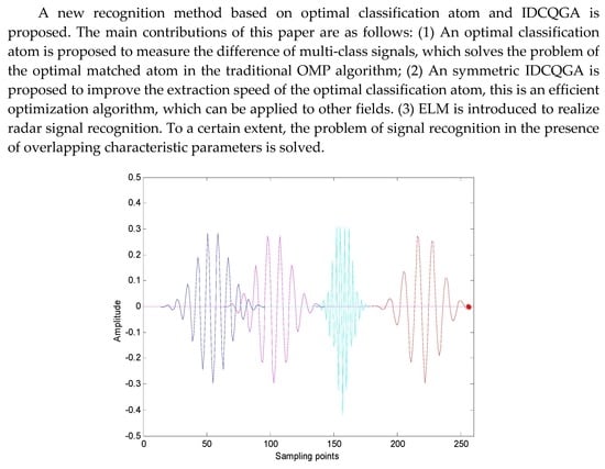
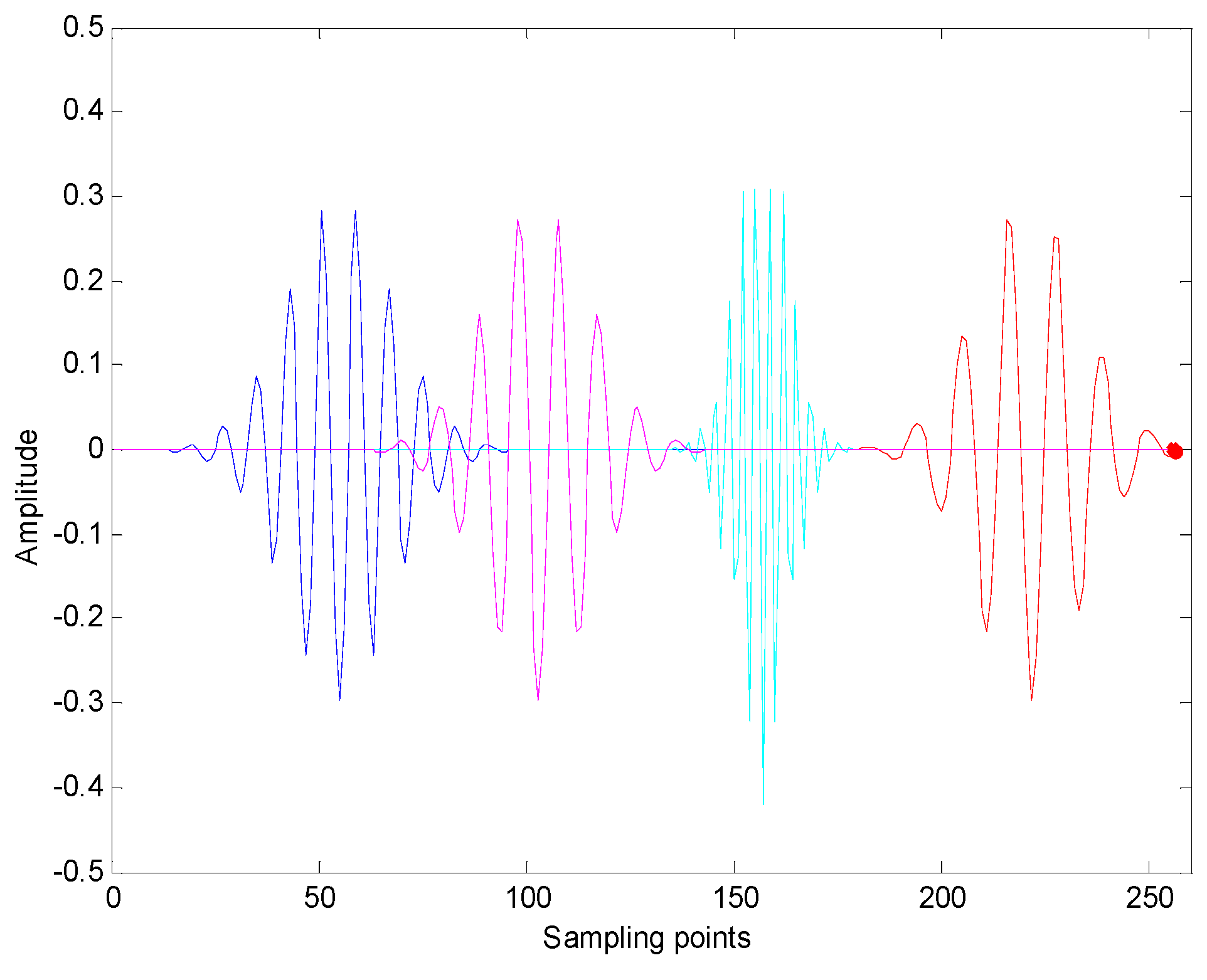
In order to solve these three problems, this paper proposes an optimal classification atom feature extraction and recognition method based on distance criterion. Firstly, the concept of signal separation degree based on distance criterion is established according to the inter-class separability and intra-class aggregation. Then, the improved double-stranded quantum genetic algorithm (IDCQGA) is applied to select the optimal atoms suitable for classification, and the inner product of each reconnaissance signal and the extracted atoms is used as the eigenvector. Finally, the signal classification and recognition is realized by the extreme learning machine (ELM). The main contributions of this paper are as follows: (1) Under the constraint of distance criterion, an optimal classification atom is proposed to measure the difference of multi-class signals, which is inspired by the traditional OMP algorithm; (2) An IDCQGA is proposed to improve the extraction speed of the optimal classification atom, this is an efficient optimization algorithm, which can be applied to other fields. (3) ELM is introduced to realize radar signal recognition. To a certain extent, the problem of signal recognition in the presence of overlapping characteristic parameters is solved.

The rest of this paper is organized as follows. Section 2 introduces the model and traditional algorithm. In Section 3, the proposed algorithm is derived. The experimental results are given in Section 4, and finally conclusions are drawn in Section 5.

2. Model and Traditional Algorithms

2.1. Atom Decomposition Model

In signal decomposition theory, complex signals can be decomposed into linear combinations of basic signal units. Assume there is a signal $f(n)$:

$$f(n)={\displaystyle \sum _{k=1}^M{c}_k{b}_k(n)}=CB$$

(1)

where $b_1(n),b_2(n),\cdots ,b_M(n)$ is a base of $f(n)$, $c_k$ is the base coefficient. If all vectors in the $M$ dimensional space can be expressed by base C, then C is the complete orthogonal basis. Commonly decomposition methods for orthogonal basis include Fourier transform (FT), short-time Fourier transform (STFT) and wavelet transform (WT) et al. Although the complete orthogonal basis has a perfect expression, the adaptive ability of the orthogonal basis is poor, so it is difficult to fully represent the signal characteristics. The over-complete basis (such as TF atoms) adds more redundant bases so that the signal representation in the over-complete basis is sparse. Figure 1 shows the schematic diagram of signal decomposition of FT, STFT, WT and TF atoms.

From Figure 1, we can see that the FT decomposition only divides the frequency components equally. STFT decomposition regards the signal as short-time stationary and adds the division of time domain. WT decomposition enhances the local information expression ability by regularly adjusting the size of TF partitioning. However, this regular partitioning method limits the TF expression ability of arbitrary signals. The TF atoms decomposition establishes over-complete base representations of signals, which can clearly express the TF details.

Constructing an over-complete atom library can be achieved through a series of transformations of window functions $g(t)\in L^2(R)$. For example, the atom assembly consisting of the displacement, modulation and expansion of Gauss function is the commonly used Gabor atom library. Gabor atom library can realize the sparse representation of most signals, however, due to the lack of frequency modulation (FM) parameters, the description performance of intra-pulse frequency agile signal is poor. In this paper, the radar signal is represented by Chirplet atom library. Compared with Gabor atom, Chirplet atom adds FM parameters of Gauss function:

$$g_{\gamma }(t)=\frac{1}{\sqrt{s}}g(\frac{t-u}{s})\exp [i(\xi (t-u)+\frac{c}{2}{(t-u)}^2)]$$

(2)

where $s,u,\xi ,c$ are parameters, which denote the expansion, displacement, frequency center and frequency modulation slope of atoms, respectively. $g(t)=2^{1/4}{e}^{-\pi t^2}$, the discretized over-complete atom library can be obtained by discretization of $s,u,\xi ,c$ [10]. Figure 2 is a time domain diagram of selected four random atoms. Using Chirplet atom can accurately capture the TF characteristics of the signal and realize the signal feature extraction.

2.2. OMP for Feature Extraction

OMP algorithm searches for the optimal matched TF atoms from the over-complete atom library to achieve feature extraction and sparse representation of the signal [11]. The signal decomposition step of OMP algorithm is as follows: for signal $f$, let TF atom library is $D={\left\{g_{\gamma }\right\}}_{\gamma \in \mathrm{\Gamma }}$. Choose the optimal matched atom by:

$$\left|\langle f,g_{{\gamma }_1}\rangle \right|=\underset{\gamma \in \mathrm{\Gamma }}{\max }\left|\langle f,g_{{\gamma }_{}}\rangle \right|$$

(3)

where $\langle ·\rangle$ represents inner product operation, let ${\mu }_{{\gamma }_1}{=g}_{{\gamma }_1^{}}$ (${\mu }_{{\gamma }_1}$ is the first matched atom). Normalize ${\mu }_{{\gamma }_1}$ by $e_{{\gamma }_1}={\mu }_{{\gamma }_1}/\Vert {\mu }_{{\gamma }_1}\Vert$ ($e_{{\gamma }_1}$ indicates the normalization atom of the first matched atom). Then, f can be decomposed into projection component $\langle f,e_{{\gamma }_1}\rangle e_{{\gamma }_1}$ and residual residuals $R^{1}f$:

$$f=\langle f,e_{{\gamma }_1}\rangle e_{{\gamma }_1}{+R}^{1}f$$

(4)

Then, $R^{1}f$ is decomposed continuously and the matched atom $g_{{\gamma }_k}$ is selected in the k-th decomposition:

$$\left|\langle R^{k-1}f,g_{{\gamma }_k}\rangle \right|=\underset{\gamma \in \mathrm{\Gamma }}{\max }\left|\langle R^{k-1}f,g_{{\gamma }_{}}\rangle \right|$$

(5)

Gram-Schmidt orthogonalization is applied to $g_{{\gamma }_k}$:

$${\mu }_{{\gamma }_k}{=g}_{{\gamma }_k^{}}-{\displaystyle \sum _{i=1}^{k-1}\langle g_{{\gamma }_k^{}},e_{{\gamma }_i}\rangle }{e}_{{\gamma }_i}$$

(6)

Normalize the $k$-th atom ${\mu }_{{\gamma }_k}$, we get $e_{{\gamma }_k}={\mu }_{{\gamma }_k}/\Vert {\mu }_{{\gamma }_k}\Vert$. The residual signal is decomposed into:

$$R^{k-1}f=\langle R^{k-1}f,e_{{\gamma }_k}\rangle e_{{\gamma }_k}{+R}^{k}f$$

(7)

where $R^{K}f$ is the residual signal. After decomposing the $K$ step, we can get the representation of the signal f:

$$f={\displaystyle \sum _{k=1}^K\langle R^{k-1}f,e_{{\gamma }_k}\rangle e_{{\gamma }_k}}+R^{K}f\approx {\displaystyle \sum _{k=1}^K\langle R^{k-1}f,e_{{\gamma }_k}\rangle e_{{\gamma }_k}}$$

(8)

In the iterative matching process, the first matched atom can represent the principal component of the signal. With the increase of $K$, residual component $R^{K}f$ approaches 0 [11]. Thus, the sparse representation of the radar signal can be obtained by adding all the signal parts of the iterative matching.

3. Proposed Algorithms

3.1. Distance Criterion-OMP

By analyzing the feature extraction method based on OMP, we find that there are two problems in atom matching of traditional OMP, which have been mentioned in the Introduction. Firstly, the atoms matched by OMP are the optimal matches for the signal but may not be the optimal classification atoms for several types of signals. For example, conventional pulse (CON) and binary phase-shift keying (BPSK) signals with the same carrier frequency have great similarities in TF domain. The difference is that BPSK has a sudden change in frequency at the phase jump point. This detail feature can easily be ignored in OMP algorithm, resulting in the misidentification of two types of signals. Secondly, in the TF atom matching process of the traditional OMP algorithm, both the training signal and the test signal need to be decomposed in the over-complete atom library, which greatly increases the computational complexity.

Therefore, this paper proposes an optimal classification atom extraction method to distinguish different signals by establishing distance criterion-OMP (traditional OMP is based on optimal matched atom). The core idea of this method is to analyze all training signals in the process of atom feature training and use the distance criterion between classes instead of the inner product criterion of the traditional OMP to select the classification atoms. Then the selected classification atoms and the training signals are calculated by inner product operation to get the eigenvectors. The specific methods are described as follows:

Assuming signals set is $C=\{f^{(i,j)},i=1,2,\dots c,j=1,2,\dots N_i\}$, where c is the number of classes, $N_i^{}$ is the number of signals in the $i$-th class, $f^{(i,j)}$ represents the $j$-th sample in the i-th class. The inner product of atom $g_{{\gamma }_k}$ and $f^{(i,j)}$ can be expressed as

$${\mathsf{\Theta }}^{(i,j)}=\left|\langle f^{(i,j)},g_{{\gamma }_k}\rangle \right|,i=1,2,\dots c;j=1,2,\dots N_i;k=1,2,\dots K$$

(9)

where ${\mathsf{\Theta }}^{(i,j)}$ is eigenvector. From this formula, we can obtain the eigenvectors matrix of all kinds of signals for atom $g_{{\gamma }_k}$.

In feature space, the larger inter-class separability between classes (the larger the average distance between classes) and the smaller intra-class aggregation in one class (the smaller the average distance between samples), the better the classification recognition of the feature space. Therefore, we need to consider both the intra-class and inter-class distance in the atom selection principle, which we called distance criterion.

Assuming average distance vector of $i$-th class is:

$$d_i=\frac{1}{N_i}{\displaystyle \sum _{j=1}^{N_i}\frac{1}{N_i-1}}{\displaystyle \sum _{k=1}^{N_i}{\Vert {\mathsf{\Theta }}^{(i,j)}-{\mathsf{\Theta }}^{(i,k)}\Vert }^2}$$

(10)

For c classes, the average intra-class distance can be expressed as:

$$d_w=\frac{1}{c}{\displaystyle \sum _{i=1}^c{d}_i}$$

(11)

Expanding the Equation (10), the average intra-class distance can be obtained after deduction [31]:

$$d_w=\frac{1}{c}{\displaystyle \sum _{i=1}^c{d}_i}=\frac{1}{c}{\displaystyle \sum _{i=1}^c\frac{1}{N_i-1}{\displaystyle \sum _{k=1}^{N_i}{\left({\mathsf{\Theta }}^{(i,j)}-u^{(i)}\right)}^2}}$$

(12)

where $u^{(i)}$ is the mean value of the i-th class and:

$$u^{(i)}=\frac{1}{N_i}{\displaystyle \sum _{k=1}^{N_i}{\mathsf{\Theta }}^{(i,k)}}$$

(13)

Average inter-class distance is:

$$d_b=\frac{1}{c}{\displaystyle \sum _{i=1}^c{\left(u^{(i)}-u\right)}^2}$$

(14)

where $u$ is the overall mean of the signals. Therefore, according to the distance criterion, the separation degree $D$ is defined as follows:

$$D=\frac{d_b}{d_w}=\frac{{\displaystyle \sum _{i=1}^c{\left(u^{(i)}-u\right)}^2}}{{\displaystyle \sum _{i=1}^c\frac{1}{N_i-1}{\displaystyle \sum _{k=1}^{N_i}{\left({\mathsf{\Theta }}^{(i,j)}-u^{(i)}\right)}^2}}}$$

(15)

The larger of $D$, the higher separation degree for signals. Therefore, we use this distance criterion instead of the inner product matching criterion in the OMP algorithm for selecting atoms (Distance criterion-OMP). $\left|D\right|$ is the fitness function (objection function). The number of classification atoms can be adjusted according to the requirement. The characteristic parameters of the test signal can be obtained by selecting the atoms corresponding to the larger $D$ value and calculating the inner product with the test signal. At the same time, because the selected atoms may have a large correlation, the selected atoms must be orthogonalized after each extraction, thus ensuring the orthogonality between the extracted atoms.

After determining the selection criterion, it is necessary to solve how to quickly search for the classification atoms with the maximum separation degree $D$ from the TF atom library. In order to improve the searching speed, the TF atoms based on intelligent algorithm are usually used, such as GA, QGA and so on. In this paper, an IDCQGA is proposed to improve the matching speed.

3.2. IDCQGA

DCQGA uses double quantum encoding method to increase the search speed and then through quantum gate updating, quantum chromosome mutation evolves and enriches the gene to complete the search purpose.

Quantum encoding: Quantum chromosomes consist of two symmetry gene chains in DCQGA, assume the population is m ($i=1,\cdots ,m$), then quantum chromosomes is:

$$p_i=\left[\begin{array}{cccc}\cos (t_{i1})& \cos (t_{i2})& \cdots & \cos (t_{in})\\ \sin (t_{i1})& \sin (t_{i2})& \cdots & \sin (t_{in})\end{array}\right]$$

(16)

where $t_{ij}\in (0,2\pi )$ is the phase angle, $j=1,\cdots ,n$ is the number of quantum genes in each chain. The quantum probability amplitude is expressed by ${\left(\cos (t_{ij}),\sin (t_{ij})\right)}^T$, whose value varies in $(-1,1)$.

In IDCQGA, we compress the encoding range by limiting $t_{ij}$ in $(0,\pi )$ and flipping $\sin (t_{ij})$ in $(\pi /2,\pi )$. The new double chain coding method is expressed as:

$$p_i=\{\begin{array}{c}\left[\begin{array}{cccc}\cos (t_{i1})& \cos (t_{i2})& \cdots & \cos (t_{in})\\ \sin (t_{i1})& \sin (t_{i2})& \cdots & \sin (t_{in})\end{array}\right]\begin{array}{cc}& 0<t_{ij}\le \frac{\pi }{2}\end{array}\\ \left[\begin{array}{cccc}\cos (t_{i1})& \cos (t_{i2})& \cdots & \cos (t_{in})\\ -\sin (t_{i1})& -\sin (t_{i2})& \cdots & -\sin (t_{in})\end{array}\right]\begin{array}{cc}& \frac{\pi }{2}<t_{ij}<\pi \end{array}\end{array}$$

(17)

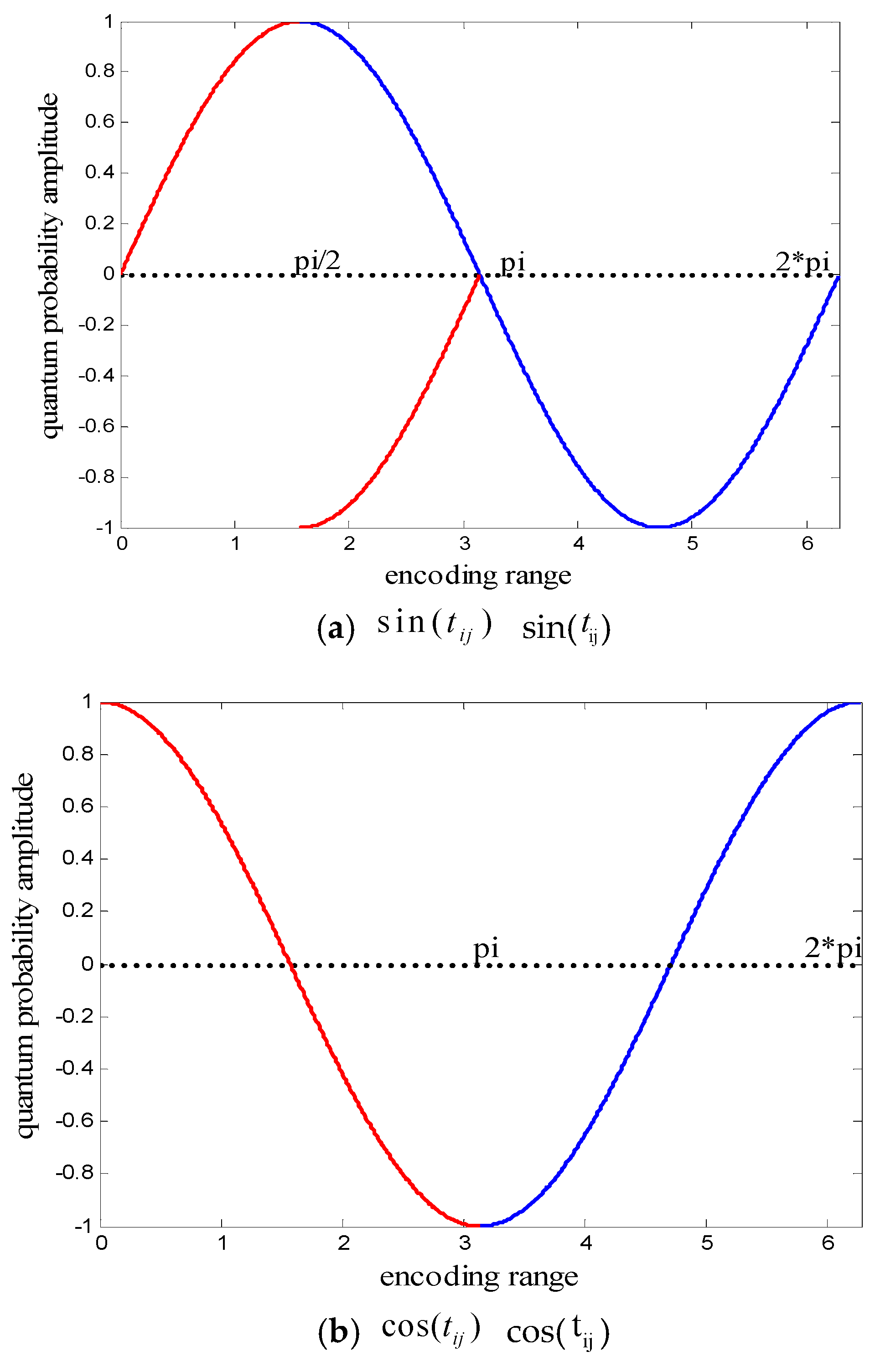
The coding space map of the two symmetry gene chains is shown in Figure 3. This improvement ensures that the probability amplitude of $\sin (t_{ij})$ and $\cos (t_{ij})$ are still within $(-1,1)$, and guarantees the monotonicity of the probability amplitude. Meanwhile, the new coding method increases the coding density (called high density coding) by reducing the search space, Thus enables the algorithm to get the optimal value faster.

Quantum Gate Updating: All evolutionary algorithms need to be updated in a specific way to improve population quality. In DCQGA, quantum rotation gates are defined as follows

$$U(\Delta \theta )=\left[\begin{array}{cc}\cos \Delta \theta & -\sin \Delta \theta \\ \sin \Delta \theta & \cos \Delta \theta \end{array}\right]$$

(18)

where $\Delta \theta$ is the rotation angle. By multiplying the original probability amplitude with the rotation door, we get the update effect of the quantum gene as follows:

$$\left[\begin{array}{c}\cos (t_i+\Delta \theta )\\ \sin (t_i+\Delta \theta )\end{array}\right]=\left[\begin{array}{cc}\cos \Delta \theta & -\sin \Delta \theta \\ \sin \Delta \theta & \cos \Delta \theta \end{array}\right]\left[\begin{array}{c}\cos (t_i)\\ \sin (t_i)\end{array}\right]$$

(19)

Quantum rotation gate mainly completes the quantum renewal process by changing the magnitude of probability. Therefore, $\Delta \theta$ is particularly important, too large $\Delta \theta$ will miss the optimum, too small $\Delta \theta$ will lead to the updated fitness value into the local optimal solution [24].

In IDCQGA, we use an adaptive rotation formula through the gradient of fitness, as shown below:

$$\Delta \theta =-\mathrm{sgn}(\left|\begin{array}{cc}{\alpha }_0& {\alpha }_i\\ {\beta }_0& {\beta }_i\end{array}\right|)\times \Delta {\theta }_0\times \exp (-\frac{\left|F(X_i^j)\right|-F_j\min }{F_j\max -F_j\min })$$

(20)

where $[{\alpha }_0{\beta }_0]$ and $[{\alpha }_i{\beta }_i]$ are the current and to be updated probability amplitudes; $\Delta {\theta }_0$ is the initial value; $F(X_i^j)$ is the fitness function value of the $i$-th qubit for the $j$-th chromosome; $F_j\min$ and $F_j\max$ are the minimum and maximum fitness function values.

It can be seen that this adaptive updating method is more reasonable, because when the gradient of fitness function is larger, the $\Delta \theta$ value is smaller, that is to say, the updating step is reduced, which ensures that the algorithm can search the optimal value more accurately. When the fitness function gradient is small, the value of $\Delta \theta$ is larger, that is, increasing the step size and improving the search speed of the algorithm.

Quantum chromosome mutation: In order to further increase the diversity of population size, optimization algorithms usually add mutation steps after population updating to avoid falling into local optimum as much as possible. The traditional algorithm uses NOT-gate mutation, and the quantum NOT-gate is defined as follows:

$$\left[\begin{array}{cc}0& 1\\ 1& 0\end{array}\right]=\left[\begin{array}{cc}\cos (\frac{\pi }{2})& \sin (\frac{\pi }{2})\\ \sin (\frac{\pi }{2})& -\cos (\frac{\pi }{2})\end{array}\right]$$

(21)

However, from the Equation (21), we can see that the principle of NOT-gate mutation is realized by the exchange of probability amplitude $\sin (t_{ij})$ and $\cos (t_{ij})$. This exchange method does not increase the diversity of probability amplitude, that is, it has little effect on the diversity of population size.

Therefore, in IDCQGA, we change the angle of the NOT-gate door and define $\pi /6$ mutation gate as follows:

$$U_{\frac{\pi }{6}}=\frac{1}{2}\left[\begin{array}{cc}\sqrt{3}& -1\\ 1& \sqrt{3}\end{array}\right]$$

(22)

The effect of $\pi /6$ mutation gate is:

$$\frac{1}{2}\left[\begin{array}{cc}\sqrt{3}& -1\\ 1& \sqrt{3}\end{array}\right]\left[\begin{array}{c}\cos (t_i)\\ \sin (t_i)\end{array}\right]=\left[\begin{array}{cc}\cos \frac{\pi }{6}& -\sin \frac{\pi }{6}\\ \sin \frac{\pi }{6}& \cos \frac{\pi }{6}\end{array}\right]\left[\begin{array}{c}\cos (t_i)\\ \sin (t_i)\end{array}\right]=\left[\begin{array}{c}\cos (\frac{\pi }{6}+t_i)\\ \sin (\frac{\pi }{6}+t_i)\end{array}\right]$$

(23)

It can be seen that the $\pi /6$ mutation gate changes the value of probability amplitude, which is a true sense of variation, thus enriching the size of the population. The value of $\pi /6$ can play a mutating role and avoid falling into local optimum as far as possible. In addition, the size of the value can be set according to the different experiments.

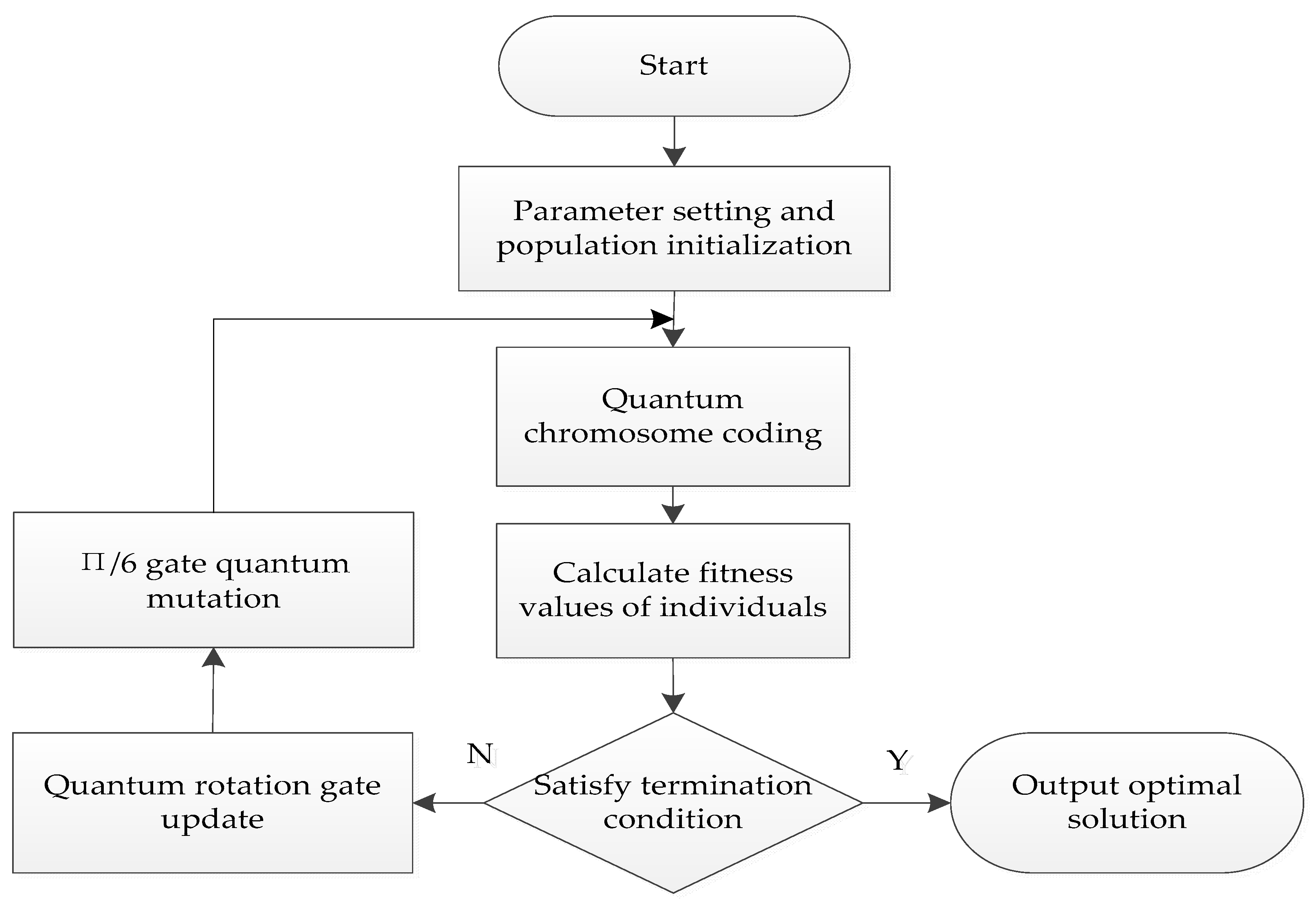
In order to apply the IDCQGA to the matching process of the optimal classification atoms, the signal separation degree D by the distance criterion should be used as the fitness function of the IDCQGA. The iterative process is shown in Figure 4.

3.3. Radar Signal Recognition

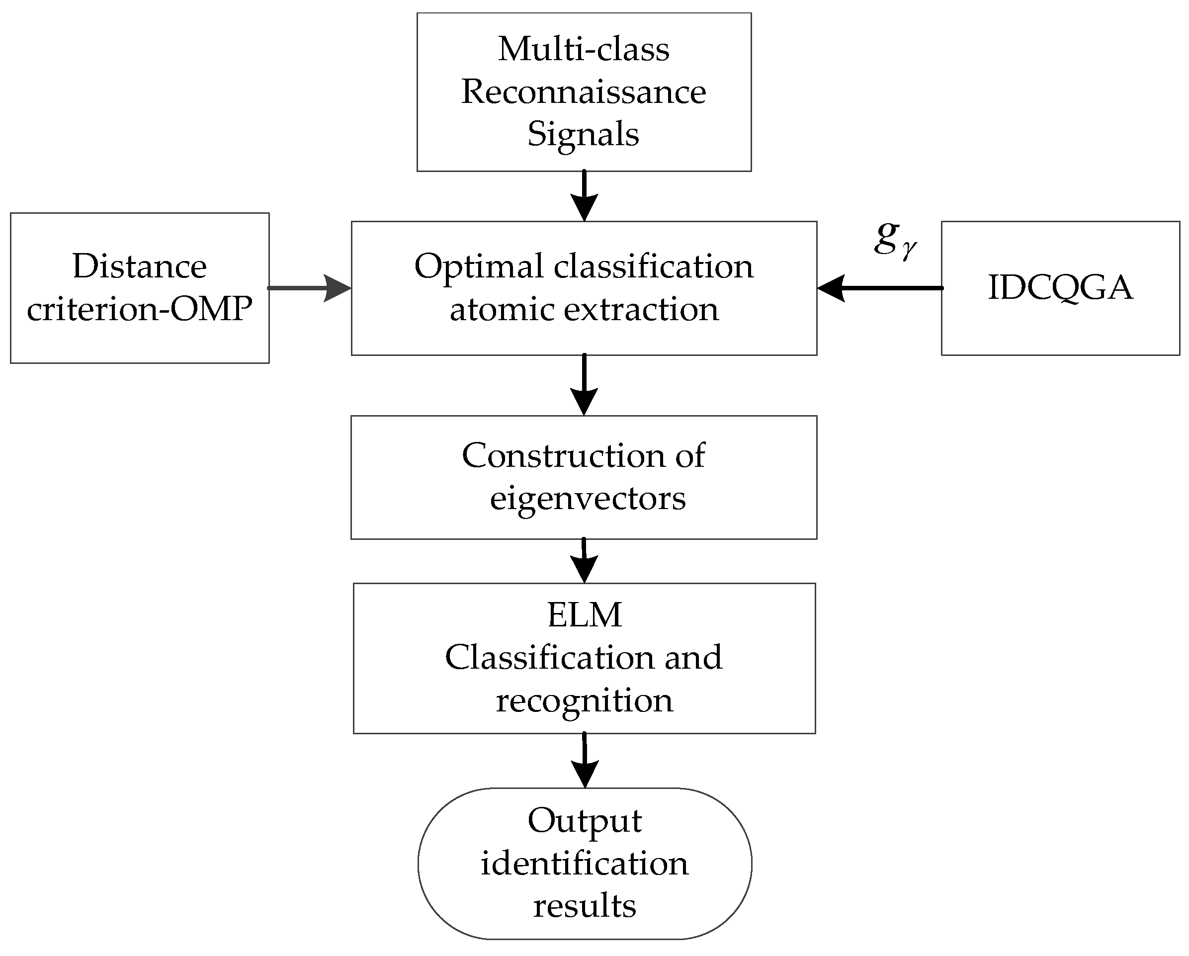
The proposed system structure of radar signal recognition is shown in Figure 5. IDCQGA can extract the optimal classification atoms of multi-class signals under the constraint of distance criterion-OMP, and then the optimal classification atoms and signals are internally product to get the eigenvectors. After the eigenvectors are determined, the classifier needs to recognize the feature vectors. SVM is suitable for small sample signal classification, but SVM needs to adopt additional intelligent algorithm to search for settings parameters. Therefore, this paper introduces the ELM algorithm with faster speed and less parameter settings to realize signal recognition. In ELM, activation function g(x) selects Sigmoidal function and the number of hidden layer nodes L can be obtained by grid search. Since the introduction of ELM is mainly to verify the effectiveness of the proposed feature extraction algorithm, this paper does not do much discussion on ELM, readers can refer to [29,30] for a detailed analysis of ELM.

The specific process is shown in Algorithm 1.

Algorithm 1 The specific process of signal recognition method.

Input: training and testing signals $C=\{f^{(i,j)},i=1,2,\dots c,j=1,2,\dots N_i\}$

Step1: Initialize population size, quantum gene number, maximum iteration number and mutation probability of IDCQGA. Initialize the iteration times of the distance criterion-OMP algorithm. Take atom $g_{\gamma }$ defined by the TF parameter $\gamma (s,u,\xi ,c)$ as the optimization parameters, signal separation degree $\left|D(f^{(i,j)},g_{\gamma })\right|$ is the fitness function. Step2: Search the maximum of fitness function and record the n optimal solutions $g_{\gamma }$. The n optimal solutions $g_{\gamma }$ represent the extracted optimal classification atoms. Step3: Obtain n-dimensional eigenvectors by inner multiplying n optimal classification atoms with all kinds of signals respectively. Then, normalize feature vectors to [0, 1]. Step4: Set randomly the weights w and offset b between the input and the hidden layer in ELM, and determine the number of hidden layer nodes L by grid search. Step5: Calculate the output matrix $H$ and the output weight $\beta$ of the network using the training set, and obtain the ELM model. Step6: Use ELM model to test the signal samples and evaluate the performance of the model.

Output: identification result of testing signals.

4. Simulation Results and Analysis

The following experiments are performed in MATLAB 2018(a) using Intel(R) Core i7-6700 + 4.0-GHz processor with the Windows 7 operating system. The proposed algorithm is in the analytical stage in a simulated computational environment.

4.1. Performance of IDCQGA

This section first uses the test function Shaffer’s F6 of the optimization algorithm to verify. The three-dimensional surface of the Shaffer’s F6 function as shown in Figure 6a–c are the profiles of $y=0$ and $x=0$. From Figure 6, we know that Shaffer’s F6 function has infinite maxima in (−100, 100), the maximum coordinate is (0, 0), the value is 1, the function expression is as follows:

$$S(x,y)=0.5-\frac{{\sin }^2\sqrt{x^2+y^2}-0.5}{{(1+0.001(x^2+y^2))}^2}\{\begin{array}{c}-100\le x\le 100\\ -100\le y\le 100\end{array}$$

(24)

Comparing the optimization performance of genetic algorithm (GA) [21], QGA [22], traditional DCQGA [24] and IDCQGA in this paper,

Table 1. Paramater setting of four optimazition algorithms.

Algorithm	Population Size	Bits of Gene	Encoding Method	Crossover Probability	Mutation Probability	Initial Rotation Angle	Evolutionary Generation
GA	50	100	Binary	0.7	0.05	-	120
QGA	10	100	qubit	-	-	-	120
DCQGA	10	2	Double-qubit	-	0.05	$0.01\pi$	120
IDCQGA	10	2	High-density	-	0.05	-	120

shows the parameter settings of each optimization algorithm.

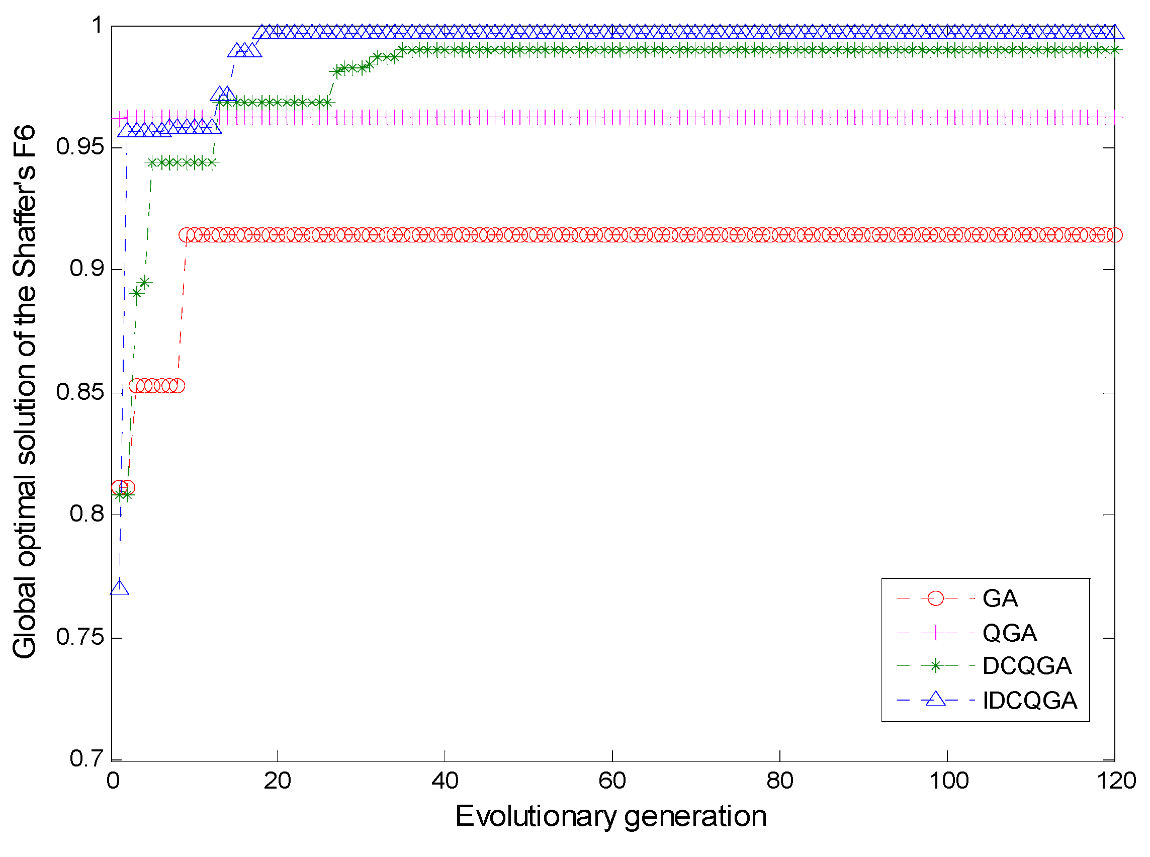
The optimization results of the four algorithms are shown in

Table 2. Simulation results of the optimization algorithm.

Algorithm	x	y	Best Result	Convergence Times
GA	18.0283	4.81177	0.77128	9
QGA	2.8985	5.5678	0.96278	1
DCQGA	−2.6202	−1.7276	0.99028	41
IDCQGA	1.52255	1.38334	0.99762	24

and Figure 7. The simulation results show that both GA and QGA are trapped in the local optimal value, only the optimal value of DCQGA and IDCQGA algorithm is greater than 0.99. QGA is the first to fall into local optimum, mainly because the fixed update steering angle limits the performance of the algorithm. The convergence algebra of IDCQGA is significantly lower than that of DCQGA, which shows that the high-density coding method in this paper compresses the search space of the algorithm and improves the convergence speed of the algorithm. At the same time, IDCQGA has the optimal maximum search value, and also verifies the feasibility of $\pi /6$ mutation gate.

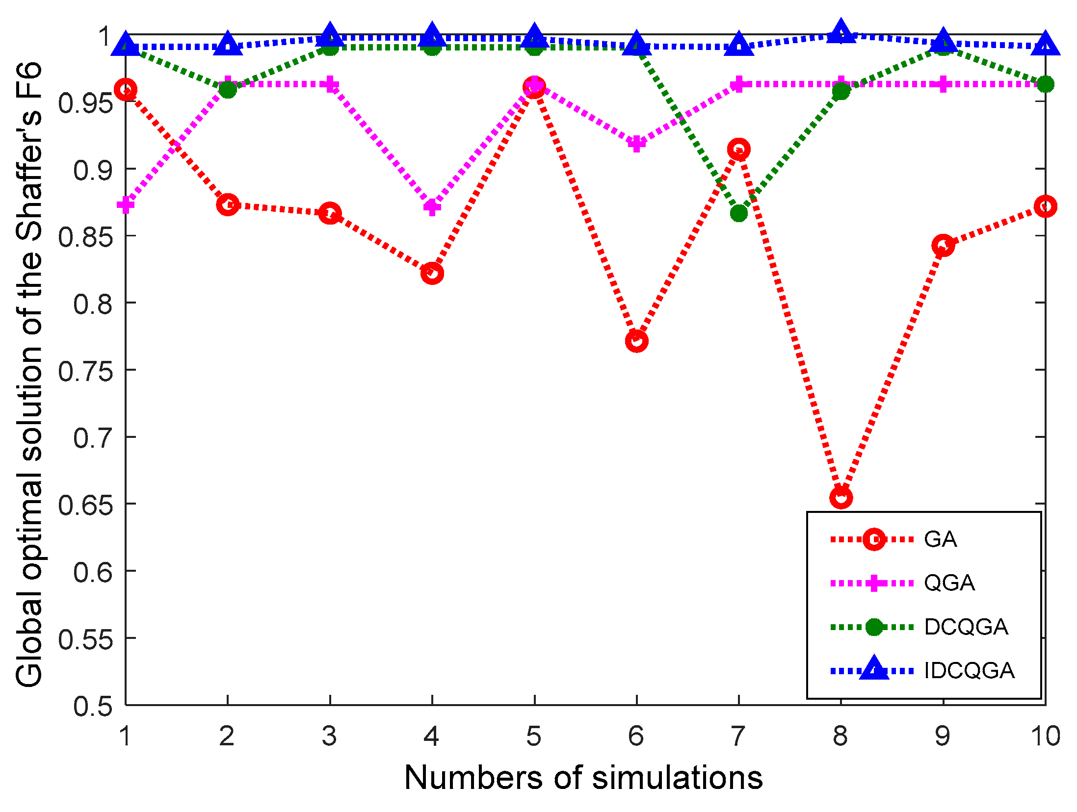
In order to further verify the stability of the four algorithms, each algorithm is tested 10 times, and the simulation results are shown in Figure 8. It can be seen that the biggest performance fluctuation of the algorithm is GA, followed by QGA. DCQGA algorithm achieves 6 times convergence state, and one optimization fluctuation is large. IDCQGA algorithm converges in 10 experiments, further verifying the stability of the proposed algorithm. For the optimization of complex functions, the high-density coding and mutation of the algorithm can improve the robustness and search performance of the algorithm, which is an excellent optimization algorithm. In the process of extracting the optimal classification atoms from the TF atom library, the fitness function of the optimization algorithm is replaced by the absolute value of the signal separation degree function.

4.2. Performance of the Optimal Classification Atoms

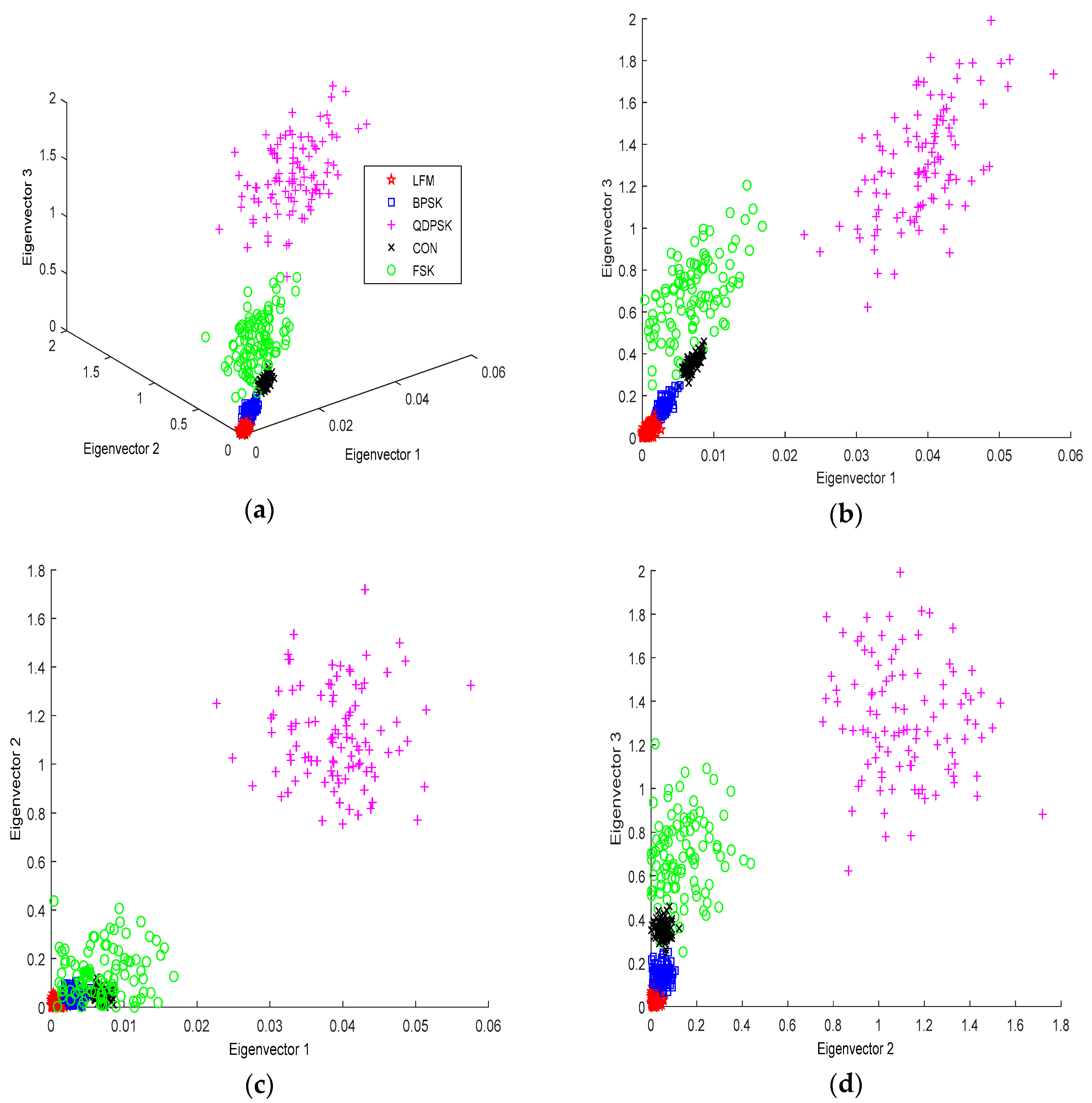
Firstly, five typical radar signals of linear frequency modulated (LFM), BPSK, quadrature phase-shift keying (QPSK), CON and binary frequency-shift keying (BFSK) are selected for verification. The pulse width of all signals is 10 us, sampling frequency is 100 MHz. For LFM, initial frequency is 5 MHz, bandwidth is 25 MHz; For BPSK and QPSK, the carrier frequency are 25 MHz, with 5-bir Barker coding and 16-bit Frank coding, respectively. For CON, the carrier frequency is 25 MHz; For BFSK, the lowest frequency is 10 MHz, the highest frequency is 25 MHz, with 7-bit Barker coding.

When the signal-noise-ratio (SNR) is 0 dB, 100 training samples and 100 test samples are randomly generated for each type of signal. Firstly, for the training sample set, 20 optimal classification atoms are selected by using the distance criterion-OMP (the number of atoms selected is obtained by many experiments) in Section 3.1. The parameters of the IDCQGA are as same as the experiment 4.1. The 20 optimal classification atoms are internally product with each training sample, and the 20-dimensional eigenvectors are obtained. In order to visualize the eigenvectors, the scatter plots and two-dimensional projection plots are drawn by selecting the first three-dimensional eigenvectors, as shown in Figure 9.

It can be seen that the first three-dimensional eigenvectors extracted from the five types of signals have good separation characteristics, especially the LFM, BPSK, CON have good intra-class aggregation. The intra-class aggregation of QPSK is relatively poor, but the inter-class separation between classes is better.

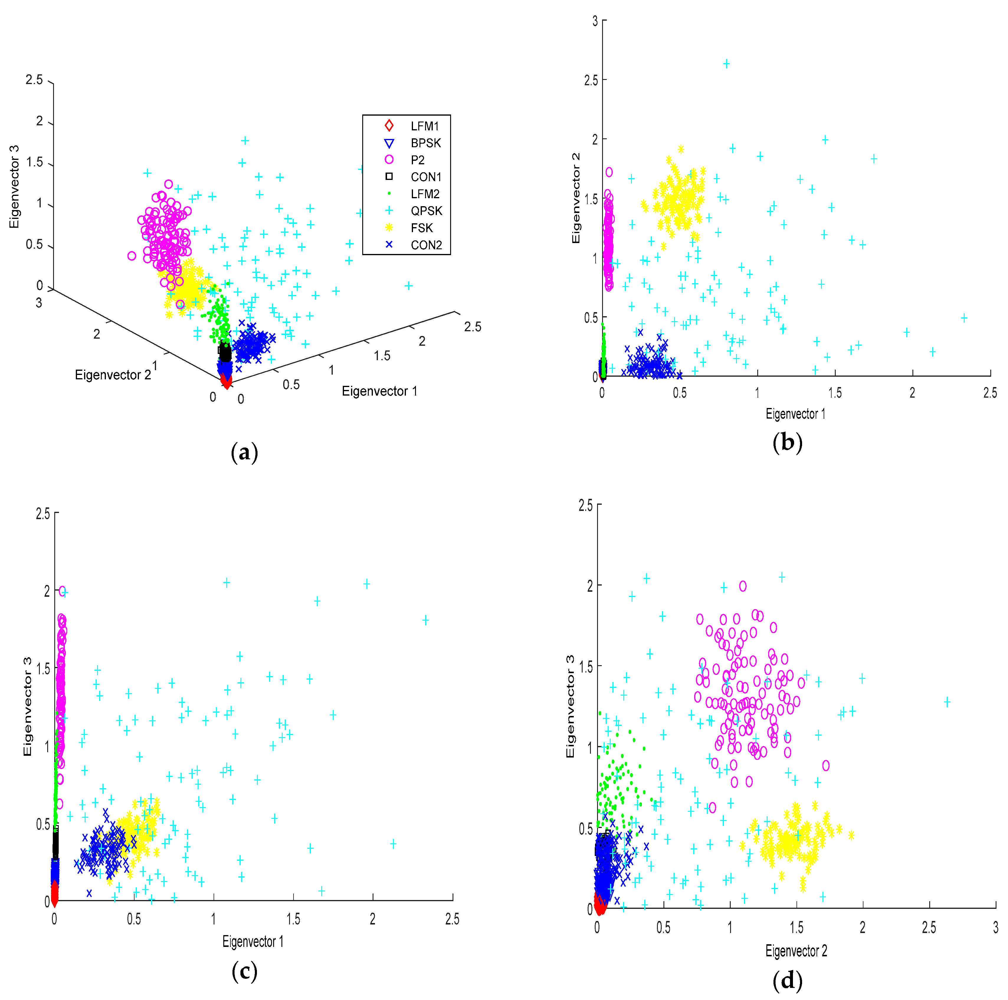
Then, the number of signal categories and the classification of similar signals are increased, LFM1, LFM2, BPSK, QPSK, CON1, CON2, BFSK, phase 2 (P2) eight types of radar signals are selected for simulation verification. For LFM1, initial frequency is 5 MHz, bandwidth is 10 MHz; For LFM2, initial frequency is 5 MHz, bandwidth is 20 MHz; For BPSK and QPSK, the parameters are same with the last experiment. For CON1 and CON2, the carrier frequency are 15 MHz and 10 MHz, respectively; For P2, the carrier frequency is 30 MHz, the sampling point of each step frequency is 4, the number of cycles of each phase code is 5; For BFSK; 13-bit Barker coding is used, the lowest frequency is 5 MHz, and the highest frequency is 15 MHz.

In the same way, a total of 800 training samples and 800 test samples are formed under the condition of 0 dB SNR. Firstly, for the training sample, 25 optimal classification atoms are selected by using the distance criterion-OMP in Section 3.1. The 25 optimal classifier atoms are internally product with each training sample, and 25-dimensional eigenvectors are obtained. The scatter plot and two-dimensional projection plot are also drawn by selecting the first three-dimensional eigenvectors, as shown in Figure 10.

It can be seen from Figure 9 and Figure 10 that the eigenvectors of the optimal classification atoms extracted by the proposed algorithm are separable to some extent. With the increase of the number of classes, the overlap of eigenvectors becomes more serious, especially for BPSK and QPSK signals. Under the condition of low SNR, the clustering of eigenvectors between classes is worse. This will bring difficulties to signal recognition. Under the condition of overlapping eigenvertors, the performance of recognition algorithm based on hard partition will be greatly affected. ELM can map the indivisible feature space to high-dimensional space to find the optimal partition. Therefore, it is reasonable to use ELM in this paper.

4.3. Performance of the Recognition Algorithm

Firstly, five typical radar signals in Experiment 4.2 are selected for simulation. In order to verify the performance of the algorithm under different SNR, each kind of signal is randomly generated 100 samples at −4–10 dB, respectively. The total number of training samples is 4000 (5 × 100 × 8 = 4000). Then, 4000 test samples were regenerated. In the ELM model, the parameter L range is [0, 1000], and L = 800 is obtained through grid search.

The experimental results under all SNR are shown in Figure 11. It can be seen from the graph that the recognition rate of the five kinds of signals basically increases with the increase of SNR. When SNR is −4 dB, the recognition rate of BPSK and QPSK less than 90%, which is consistent with the conclusion of experiment 4.2. When SNR is increased to 10 dB, the recognition rate of all signals is 100%. Thus, the detection signal recognition algorithm based on ELM is valid. In addition, the simulation results show that CON, LFM and FSK keep high recognition rate under the low SNR condition. This is mainly due to the high similarity between the three kinds of signals and the atoms in the Chirplet atom library. The extracted classification atoms can well express the main features of the signals. In the low SNR case, the TF atoms of BPSK and QPSK have a small discrimination, which results in a low signal recognition rate.

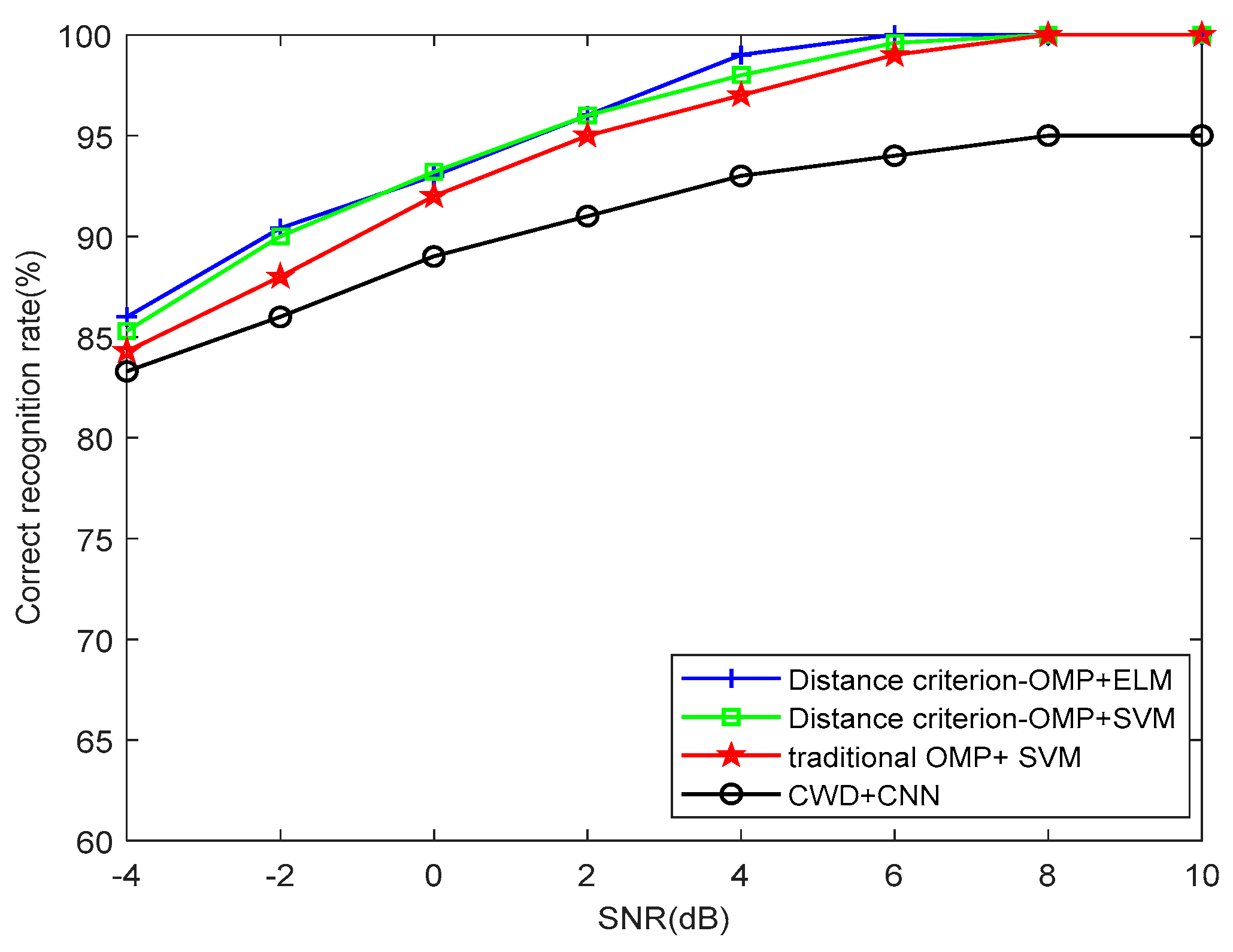
Then, eight kinds of radar signals in experiment 4.2 are selected. Each type of signal generated randomly 100 signal samples in −4–10 dB, a total of 6400 (8 × 100 × 8 = 6400) training samples. Then, 100 test samples of each class were regenerated in −4–10 dB, and 6400 samples were taken as test samples. The traditional OMP + SVM [9], recently proposed deep learning algorithm (CWD + CNN) [32], the proposed Distance criterion-OMP + SVM and Distance criterion-OMP + ELM are applied to compare and simulate, and the overall correct recognition rate is shown in Figure 12.

Figure 12 shows that the overall correct recognition rate of SVM and ELM algorithms is close, which verifies the feasibility and effectiveness of the proposed algorithm. Surprisingly, the effect of CWD + CNN is not ideal. In the case of low SNR, the anti-noise ability of the proposed algorithm is the best (0 dB, 92.6%). When the SNR rises to 8 dB, the recognition rate of the three algorithms for eight types of signals can reach more than 99%. The main reason is that the optimal classification atom can still better extract the atom features suitable for classification at low SNR. In the CWD + CNN algorithm [32], the signal is first converted into TF image. In order to make the size of TF image consistent, this algorithm first uses a series of image processing and clipping methods to get 32 × 32 pixel black-and-white image, and then sends it to the CNN classifier to get the recognition results. CWD + CNN algorithm works well for signals with frequency variation like LFM and Costas signals, but in this paper, the TF images of both CON1 and CON2 signals are a straight line, which makes the same 32 × 32 samples for the two types of signals after image clipping. Therefore, the recognition effect is not good for the single frequency component signals (such as CON1 and CON2). In this paper, the optimal classification atoms extracted by the proposed algorithm can clearly distinguish these signals with different carrier frequencies, which can avoid the confusion between the CON1 and CON2 signals.

Although the performance of ELM is similar to that of SVM, the complexity of ELM is lower than that of SVM (the CPU test time of SVM in this paper is three times as long as that of ELM). Meanwhile, the CWD + CNN algorithm is about 2 times the CPU test time of the proposed algorithm. The mainly reason is that in the CWD + CNN algorithm, the image preprocessing increases the complexity of the algorithm.

In order to analyze the proposed algorithm more accurately, which kind of signal has the lower recognition rate, the confusion matrixes of eight kinds of signal when extracting 0 dB are shown in

Table 3. The confusion matrix of eight types of signal at 0 dB by using CWD + CNN.

Signal Types	LFM1	LFM2	BPSK	QPSK	CON1	CON2	BFSK	P2
LFM1	88	2	1	0	5	4	0	0
LFM2	3	90	0	0	2	3	2	0
BPSK	0	0	91	6	0	3	0	0
QPSK	0	2	1	86	4	7	0	0
CON1	1	1	0	3	73	22	0	0
CON2	3	2	3	0	11	81	0	0
BFSK	0	0	0	0	0	0	100	0
P2	1	0	0	0	0	0	0	99

,

Table 4. The confusion matrix of eight types of signal at 0 dB by using tradition OMP + SVM.

Signal Types	LFM1	LFM2	BPSK	QPSK	CON1	CON2	BFSK	P2
LFM1	92	3	0	0	3	2	0	0
LFM2	2	95	0	0	1	1	1	0
BPSK	0	0	83	10	1	6	0	0
QPSK	0	2	9	81	3	5	0	0
CON1	2	0	0	3	93	2	0	0
CON2	1	0	1	0	3	95	0	0
BFSK	0	0	3	0	1	2	94	0
P2	1	0	0	0	0	0	1	98

and

Table 5. The confusion matrix of eight types of signal at 0 dB by using Distance criterion-OMP + ELM.

Signal Types	LFM1	LFM2	BPSK	QPSK	CON1	CON2	BFSK	P2
LFM1	93	2	0	0	3	2	0	0
LFM2	2	95	0	0	1	1	1	0
BPSK	0	0	89	7	2	2	0	0
QPSK	0	2	6	85	4	3	0	0
CON1	1	0	0	3	94	2	0	0
CON2	1	0	1	0	1	96	1	0
BFSK	0	0	3	0	1	3	93	0
P2	2	1	0	0	0	0	1	96

.

Comparing Table 3 and Table 5, we can see that CWD + CNN algorithm is easy to confuse CON1 and CON2 signals, which also validates our previous discussion. Meanwhile, From Table 5, it can be seen that BPSK has 7 signals mistakenly identified as QPSK, and QPSK is mistaken for BPSK with 6 signals. Compared with Table 4, the confusing BPSK and QPSK signals have been reduced to some extent. Similar to the five types of signals, BPSK and QPSK still have lower recognition rate, mainly because the TF atoms of the same kind of signals (LFM2 and CON2) are similar to BPSK and QPSK, which further increases the difficulty of signal recognition. Experiments 4.2 and 4.3 show that the proposed optimal classification atom can be used as an element to construct eigenvectors, and it still has higher recognition than OMP algorithm in the low SNR case. At the same time, considering the fast convergence speed in the training process of ELM algorithm and the recognition effect similar to SVM algorithm, it is reasonable to select ELM as the classifier. Especially for the overlapping data, the ELM algorithm can map the indivisible feature space to the high-dimensional separable space to realize complex signal recognition.

5. Conclusions

In this paper, the waveform feature extraction and recognition method of radar electronic reconnaissance signal is mainly studied. Firstly, by analyzing the problems existing in traditional atom matching decomposition algorithm, an optimum classification atom feature extraction method is proposed, which establishes the signal separation degree between different signal waveforms using distance criterion. Then, TF atoms with larger signal separation degree are extracted to construct the classification atom set, and the inner product of signal and selected atom is applied as the eigenvectors. Finally, ELM is introduced as the classifier to complete the signal recognition, which effectively improves the recognition performance of signal in the presence of overlapping eigenvectors. Simulation results show that the proposed algorithm has better stability and anti-noise performance than the traditional OMP matching pursuit and SVM recognition algorithm. When the SNR is 0 dB, the signal recognition rate of the proposed algorithm reaches 92.6%, which provides a new scheme for the classification and recognition of radar signals in electronic reconnaissance.

It is important to note that we explore a wide radar signal recognition system to classify, but not identify, in this paper. In radar field, the meaning of “classify” is that distinguish the different types of signals, while “identify” means recognition particular copies of the same radar type. The latter is called Specific Emitter Identification (SEI). SEI is based on intra-pulse analysis, use of out-of-band radiation, use of fractal theory, and other methods by which it is possible to extract additional features from the radar signal [33,34,35,36]. Since SEI technology is also an important subject in the field of electronic reconnaissance, we intend to conduct in-depth analysis of this subject in the next step.