Triangular Cubic Hesitant Fuzzy Einstein Hybrid Weighted Averaging Operator and Its Application to Decision Making

Abstract

In this paper, triangular cubic hesitant fuzzy Einstein weighted averaging (TCHFEWA) operator, triangular cubic hesitant fuzzy Einstein ordered weighted averaging (TCHFEOWA) operator and triangular cubic hesitant fuzzy Einstein hybrid weighted averaging (TCHFEHWA) operator are proposed. An approach to multiple attribute group decision making with linguistic information is developed based on the TCHFEWA and the TCHFEHWA operators. Furthermore, we establish various properties of these operators and derive the relationship between the proposed operators and the existing aggregation operators. Finally, a numerical example is provided to demonstrate the application of the established approach.

1. Introduction

Multicriteria decision-making (MCDM) problems seek great attention to practical fields, whose target is to find the best alternative(s) among the feasible options. In primitive times, decisions were framed without handling the uncertainties in the data, which may lead to inadequate results toward the real-life operating situations. Since all these facilitate the uncertainties to a great extent, they cannot withstand situations where the decision the maker has to consider the falsity corresponding to the truth a value ranging over an interval. IFSs have the advantage that permits the user to model some uncertainty on the membership function of the elements. That is, fuzzy sets require a membership degree for each element in the reference set, whereas an IFS permits us to include some hesitation on this value. Atanassov [1] originated the notion of intuitionistic fuzzy set (IFS), which is a generalization of Zadeh’s fuzzy sets [2]. The intuitionistic fuzzy set has three main parts: membership function, non-membership function, and hesitancy function. According to Zadeh [3], a conditional statement “If $x=A$ then $y=$” describes a relation between the two fuzzy variables x and y. He therefore suggests that the conditional statement should be represented by a fuzzy relation from U and V. Bustince et al. [4] analysed the existent relations between the structures of a relation and the structures of its complementary one. Deschrijver et al. [5] introduced the many theories to establish the relationships between intuitionistic fuzzy sets, interval-valued fuzzy sets, and interval-valued intuitionistic fuzzy sets. Through the last period, the AIFS theory has been suitably associated with aggregate intuitionistic fuzzy information [6,7]. Xu [8] developed some basic arithmetic aggregation operators, such as the intuitionistic fuzzy weighted averaging (IFWA) operator, intuitionistic fuzzy ordered weighted averaging (IFOWA) operator, and intuitionistic fuzzy hybrid averaging (IFHA) operator, for aggregating intuitionistic fuzzy values (IFVs). Chen and Xu [9] presented a structure which generalizes the idea of HFS [10] to IVHFS that makes possible the membership evaluation of a component into many realizable interval numbers. Torra [10] proposed the hesitant fuzzy set that permitted the membership having a set of possible values and discussed the relationship between the hesitant fuzzy set and intuitionistic fuzzy set. The hesitant fuzzy set can be applied to many decision-making problems. He also proved that the operations he proposed are consistent with the ones of the intuitionistic fuzzy set when applied to the envelope of the hesitant fuzzy set. To get the optimal alternative in a decision making problem with multiple attributes and multiple persons, there are usually two ways: (1) aggregate the decision makers’ opinions under each attribute for alternatives, then aggregate the collective values of attributes for each alternative; (2) aggregate the attribute values given by the decision makers for each alternative, and then aggregate the decision makers’ opinions for each alternative. Xia et al. [11] developed some operations and aggregation operators for hesitant fuzzy elements. Xia et al. [12] defined the reflect the correlation of the aggregation arguments, two methods are proposed to determine the aggregation weight vectors. Zeng et al. [13] developed an intuitionistic fuzzy ordered weighted distance (IFOWD) operator.

Decision-making is an integral part of modern management. Essentially, rational or sound decision making is taken as a primary function of management. Every manager takes hundreds and hundreds of decisions subconsciously or consciously making it as the key component in the role of a manager. Decisions play important roles as they determine both organizational and managerial activities. A decision can be defined as a course of action purposely chosen from a set of alternatives to achieve organizational or managerial objectives or goals. A decision-making process is a continuous and indispensable component of managing any organization or business activities. Decisions are made to sustain the activities of all business activities and organizational functioning. Decision theory has its root in economic theory, with the assumption that people make decisions to maximize utility on the basis of self-interest and rationality. This, however, does not consider the possibilities or effects of moderating or intervening factors that make decisions reference-dependent. Nonetheless, expected utility theory has been applied in the construction industry with some success and has been the predominant model for normative decision making. The theory is considered idealistic, however, because it focuses on how managers should make decisions rather than how they actually make decisions.

Technical people in the construction industry have been observed to exhibit a tendency for a normative approach to decision making, thereby weakening their ability to deal with uncertainty. Program management is dominated by technical staff and probably more than a few are struggling with tendencies toward this normative thinking phenomenon. An alternative approach is the descriptive decision theory.

Comparative analysis needs to be distinguished from the juxtaposition of descriptions of a series of cases. While sequential presentations of descriptive data are undoubtedly informative about the cases concerned they are only comparative in the weak sense of making the reader aware of differences and similarities. They whet the appetite to know more. Based on the algebraic sum, algebraic product, and operational laws on AIFSs, some aggregation operators have been proposed to overcome the lack of precision in the final results using the binary operations to carry the combination process. Xu and Yager [14] developed some basic geometric aggregation operators such as intuitionistic fuzzy weighted geometric (IFWG) operator, intuitionistic fuzzy ordered weighted geometric (IFOWG) operator, and intuitionistic fuzzy hybrid geometric (IFHG) operator, and applied them to multiple attribute decision making (MADM) based on AIFSs. Xu and Yager [15] defined dynamic IFWA operator and developed a procedure to solve the dynamic intuitionistic fuzzy MADM problems. Zhao et al. [16] developed some hesitant triangular fuzzy aggregation operators based on the Einstein operation: the hesitant triangular fuzzy Einstein weighted averaging (HTFEWA) operator, hesitant triangular fuzzy Einstein weighted geometric (HTFEWG) operator, hesitant triangular fuzzy Einstein ordered weighted averaging (HTFEOWA) operator, hesitant triangular fuzzy Einstein ordered weighted geometric (HTFEOWG) operator, hesitant triangular fuzzy Einstein hybrid average (HTFEHA) operator and hesitant triangular fuzzy Einstein hybrid geometric (HTFEHG) operator. Li et al. [17] developed to introduce some concepts of fuzzy measure and interval-valued intuitionistic uncertain linguistic variables based on Archimedean t-norm. Then, interval-valued intuitionistic uncertain linguistic weighted average(geometric) and interval-valued intuitionistic uncertain linguistic ordered weighted average operator based on Archimedean t-norm are developed. Furthermore, some desirable properties of these operators, such as commutativity, idempotency, and monotonicity have been studied, and interval-valued intuitionistic uncertain linguistic hybrid average operator based on Archimedean t-norm are developed.

Cubic set was introduced by Jun et al. [18]. Cubic sets are the extensions of fuzzy sets and intuitionistic fuzzy sets, in which there are two representations, one is utilized for the degree of membership and other is utilized for the degree of non-membership. The membership function is grip as interval while non-membership is thoroughly considered the ordinary fuzzy set.

Medina et al. [19] showed that the information common to both concept lattices can be seen as a sublattice of the Cartesian product of both concept lattices. Pozna et al. [20] proposed the attractive applications of signatures related to the modeling of fuzzy inference systems suggested and discussed. Jankowski et al. [21] proposed model revealed that a growing level of persuasion can increase results only to a certain extent. Kumar et al. [22] proposed the Artificial Bee Colony (ABC) algorithm is a swarm-based algorithm inspired by the intelligent foraging behavior of honey bees. In order to make use of the merits of both algorithms, a hybrid algorithm (IABCFCM) based on improved ABC and FCM algorithms.

Chen et al. [23] developed some hesitant triangular intuitionistic fuzzy aggregation operators and standardized hesitant triangular intuitionistic fuzzy aggregation operators. Xu et al. [24] provided a survey of the aggregation techniques of intuitionistic fuzzy information, and their applications in various fields, such as decision making, cluster analysis, medical diagnosis, forecasting, and manufacturing grid. Zhang [25] developed a series of aggregation operators for interval-valued intuitionistic hesitant fuzzy information.

Fahmi et al. [26] developed the hamming distance for the triangular cubic fuzzy number and weighted averaging operator. Fahmi et al. [27] proposed the cubic TOPSIS method and grey relational analysis set. Fahmi et al. [28] defined the triangular cubic fuzzy number and operational laws. The authors developed the triangular cubic fuzzy hybrid aggregation (TCFHA) administrator to total all individual fuzzy choice structure provided by the decision makers into the aggregate cubic fuzzy decision matrix. Amin et al. [29] defined the generalized triangular cubic linguistic hesitant fuzzy weighted geometric (GTCHFWG) operator, generalized triangular cubic linguistic hesitant fuzzy ordered weighted average (GTCLHFOWA) operator, generalized triangular cubic linguistic hesitant fuzzy ordered weighted geometric (GTCLHFOWG) operator, generalized triangular cubic linguistic hesitant fuzzy hybrid averaging (GTCLHFHA) operator and generalized triangular cubic linguistic hesitant fuzzy hybrid geometric (GTCLHFHG) operator. Fahmi et al. [30] developed Trapezoidal linguistic cubic hesitant fuzzy TOPSIS method to solve the MCDM method based on trapezoidal linguistic cubic hesitant fuzzy TOPSIS method. Fahmi et al. [31] define aggregation operators for triangular cubic linguistic hesitant fuzzy sets which include cubic linguistic fuzzy (geometric) operator, triangular cubic linguistic hesitant fuzzy weighted geometric (TCLHFWG) operator, triangular cubic linguistic hesitant fuzzy ordered weighted geometric (TCHFOWG) operator and triangular cubic linguistic hesitant fuzzy hybrid geometric (TCLHFHG) operator. Fahmi et al. [32] defined the trapezoidal cubic fuzzy weighted arithmetic averaging operator and weighted geometric averaging operator. Expected values, score function, and accuracy function of trapezoidal cubic fuzzy numbers are defined. Fahmi et al. [33] developed three arithmetic averaging operators, that is trapezoidal cubic fuzzy Einstein weighted averaging (TrCFEWA) operator, trapezoidal cubic fuzzy Einstein ordered weighted averaging (TrCFEOWA) operator and trapezoidal cubic fuzzy Einstein hybrid weighted averaging (TrCFEHWA) operator, for aggregating trapezoidal cubic fuzzy information. Fahmi et al. [34] defined some Einstein operations on cubic fuzzy set (CFS) and develop three arithmetic averaging operators, which are cubic fuzzy Einstein weighted averaging (CFEWA) operator, cubic fuzzy Einstein ordered weighted averaging (CFEOWA) operator and cubic fuzzy Einstein hybrid weighted averaging (CFEHWA) operator, for aggregating cubic fuzzy data. Amin et al. [35] introduced the new concept of the trapezoidal cubic hesitant fuzzy TOPSIS method.

Despite having a bulk of related literature on the problem under consideration, the following aspects related to triangular cubic hesitant fuzzy numbers (TCHFNs) and their aggregation operators motivated the researchers to carry it an in depth inquiry into the current study.

(1) The main advantages of the proposed operators are these aggregation operators provided more accurate and precious result as compare to the above mention operators.

(2) We generalized the concept of triangular cubic hesitant fuzzy numbers (TCHFNs), triangular intuitionistic fuzzy sets and introduce the concept of triangular cubic hesitant fuzzy numbers. If we take only one element in the membership degree of the triangular cubic hesitant fuzzy number, i.e., instead of the interval we take a fuzzy number, then we get triangular intuitionistic fuzzy numbers, similarly, if we take membership degree as the fuzzy number and non-membership degree equal to zero, then we get triangular fuzzy numbers.

(3) The objective of the study include:

Propose triangular cubic hesitant fuzzy number, operational laws, score value and accuracy value of TCHFNs.

Propose three aggregation operators, namely Triangular cubic hesitant fuzzy Einstein weighted averaging operator, Triangular cubic hesitant fuzzy Einstein ordered weighted averaging operator and Triangular cubic hesitant fuzzy Einstein hybrid weighted averaging operator.

Establish MADM program approach based triangular cubic hesitant fuzzy numbers.

Provide illustrative examples of MADM program.

(4) In order to testify the application of the developed method, we apply the triangular cubic hesitant fuzzy numbers in the decision making.

(5)The initial decision matrix is composed of LVs. In order to fully consider the randomness and ambiguity of the linguistic term, we convert LVs into the triangular cubic hesitant fuzzy numbers, and the decision matrix is transformed into the triangular cubic hesitant fuzzy matrix.

(6)The operator can fully express the uncertainty of the qualitative concept and triangular cubic hesitant fuzzy operators can capture the interdependencies among any multiple inputs or attributes by a variable parameter. The aggregation operators can take into account the importance of the attribute weights. Nevertheless, sometimes, for some MAGDM problems, the weights of the attributes are important factors for the decision process.

(7) As we have discussed earlier that Cubic sets are the generalization of intuitionistic hesitant fuzzy sets and a powerful tool to deal with fuzziness. Also, triangular intuitionistic hesitant fuzzy numbers are suitable to deal with fuzziness. However, there may be a situation where the decision maker may provide the degree of membership and nonmembership of a particular attribute in such a way that membership degree is a triangular interval hesitant fuzzy number and non-membership degree is a triangular hesitant fuzzy number. Therefore, to overcome this shortcoming we generalize the concept of triangular intuitionistic hesitant fuzzy numbers and introduce the concept of triangular cubic hesitant fuzzy sets which are very suitable to be used for depicting uncertain or hesitant fuzzy information. If we take only one element in the membership degree of the triangular cubic hesitant fuzzy number, i.e., instead of interval we take a hesitant fuzzy number, then we get triangular intuitionistic hesitant fuzzy numbers, similarly if we take membership degree as hesitant fuzzy number and nonmemberíship degree equal to zero, than we get triangular hesitant fuzzy numbers. Thus motivating by the idea proposed by Zhao et al. [16], in this paper we first proposed triangular cubic hesitant fuzzy number and including the Triangular cubic hesitant fuzzy Einstein weighted averaging (TCHFEWA) operator, triangular cubic hesitant fuzzy einstein ordered weighted averaging (TCHFEOWA) operator and triangular cubic hesitant fuzzy einstein hybrid weighted averaging (TCHFEHWA) operator.

This paper is organized as follows. In Section 2, we discuss some basic ideas to the fuzzy set and cubic set. In Section 3, we define the triangular cubic hesitant fuzzy numbers (TCHFNs) and operational laws. In Section 4, we present some Einstein operations on triangular cubic hesitant fuzzy numbers (TCHFNs) and analysis some desirable properties of the suggested operations. In Section 5, we first develop some novel arithmetic averaging operators, such as the triangular cubic hesitant fuzzy Einstein weighted averaging (TCHFEWA) operator, triangular cubic hesitant fuzzy Einstein ordered weighted averaging (TCHFEOWA) operator and triangular cubic hesitant fuzzy Einstein hybrid weighted averaging (TCHFEHWA) operator, for aggregating a collection of triangular cubic hesitant fuzzy numbers (TCHFNs). In Section 6, we relate the TCHFEHWA operator to MADM with triangular cubic hesitant fuzzy material. In Section 7, gives an example to illustrate the application of the developed method. In Section 8, we propose the comparison method. In Section 9, we consume a conclusion.

2. Preliminaries

Definition 1.

[2] Let H be a universe of discourse. Then the fuzzy set can be defined as: $J=\{\ddot{h},{\Gamma }_J(\ddot{h})|\ddot{h}\in H\}.$ A fuzzy set in a set H is denoted by ${\Gamma }_J:H\to I.$ The function ${\Gamma }_J(\ddot{h})$ denoted the degree of membership of the element $\ddot{h}$ to the set H, where $I=[0,1]$. The gathering of all fuzzy subsets of H is denoted by $I^H$. Define a relation on $I^H$ as follows: $(\forall \Gamma ,\eta \in I^H)(\Gamma \le \eta \iff (\forall \ddot{h}\in \ddot{h})(\Gamma (\ddot{h})\le \eta (\ddot{h}))).$

Definition 2.

[1] Let a set H be fixed, an AIFS A in H is defined as:

$A=\left\{\langle \ddot{h},{\Gamma }_A(\ddot{h}),{\eta }_A(\ddot{h})\rangle |\ddot{h}\in H\right\}$ where ${\Gamma }_A$ and ${\eta }_A$ are mapping from H to the closed interval $[0,1]$ such that $0\le {\Gamma }_A\le 1,0\le {\eta }_A\le 1$ and $0\le {\Gamma }_A(\ddot{h})+{\eta }_A(\ddot{h})\le 1,$ for all $\ddot{h}\in H,$ and they denote the degrees of membership and non-membership of element $\ddot{h}\in H$ to set $A,$ respectively. Let ${\pi }_A(\ddot{h})=1-{\Gamma }_A(\ddot{h})-{\eta }_A(\ddot{h}),$ then it is usually called the intuitionistic fuzzy index of element $\ddot{h}\in H$ to set A, representing the degree of indeterminacy or hesitation of $\ddot{h}$ to A. It is obvious that $0\le {\pi }_A(\ddot{h})\le 1$ for every $\ddot{h}\in H$.

Definition 3.

[18] Let H is a nonempty set. By a cubic set in H we mean a structure $F=\{h,\alpha (h),\ddot{\beta }(h):h\in H\}$ in which α is an IVF set in H and $\ddot{\beta }$ is a fuzzy set in $H.$ A cubic set $F=\{h,\alpha (h),\ddot{\beta }(h):h\in H\}$ is simply denoted by $F=\langle \alpha ,\ddot{\beta }\rangle .$ Denote by ${\ddot{c}}^H$ the collection of all cubic sets in $H.$ A cubic set $F=\langle \alpha ,\ddot{\beta }\rangle$ in which $\alpha (h)=0$ and $\ddot{\beta }(h)=1$(resp.$\alpha (h)=1$ And $\ddot{\beta }(h)=0$ for all $h\in H$ is denoted by 0 (resp. 1). A cubic set $\stackrel{⃛}{D}=\langle \lambda ,\xi \rangle$ in which $\lambda (h)=0$ and $\xi (h)=0$ (resp.$\lambda (h)=1$ and $\xi (h)=1$) for all $h\in H$ is denoted by 0 (resp. 1).

Definition 4.

[18] Let H is a non-empty set. A cubic set $F=(\ddot{c},\lambda )$ in H is said to be an internal cubic set if ${\ddot{c}}^{-}(h)\le \lambda (h)\le {\ddot{c}}^{+}(h)$$\forall h\in H.$

Definition 5.

[18] Let H is a non-empty set. A cubic set $F=(\ddot{c},\lambda )$ in H is said to be an external cubic set if $\lambda (h)\notin ({\ddot{c}}^{-}(h),{\ddot{c}}^{+}(h))$$\forall h\in H.$

Definition 6.

[36] Triangular fuzzy number is defined as $A=\{a,b,c\},$ where $a,b,c$ are real number and its membership function is given below

$${\mu }_A(x)=\left\{\begin{array}{cc}0& \mathit{for}x<a\\ \left\{\frac{(x-a)}{(b-a)}\right\}& a\le x\le b\\ 1& \mathit{for}x=b\\ \left\{\frac{(c-x)}{(c-b)}\right\}& b<x\le c\\ 0& \mathit{for}x>c\end{array}\right.$$

Definition 7.

[36] Let X be a fixed set, a triangular hesitant fuzzy set defined by $A=\{<x,T{h}_A(x)>\backslash x\in X\},$ where $T{h}_A(x)$ is a set of some triangular values in $\left(a^L,a^M,a^U\right).$

3. Triangular Cubic Hesitant Fuzzy Number and Operational Laws

Definition 8.

Let $\tilde{b}$ be the triangular cubic hesitant fuzzy number on the set of real numbers, its interval-valued triangular hesitant fuzzy set is defined as follows:

$${\lambda }_{\tilde{b}}(h)=\left\{\begin{array}{cc}\{\frac{(h-p^{-})}{(q^{-}-p^{-})},\frac{(h-p^{+})}{(q^{+}-p^{+})}\}& (p^{-},q^{-})\le h<(p^{+},q^{+})\\ \{\frac{(r^{-}-h)}{(r^{-}-q^{-})},\frac{(r^{+}-h)}{(r^{+}-q^{+})}\}& (q^{-},r^{-})\le h<(q^{+},r^{+})\\ 0& otherwise\end{array}\right.$$

and its triangular hesitant fuzzy set is

${\Gamma }_{\tilde{b}}(h)=\left\{\begin{array}{cc}\left\{\frac{(q-h)}{(q-p)}\right\}& p\le h<q\\ \left\{\frac{(r-h)}{(r-q)}\right\}& q<h\le r\\ 0& otherwise\end{array}\right.$ where $0\le {\lambda }_{\tilde{b}}(h)\le 1,0\le {\Gamma }_{\tilde{b}}(h)\le 1$. Then the TCHFN $\tilde{b}$ is given by $\tilde{b}$ $=〈\begin{array}{c}[p^{-},q^{-},r^{-}],\\ p^{+},q^{+},r^{+}],\\ [p,q,r]\end{array}〉$ and $\tilde{b}$ is called triangular cubic hesitant fuzzy number.

Definition 9.

Let ${\ddot{A}}_1=\left\{\begin{array}{c}\langle [p_1^{-}(\stackrel{⃛}{z}),\\ q_1^{-}(\stackrel{⃛}{z}),r_1^{-}(\stackrel{⃛}{z})],\\ [p_1^{+}(\stackrel{⃛}{z}),\\ q_1^{+}(\stackrel{⃛}{z}),r_1^{+}(\stackrel{⃛}{z})],\\ [p_1(\stackrel{⃛}{z}),\\ q_1(\stackrel{⃛}{z}),r_1(\stackrel{⃛}{z})]\rangle \\ |\stackrel{⃛}{z}\in Z\end{array}\right\}$ and ${\ddot{A}}_2=\left\{\begin{array}{c}\langle [p_2^{-}(\stackrel{⃛}{z}),\\ q_2^{-}(\stackrel{⃛}{z}),r_2^{-}(\stackrel{⃛}{z})],\\ [p_2^{+}(\stackrel{⃛}{z}),\\ q_2^{+}(\stackrel{⃛}{z}),r_2^{+}(\stackrel{⃛}{z})],\\ [p_2(\stackrel{⃛}{z}),\\ q_2(\stackrel{⃛}{z}),r_2(\stackrel{⃛}{z})]\rangle \\ |\stackrel{⃛}{z}\in Z\end{array}\right\}$ are two triangular cubic hesitant fuzzy numbers (TCHFNs), some operations on triangular cubic hesitant fuzzy numbers (TCHFSs) are defined as follows:

$$\left\{\begin{array}{c}{\ddot{A}}_1\subseteq {\ddot{A}}_{2}iff\forall \stackrel{⃛}{z}\in Z,p_1^{-}(\stackrel{⃛}{z})\ge p_2^{-}(\stackrel{⃛}{z}),q_1^{-}(\stackrel{⃛}{z})\ge q_2^{-}(\stackrel{⃛}{z}),\\ r_1^{-}(\stackrel{⃛}{z})\ge r_1^{-}(\stackrel{⃛}{z}),p_1^{+}(\stackrel{⃛}{z})\ge p_2^{+}(\stackrel{⃛}{z}),q_1^{+}(\stackrel{⃛}{z})\ge q_2^{+}(\stackrel{⃛}{z}),\\ r_1^{+}(\stackrel{⃛}{z})\ge r_1^{+}(\stackrel{⃛}{z})\mathrm{and}{p}_1(\stackrel{⃛}{z})\le p_2(\stackrel{⃛}{z}),q_1(\stackrel{⃛}{z})\le q_2(\stackrel{⃛}{z}),\\ r_1(\stackrel{⃛}{z})\le r_2(\stackrel{⃛}{z})\end{array}\right\}$$

(1)

$${\ddot{A}}_1{\cap }_{T,S}{\ddot{A}}_2=〈\begin{array}{c}T[p_1^{-}(\stackrel{⃛}{z}),p_2^{-}(\stackrel{⃛}{z})],T[q_1^{-}(\stackrel{⃛}{z}),q_2^{-}(\stackrel{⃛}{z})],\\ T[r_1^{-}(\stackrel{⃛}{z}),r_2^{-}(\stackrel{⃛}{z})],T[p_1^{+}(\stackrel{⃛}{z}),p_2^{+}(\stackrel{⃛}{z})],\\ T[q_1^{+}(\stackrel{⃛}{z}),q_2^{+}(\stackrel{⃛}{z})],T[r_1^{+}(\stackrel{⃛}{z}),r_2^{+}(\stackrel{⃛}{z})],\\ S[p_1(\stackrel{⃛}{z}),p_2(\stackrel{⃛}{z})],S[q_1(\stackrel{⃛}{z}),q_2(\stackrel{⃛}{z})],\\ S[r_1(\stackrel{⃛}{z}),r_2(\stackrel{⃛}{z})]\end{array}〉,$$

(2)

$${\ddot{A}}_1{\cup }_{T,S}{\ddot{A}}_2=〈\begin{array}{c}S[p_1^{-}(\stackrel{⃛}{z}),p_2^{-}(\stackrel{⃛}{z})],S[q_1^{-}(\stackrel{⃛}{z}),q_2^{-}(\stackrel{⃛}{z})],\\ S[r_1^{-}(\stackrel{⃛}{z}),r_2^{-}(\stackrel{⃛}{z})],S[p_1^{+}(\stackrel{⃛}{z}),p_2^{+}(\stackrel{⃛}{z})],\\ S[q_1^{+}(\stackrel{⃛}{z}),q_2^{+}(\stackrel{⃛}{z})],S[r_1^{+}(\stackrel{⃛}{z}),r_2^{+}(\stackrel{⃛}{z})],\\ T[p_1(\stackrel{⃛}{z}),p_2(\stackrel{⃛}{z})],T[q_1(\stackrel{⃛}{z}),q_2(\stackrel{⃛}{z})],\\ T[r_1(\stackrel{⃛}{z}),r_2(\stackrel{⃛}{z})]\end{array}〉.$$

(3)

Example 1.

Let ${\ddot{A}}_1=〈\begin{array}{c}[0.4,0.6,0.8],\\ [0.6,0.8,0.10],\\ [0.5,0.7,0.9]\end{array}〉$ and ${\ddot{A}}_2=〈\begin{array}{c}[0.1,0.3,0.5],\\ [0.3,0.5,0.7],\\ [0.2,0.4,0.6]\end{array}〉$ be two TCHFNs

(a) ${\ddot{A}}_1\subseteq {\ddot{A}}_2$ iff $\forall \stackrel{⃛}{z}\in Z,0.4\ge 0.1,0.6\ge 0.3,0.8\ge 0.5,0.6\ge 0.3,0.8\ge 0.5,$ $0.10\ge 0.7$ and $0.5\le 0.2,0.7\le 0.4,0.9\le 0.6,$

(b) ${\ddot{A}}_1{\cap }_{T,S}{\ddot{A}}_2=〈\begin{array}{c}T[0.4,0.1],T[0.6,0.3],T[0.8,0.5],T[0.6,0.3],T[0.8,0.5],\\ T[0.10,0.7]andS[0.5,0.2],S[0.7,0.4],S[0.9,0.6]\end{array}〉$,

(c) ${\ddot{A}}_1{\cap }_{T,S}{\ddot{A}}_2=〈\begin{array}{c}S[0.4,0.1],S[0.6,0.3],S[0.8,0.5],S[0.6,0.3],S[0.8,0.5],\\ S[0.10,0.7]andT[0.5,0.2],T[0.7,0.4],T[0.9,0.6]\end{array}〉$.

where T denotes a t-norm and S a so-called t-conorm dual to the t-norm T, defined by $S(\stackrel{⃛}{z},\tau )=1-T(1-\stackrel{⃛}{z},1-\tau )$.

Definition 10.

Let $\ddot{A}=〈\begin{array}{c}[a_{\ddot{A}}^{-}(\stackrel{⃛}{z}),b_{\ddot{A}}^{-}(\stackrel{⃛}{z}),c_{\ddot{A}}^{-}(\stackrel{⃛}{z})],\\ a_{\ddot{A}}^{+}(\stackrel{⃛}{z}),b_{\ddot{A}}^{+}(\stackrel{⃛}{z}),c_{\ddot{A}}^{+}(\stackrel{⃛}{z})],\\ a_{\ddot{A}}(\stackrel{⃛}{z}),b_{\ddot{A}}(\stackrel{⃛}{z}),c_{\ddot{A}}(\stackrel{⃛}{z})],\\ |\stackrel{⃛}{z}\in Z\end{array}〉$ be an TCHFN and then the score function $S(\ddot{A})$, accuracy function $H(\ddot{A})$, membership uncertainty index $T(\ddot{A})$ and hesitation uncertainty index $G(\ddot{A})$ of an TCHFN $\ddot{A}$ are defined by

$$S(\ddot{A})=\underset{\begin{array}{c}{p}^{-}\in a^{-},q^{-}\in b^{-},r^{-}\in c^{-},\\ p^{+}\in a^{+},q^{+}\in b^{+},r^{+}\in c^{+},\\ p\in a,q\in b,r\in c\end{array}}{\cup }〈\frac{\begin{array}{c}[[p_{\ddot{A}}^{-}(\stackrel{⃛}{z})+q_{\ddot{A}}^{-}(\stackrel{⃛}{z})+r_{\ddot{A}}^{-}(\stackrel{⃛}{z})]\\ +[p_{\ddot{A}}^{+}(\stackrel{⃛}{z})+q_{\ddot{A}}^{+}(\stackrel{⃛}{z})+r_{\ddot{A}}^{+}(\stackrel{⃛}{z})]]\\ -[p_{\ddot{A}}(\stackrel{⃛}{z})+q_{\ddot{A}}(\stackrel{⃛}{z})+r_{\ddot{A}}(\stackrel{⃛}{z})]\end{array}}{9}〉,$$

(4)

$$H(\ddot{A})=\underset{\begin{array}{c}{p}^{-}\in a^{-},q^{-}\in b^{-},r^{-}\in c^{-},\\ p^{+}\in a^{+},q^{+}\in b^{+},r^{+}\in c^{+},\\ p\in a,q\in b,r\in c\end{array}}{\cup }〈\frac{\begin{array}{c}[[p_{\ddot{A}}^{-}(\stackrel{⃛}{z})+q_{\ddot{A}}^{-}(\stackrel{⃛}{z})+r_{\ddot{A}}^{-}(\stackrel{⃛}{z})]\\ +[p_{\ddot{A}}^{+}(\stackrel{⃛}{z})+q_{\ddot{A}}^{+}(\stackrel{⃛}{z})+r_{\ddot{A}}^{+}(\stackrel{⃛}{z})]]\\ +[p_{\ddot{A}}(\stackrel{⃛}{z})+q_{\ddot{A}}(\stackrel{⃛}{z})+r_{\ddot{A}}(\stackrel{⃛}{z})]\end{array}}{9}〉,$$

(5)

$$T(\ddot{A})=\underset{\begin{array}{c}{p}^{-}\in a^{-},q^{-}\in b^{-},r^{-}\in c^{-},\\ p^{+}\in a^{+},q^{+}\in b^{+},r^{+}\in c^{+},\\ p\in a,q\in b,r\in c\end{array}}{\cup }〈\begin{array}{c}[p_{\ddot{A}}^{+}(\stackrel{⃛}{z})+q_{\ddot{A}}^{+}(\stackrel{⃛}{z})+r_{\ddot{A}}^{+}(\stackrel{⃛}{z})]+\\ p_{\ddot{A}}(\stackrel{⃛}{z})+q_{\ddot{A}}(\stackrel{⃛}{z})+r_{\ddot{A}}(\stackrel{⃛}{z})]-\\ p_{\ddot{A}}^{-}(\stackrel{⃛}{z})+q_{\ddot{A}}^{-}(\stackrel{⃛}{z})+r_{\ddot{A}}^{-}(\stackrel{⃛}{z})]\end{array}〉,$$

(6)

$$G(\ddot{A})=\underset{\begin{array}{c}{p}^{-}\in a^{-},q^{-}\in b^{-},r^{-}\in c^{-},\\ p^{+}\in a^{+},q^{+}\in b^{+},r^{+}\in c^{+},\\ p\in a,q\in b,r\in c\end{array}}{\cup }〈\begin{array}{c}[p_{\ddot{A}}^{+}(\stackrel{⃛}{z})+q_{\ddot{A}}^{+}(\stackrel{⃛}{z})+r_{\ddot{A}}^{+}(\stackrel{⃛}{z})]+\\ p_{\ddot{A}}^{-}(\stackrel{⃛}{z})+q_{\ddot{A}}^{-}(\stackrel{⃛}{z})+r_{\ddot{A}}^{-}(\stackrel{⃛}{z})]-\\ p_{\ddot{A}}(\stackrel{⃛}{z})+q_{\ddot{A}}(\stackrel{⃛}{z})+r_{\ddot{A}}(\stackrel{⃛}{z})]\end{array}〉.$$

(7)

Example 2.

Let $\ddot{A}=〈\begin{array}{c}[0.9,0.11,0.13],\\ [0.11,0.13,0.15],\\ [0.10,0.12,0.14]\end{array}〉$ be a TCHFN. Then the score function $S(\ddot{A})$, accuracy function $H(\ddot{A})$, membership uncertainty index $T(\ddot{A})$ and hesitation uncertainty index $G(\ddot{A})$ of the TCHFN $\ddot{A}$ are defined by

$S(\ddot{A})=〈\frac{\begin{array}{c}[0.9+0.11+0.13]+\\ [0.11+0.13+0.15]\\ -[0.10-0.12-0.14]\end{array}}{9}〉=0.1877,$

$H(\ddot{A})=〈\frac{\begin{array}{c}[0.9+0.11+0.13]\\ +[0.11+0.13+0.15]\\ +[0.10+0.12+0.14]\end{array}}{9}〉=0.21,$

$T(\ddot{A})=〈\begin{array}{c}[0.11+0.13+0.15]+\\ [0.10+0.12+0.14]-\\ [0.9-0.11-0.13]\end{array}〉=0.09,$

$G(\ddot{A})=〈\begin{array}{c}[0.11+0.13+0.15]+\\ [0.9+0.11+0.13]-\\ [0.10-0.12-0.14]\end{array}〉=1.69.$

Figure 1 represents the values of the the score function, accuracy function, membership uncertainty index and hesitation uncertainty index of the TCHFN $\ddot{A}$.

4. Some Einstein Operations on Triangular Cubic Hesitant Fuzzy Numbers

In this section, we introduce the Einstein t-norm T$(T(\stackrel{⃛}{z},\tau )=\frac{\stackrel{⃛}{z}\tau }{1+(1-\stackrel{⃛}{z})(1-\tau )})$ and its dual t-conorm S

$$(S(\stackrel{⃛}{z},\tau )=\frac{\stackrel{⃛}{z}+\tau }{1+\stackrel{⃛}{z}\tau })$$

then the generalized union $\stackrel{⃛}{D}$) on TCHFNs $\ddot{A},{\ddot{A}}_1$ and ${\ddot{A}}_2$ become to the Einstein sum (denoted by ${\ddot{A}}_1+{\ddot{A}}_2$) on ${\ddot{A}}_1$ and ${\ddot{A}}_2$ as follows: ${\ddot{A}}_1+{\ddot{A}}_2=〈\begin{array}{c}\underset{\begin{array}{c}{p}_1^{-}\in a_1^{-},p_2^{-}\in a_2^{-},q_1^{-}\in b_1^{-},\\ q_2^{-}\in b_2^{-},r_1^{-}\in c_1^{-},r_2^{-}\in c_2^{-},\\ p_1^{+}\in a_1^{+},p_2^{+}\in a_2^{+},q_1^{+}\in b_1^{+},\\ q_2^{+}\in b_2^{+},r_1^{+}\in c_1^{+},r_2^{+}\in c_2^{+},\end{array}}{\cup }\left[\begin{array}{c}\frac{p_1^{-}(\stackrel{⃛}{z})+p_2^{-}(\stackrel{⃛}{z})}{1+p_1^{-}(\stackrel{⃛}{z})p_2^{-}(\stackrel{⃛}{z}))},\frac{p_1^{+}(\stackrel{⃛}{z})+p_2^{+}(\stackrel{⃛}{z})}{1+p_1^{+}(\stackrel{⃛}{z}).p_2^{+}(\stackrel{⃛}{z}))},\\ \frac{q_1^{-}(\stackrel{⃛}{z})+q_2^{-}(\stackrel{⃛}{z})}{1+q_1^{-}(\stackrel{⃛}{z}).q_2^{-}(\stackrel{⃛}{z}))},\frac{q_1^{+}(\stackrel{⃛}{z})+q_2^{+}(\stackrel{⃛}{z})}{1+q_1^{+}(\stackrel{⃛}{z}).q_2^{+}(\stackrel{⃛}{z}))},\\ \frac{r_1^{-}(\stackrel{⃛}{z})+r_2^{-}(\stackrel{⃛}{z})}{1+r_1^{-}(\stackrel{⃛}{z}).r_2^{-}(\stackrel{⃛}{z}))},\frac{r_1^{+}(\stackrel{⃛}{z})+r_2^{+}(\stackrel{⃛}{z})}{1+r_1^{+}(\stackrel{⃛}{z}).r_2^{+}(\stackrel{⃛}{z}))}\end{array}\right],\\ \underset{\begin{array}{c}{p}_1\in a_1,p_2\in a_2,q_1\in b_1,\\ q_2\in b_2,r_1\in c_1,r_2\in c_2\end{array}}{\cup }\left[\begin{array}{c}\frac{p_1\cdot p_2}{(1+(1-p_1(\stackrel{⃛}{z}))\left(1-p_2(\stackrel{⃛}{z})\right))},\\ \frac{q_1\cdot q_2}{(1+\left(1-q_1(\stackrel{⃛}{z})\right)\left(1-q_2(\stackrel{⃛}{z})\right))},\\ \frac{r_1\cdot r_2}{(1+\left(1-r_1(\stackrel{⃛}{z})\right)\left(1-r_2(\stackrel{⃛}{z})\right))}\end{array}\right]\end{array}〉$

By mathematical induction we can derive the multiplication operation on TCHFNs as follows: $\lambda \ddot{A}=〈\begin{array}{c}\underset{\begin{array}{c}{p}^{-}\in a^{-},q^{-}\in b^{-},r^{-}\in c^{-},\\ p^{+}\in a^{+},q^{+}\in b^{+},r^{+}\in c^{+}\end{array}}{\cup }\left[\begin{array}{c}\frac{{[1+p_{\ddot{A}}^{-}(\stackrel{⃛}{z})]}^{\lambda }-{[1-p_{\ddot{A}}^{-}(\stackrel{⃛}{z})]}^{\lambda }}{{[1+p_{\ddot{A}}^{-}(\stackrel{⃛}{z})]}^{\lambda }+{[1-p_{\ddot{A}}^{-}(\stackrel{⃛}{z})]}^{\lambda }},\frac{{[1+p_{\ddot{A}}^{+}(\stackrel{⃛}{z})]}^{\lambda }-{[1-p_{\ddot{A}}^{+}(\stackrel{⃛}{z})]}^{\lambda }}{{[1+p_{\ddot{A}}^{+}(\stackrel{⃛}{z})]}^{\lambda }+{[1-p_{\ddot{A}}^{+}(\stackrel{⃛}{z})]}^{\lambda }},\\ \frac{{[1+q_{\ddot{A}}^{-}(\stackrel{⃛}{z})]}^{\lambda }-{[1-q_{\ddot{A}}^{-}(\stackrel{⃛}{z})]}^{\lambda }}{{[1+q_{\ddot{A}}^{-}(\stackrel{⃛}{z})]}^{\lambda }+{[1-q_{\ddot{A}}^{-}(\stackrel{⃛}{z})]}^{\lambda }},\frac{{[1+q_{\ddot{A}}^{+}(\stackrel{⃛}{z})]}^{\lambda }-{[1-q_{\ddot{A}}^{+}(\stackrel{⃛}{z})]}^{\lambda }}{{[1+q_{\ddot{A}}^{+}(\stackrel{⃛}{z})]}^{\lambda }+{[1-q_{\ddot{A}}^{+}(\stackrel{⃛}{z})]}^{\lambda }},\\ \frac{{[1+r_{\ddot{A}}^{-}(\stackrel{⃛}{z})]}^{\lambda }-{[1-r_{\ddot{A}}^{-}(\stackrel{⃛}{z})]}^{\lambda }}{{[1+r_{\ddot{A}}^{-}(\stackrel{⃛}{z})]}^{\lambda }+{[1-r_{\ddot{A}}^{-}(\stackrel{⃛}{z})]}^{\lambda }},\frac{{[1+r_{\ddot{A}}^{+}(\stackrel{⃛}{z})]}^{\lambda }-{[1-r_{\ddot{A}}^{+}(\stackrel{⃛}{z})]}^{\lambda }}{{[1+r_{\ddot{A}}^{+}(\stackrel{⃛}{z})]}^{\lambda }+{[1-r_{\ddot{A}}^{+}(\stackrel{⃛}{z})]}^{\lambda }}\end{array}\right],\\ \underset{p\in a,q\in b,r\in c}{\cup }\left[\begin{array}{c}\frac{2{[p_{\ddot{A}}(\stackrel{⃛}{z})]}^{\lambda }}{[{(2-p_{\ddot{A}}(\stackrel{⃛}{z})]}^{\lambda }+{[p_{\ddot{A}}(\stackrel{⃛}{z})]}^{\lambda }},\frac{2{[q_{\ddot{A}}(\stackrel{⃛}{z})]}^{\lambda }}{[{(2-q_{\ddot{A}}(\stackrel{⃛}{z})]}^{\lambda }+{[q_{\ddot{A}}(\stackrel{⃛}{z})]}^{\lambda }},\\ \frac{2{[r_{\ddot{A}}(\stackrel{⃛}{z})]}^{\lambda }}{[{(2-r_{\ddot{A}}(\stackrel{⃛}{z})]}^{\lambda }+{[r_{\ddot{A}}(\stackrel{⃛}{z})]}^{\lambda }}\end{array}\right]\end{array}〉.$

Definition 11.

Let $\ddot{A}=〈\begin{array}{c}[a^{-}(\stackrel{⃛}{z}),b^{-}(\stackrel{⃛}{z}),c^{-}(\stackrel{⃛}{z})],\\ a^{+}(\stackrel{⃛}{z}),b^{+}(\stackrel{⃛}{z}),c^{+}(\stackrel{⃛}{z})],\\ [a(\stackrel{⃛}{z}),b(\stackrel{⃛}{z}),c(\stackrel{⃛}{z})]\\ |\stackrel{⃛}{z}\in Z\end{array}〉$, ${\ddot{A}}_1=〈\begin{array}{c}[a_1^{-}(\stackrel{⃛}{z}),b_1^{-}(\stackrel{⃛}{z}),c_1^{-}(\stackrel{⃛}{z})],\\ [a_1^{+}(\stackrel{⃛}{z}),b_1^{+}(\stackrel{⃛}{z}),c_1^{+}(\stackrel{⃛}{z})],\\ [a_1(\stackrel{⃛}{z}),b_1(\stackrel{⃛}{z}),c_1(\stackrel{⃛}{z})]\\ |\stackrel{⃛}{z}\in Z\end{array}〉$ and ${\ddot{A}}_2=〈\begin{array}{c}[a_2^{-}(\stackrel{⃛}{z}),b_2^{-}(\stackrel{⃛}{z}),c_2^{-}(\stackrel{⃛}{z})],\\ [a_2^{+}(\stackrel{⃛}{z}),b_2^{+}(\stackrel{⃛}{z}),c_2^{+}(\stackrel{⃛}{z})],\\ [a_2(\stackrel{⃛}{z}),b_2^{+}(\stackrel{⃛}{z}),c_2^{+}(\stackrel{⃛}{z})],\\ |\stackrel{⃛}{z}\in Z\end{array}〉$ be any three TCHFNs. Then some Einstein operations of ${\ddot{A}}_1$ and ${\ddot{A}}_2$ can be defined as:

$${\ddot{A}}_1+{\ddot{A}}_2=〈\begin{array}{c}\underset{\begin{array}{c}{p}_1^{-}\in a_1^{-},p_2^{-}\in a_2^{-},q_1^{-}\in b_1^{-},q_2^{-}\in b_2^{-},\\ r_1^{-}\in c_1^{-},r_2^{-}\in c_2^{-},p_1^{+}\in a_1^{+},p_2^{+}\in a_2^{+},\\ q_1^{+}\in b_1^{+},q_2^{+}\in b_2^{+},r_1^{+}\in c_1^{+},r_2^{+}\in c_2^{+},\end{array}}{\cup }\\ \left[\begin{array}{c}\frac{p_1^{-}(\stackrel{⃛}{z})+p_2^{-}(\stackrel{⃛}{z})}{1+p_1^{-}(\stackrel{⃛}{z}).p_2^{-}(\stackrel{⃛}{z}))},\frac{p_1^{+}(\stackrel{⃛}{z})+p_2^{+}(\stackrel{⃛}{z})}{1+p_1^{+}(\stackrel{⃛}{z}).p_2^{+}(\stackrel{⃛}{z}))},\\ \frac{q_1^{-}(\stackrel{⃛}{z})+q_2^{-}(\stackrel{⃛}{z})}{1+q_1^{-}(\stackrel{⃛}{z}).q_2^{-}(\stackrel{⃛}{z}))},\frac{q_1^{+}(\stackrel{⃛}{z})+q_2^{+}(\stackrel{⃛}{z})}{1+q_1^{+}(\stackrel{⃛}{z}).q_2^{+}(\stackrel{⃛}{z}))},\\ \frac{r_1^{-}(\stackrel{⃛}{z})+r_2^{-}(\stackrel{⃛}{z})}{1+r_1^{-}(\stackrel{⃛}{z}).r_2^{-}(\stackrel{⃛}{z}))},\frac{r_1^{+}(\stackrel{⃛}{z})+r_2^{+}(\stackrel{⃛}{z})}{1+r_1^{+}(\stackrel{⃛}{z}).r_2^{+}(\stackrel{⃛}{z}))}\end{array}\right],\\ \underset{\begin{array}{c}{p}_1\in a_1,p_2\in a_2,q_1\in b_1,\\ q_2\in b_2,r_1\in c_1,r_2\in c_2\end{array}}{\cup }\left[\begin{array}{c}\frac{p_1\cdot p_2}{(1+\left(1-p_1(\stackrel{⃛}{z})\right)\left(1-p_2(\stackrel{⃛}{z})\right))},\\ \frac{q_1\cdot q_2}{(1+\left(1-q_1(\stackrel{⃛}{z})\right)\left(1-q_2(\stackrel{⃛}{z})\right))},\\ \frac{r_1\cdot r_2}{(1+(\left(1-r_1(\stackrel{⃛}{z})\right)\left(1-r_2(\stackrel{⃛}{z})\right))}\end{array}\right]\end{array}〉,$$

(8)

$$\lambda \ddot{A}=〈\begin{array}{c}\underset{\begin{array}{c}{p}^{-}\in a^{-},q^{-}\in b^{-},r^{-}\in c^{-},\\ p^{+}\in a^{+},q^{+}\in b^{+},r^{+}\in c^{+}\end{array}}{\cup }\\ \left[\begin{array}{c}\frac{{[1+p_{\ddot{A}}^{-}(\stackrel{⃛}{z})]}^{\lambda }-{[1-p_{\ddot{A}}^{-}(\stackrel{⃛}{z})]}^{\lambda }}{{[1+p_{\ddot{A}}^{-}(\stackrel{⃛}{z})]}^{\lambda }+{[1-p_{\ddot{A}}^{-}(\stackrel{⃛}{z})]}^{\lambda }},\frac{{[1+p_{\ddot{A}}^{+}(\stackrel{⃛}{z})]}^{\lambda }-{[1-p_{\ddot{A}}^{+}(\stackrel{⃛}{z})]}^{\lambda }}{{[1+p_{\ddot{A}}^{+}(\stackrel{⃛}{z})]}^{\lambda }+{[1-p_{\ddot{A}}^{+}(\stackrel{⃛}{z})]}^{\lambda }},\\ \frac{{[1+q_{\ddot{A}}^{-}(\stackrel{⃛}{z})]}^{\lambda }-{[1-q_{\ddot{A}}^{-}(\stackrel{⃛}{z})]}^{\lambda }}{{[1+q_{\ddot{A}}^{-}(\stackrel{⃛}{z})]}^{\lambda }+{[1-q_{\ddot{A}}^{-}(\stackrel{⃛}{z})]}^{\lambda }},\frac{{[1+q_{\ddot{A}}^{+}(\stackrel{⃛}{z})]}^{\lambda }-{[1-q_{\ddot{A}}^{+}(\stackrel{⃛}{z})]}^{\lambda }}{{[1+q_{\ddot{A}}^{+}(\stackrel{⃛}{z})]}^{\lambda }+{[1-q_{\ddot{A}}^{+}(\stackrel{⃛}{z})]}^{\lambda }},\\ \frac{{[1+r_{\ddot{A}}^{-}(\stackrel{⃛}{z})]}^{\lambda }-{[1-r_{\ddot{A}}^{-}(\stackrel{⃛}{z})]}^{\lambda }}{{[1+r_{\ddot{A}}^{-}(\stackrel{⃛}{z})]}^{\lambda }+{[1-r_{\ddot{A}}^{-}(\stackrel{⃛}{z})]}^{\lambda }},\frac{{[1+r_{\ddot{A}}^{+}(\stackrel{⃛}{z})]}^{\lambda }-{[1-r_{\ddot{A}}^{+}(\stackrel{⃛}{z})]}^{\lambda }}{{[1+r_{\ddot{A}}^{+}(\stackrel{⃛}{z})]}^{\lambda }+{[1-r_{\ddot{A}}^{+}(\stackrel{⃛}{z})]}^{\lambda }}\end{array}\right],\\ \underset{\begin{array}{c}p\in a,q\in b,r\in c\end{array}}{\cup }\left[\begin{array}{c}\frac{2{[p_{\ddot{A}}(\stackrel{⃛}{z})]}^{\lambda }}{[{(2-p_{\ddot{A}}(\stackrel{⃛}{z})]}^{\lambda }+{[p_{\ddot{A}}(\stackrel{⃛}{z})]}^{\lambda }},\frac{2{[q_{\ddot{A}}(\stackrel{⃛}{z})]}^{\lambda }}{[{(2-q_{\ddot{A}}(\stackrel{⃛}{z})]}^{\lambda }+{[q_{\ddot{A}}(\stackrel{⃛}{z})]}^{\lambda }},\\ \frac{2{[r_{\ddot{A}}(\stackrel{⃛}{z})]}^{\lambda }}{[{(2-r_{\ddot{A}}(\stackrel{⃛}{z})]}^{\lambda }+{[r_{\ddot{A}}(\stackrel{⃛}{z})]}^{\lambda }}\end{array}\right]\end{array}〉.$$

(9)

Example 3.

Let $\ddot{A}=〈\begin{array}{c}[0.16,0.18,0.20],\\ [0.18,0.20,0.22],\\ [0.17,0.19,0.21]\end{array}〉$, ${\ddot{A}}_1=〈\begin{array}{c}[0.2,0.4,0.6],\\ [0.4,0.6,0.8],\\ [0.3,0.5,0.7]\end{array}〉$ and ${\ddot{A}}_2=〈\begin{array}{c}[0.13,0.15,0.17],\\ [0.15,0.17,0.19],\\ [0.14,0.16,0.18]\\ ,\end{array}〉$ be any three TCHFNs. Then some Einstein operations of ${\ddot{A}}_1$ and ${\ddot{A}}_2$ can be defined as follows:${\ddot{A}}_1+{\ddot{A}}_2=〈\begin{array}{c}\left[\begin{array}{c}\frac{0.2+0.13}{(1+(0.2)(0.13))},\\ \frac{0.4+0.15}{(1+(0.4)(0.15))}\end{array},\begin{array}{c}\frac{0.4+0.15}{(1+(0.4)(0.15))},\\ \frac{0.6+0.17}{(1+(0.6)(0.17))}\end{array},\begin{array}{c}\frac{0.6+0.17}{(1+(0.6)(0.17)},\\ \frac{0.8+0.19}{(1+(0.8)(0.19))}\end{array}\right],\\ \left[\frac{0.3\cdot 0.14}{(1+(\left(1-0.3\right)(1-0.14))},\frac{0.5\cdot 0.16}{1+(\left(1-0.5\right)\left(1-0.16\right))},\frac{0.7\cdot 0.18}{(1+(\left(1-0.7\right)(1-0.18))}\right]\end{array}〉$$=〈\begin{array}{c}[0.3216,0.5188,0.6987],[0.5188,0.6987,0.8593],\\ [0.0262,0.0563,0.1011]\end{array}〉,$$\lambda \ddot{A}=〈\begin{array}{c}\left[\begin{array}{c}\frac{{[1+0.16]}^{0.25}-{[1-0.16]}^{0.25}}{{[1+0.16]}^{0.25}+{[1-0.16]}^{0.25}},\frac{{[1+0.18]}^{0.50}-{[1-0.18]}^{0.50}}{{[1+0.18]}^{0.50}+{[1-0.18]}^{0.50}},\frac{{[1+0.20]}^{0.25}-{[1-0.20]}^{0.25}}{{[1+0.20]}^{0.25}+{[1-0.20]}^{0.25}},\\ \frac{{[1+0.18]}^{0.25}-{[1-0.18]}^{0.25}}{{[1+0.18]}^{0.25}+{[1-0.18]}^{0.25}},\frac{{[1+0.20]}^{0.50}-{[1-0.20]}^{0.50}}{{[1+0.20]}^{0.50}+{[1-0.20]}^{0.50}},\frac{{[1+0.22]}^{0.25}-{[1-0.22]}^{0.25}}{{[1+0.22]}^{0.25}+{[1-0.22]}^{0.25}}\end{array}\right]\\ ,\frac{2{[0.17]}^{0.25}}{[{(2-0.17]}^{0.25}+{[0.17]}^{0.25}},\frac{2{[0.19]}^{0.50}}{[{(2-0.19]}^{0.50}+{[0.19]}^{0.50}},\frac{2{[0.21]}^{0.25}}{[{(2-0.21]}^{0.25}+{[0.21]}^{0.25}}\end{array}〉$$=〈[0.0402,0.0907,0.0505],[0.0907,0.0505,0.0558],[0.6776,0.4893,0.7383]〉$.

Proposition 1.

Lat $\ddot{A},$ ${\ddot{A}}_1$ and ${\ddot{A}}_2$ be three TCHFNs, $\lambda ,{\lambda }_1,{\lambda }_2>0,$ then we have:

(1)

${\ddot{A}}_1+{\ddot{A}}_2={\ddot{A}}_2+{\ddot{A}}_1,$

(2)

$\lambda ({\ddot{A}}_1+{\ddot{A}}_2)=\lambda {\ddot{A}}_2+\lambda {\ddot{A}}_1,$

(3)

${\lambda }_1\ddot{A}+{\lambda }_2\ddot{A}=({\lambda }_1+{\lambda }_2)\ddot{A}.$

Proof. 

(1) $A_1+A_2=A_2+A_1;$

$A_1+A_2=\left\{\begin{array}{c}\langle \underset{\begin{array}{c}{p}_1^{-}\in a_1^{-},p_2^{-}\in a_2^{-},q_1^{-}\in b_1^{-}\\ ,q_2^{-}\in b_2^{-},r_1^{-}\in c_1^{-},r_2^{-}\in c_2^{-}\end{array}}{\cup }[\frac{p_1^{-}(h)+p_2^{-}(h)}{(1+p_1^{-}(h))(1-p_1^{-}(h))},\frac{q_1^{-}(h)+q_2^{-}(h)}{(1+q_1^{-}(h))(1-q_1^{-}(h))},\\ \frac{r_1^{-}(h)+r_2^{-}(h)}{(1+r_1^{-}(h))(1-r_1^{-}(h))}],\underset{\begin{array}{c}{p}_1^{+}\in a_1^{+},p_2^{+}\in a_2^{+},q_1^{+}\in b_1^{+},\\ q_2^{+}\in b_2^{+},r_1^{+}\in c_1^{+},r_2^{+}\in c_2^{+},\end{array}}{\cup }[\frac{p_1^{+}(h)+p_2^{+}(h)}{(1+p_1^{+}(h))(1-p_2^{+}(h))},\\ \frac{q_1^{+}(h)+q_2^{+}(h)}{(1+q_1^{+}(h))(1-q_2^{+}(h))},\frac{r_1^{+}(h)+r_1^{+}(h)}{(1+r_1^{+}(h))(1-r_1^{+}(h))}],\underset{\begin{array}{c}{p}_1\in a_1,p_2\in a_2,q_1\in b_1,\\ q_2\in b_2,r_1\in c_1,r_2\in c_2\end{array}}{\cup }\\ \frac{p_1(h)\cdot p_2(h)}{1+(\left(1-p_1(h)\right)\left(1-p_2(h)\right))},\frac{q_1(h)\cdot q_2(h)}{1+(\left(1-q_1(h)\right)\left(1-q_2(h)\right))},\\ \frac{r_1(h)\cdot r_2(h)}{1+(\left(1-r_1(h)\right)\left(1-r_2(h)\right))}]\rangle \end{array}\right\}=$$\left\{\begin{array}{c}\langle \underset{\begin{array}{c}{p}_2^{-}\in a_2^{-},p_1^{-}\in a_1^{-},q_2^{-}\in b_2^{-},\\ q_1^{-}\in b_1^{-},r_2^{-}\in c_2^{-},r_1^{-}\in c_1^{-},\end{array}}{\cup }[\frac{p_2^{-}(h)+p_1^{-}(h)}{(1+p_2^{-}(h))(1-p_1^{-}(h))},\frac{q_2^{-}(h)+q_1^{-}(h)}{(1+q_2^{-}(h))(1-q_1^{-}(h))},\\ \frac{r_2^{-}(h)+r_1^{-}(h)}{(1+r_2^{-}(h))(1-r_1^{-}(h))}],\underset{\begin{array}{c}{p}_2^{+}\in a_2^{+},p_1^{+}\in a_1^{+},q_2^{+}\in b_2^{+},\\ q_1^{+}\in b_1^{+},r_2^{+}\in c_2^{+},r_1^{+}\in c_1^{+},\end{array}}{\cup }[\frac{p_2^{+}(h)+p_1^{+}(h)}{(1+p_2^{+}(h))(1-p_1^{+}(h))},\\ \frac{q_2^{+}(h)+q_1^{+}(h)}{(1+q_2^{+}(h))(1-q_1^{+}(h))},\frac{r_2^{+}(h)+r_1^{+}(h)}{(1+r_2^{+}(h))(1-r_1^{+}(h))}],\\ \underset{\begin{array}{c}{p}_2\in a_2,p_1\in a_1,q_2\in b_2,\\ q_1\in b_1,r_2\in c_2,r_1\in c_1\end{array}}{\cup }[\frac{p_2(h)\cdot p_1(h)}{1+(\left(1-p_2(h)\right)\left(1-p_1(h)\right))},\frac{q_2(h)\cdot q_1(h)}{1+(\left(1-q_2(h)\right)\left(1-q_1(h)\right))},\\ \frac{r_2(h).r_1(h)}{1+(\left(1-r_2(h)\right)\left(1-r_1(h)\right))}]\rangle \end{array}\right\}$$=A_2+A_1$

Hence $A_1+A_2=A_2+A_1.$

(2) $\lambda (A_1+A_2)=\lambda A_2+\lambda A_1$

$\lambda (A_1+A_2)=\left\{\begin{array}{c}\langle \underset{\begin{array}{c}{p}_2^{-}\in a_2^{-},p_1^{-}\in a_1^{-},q_2^{-}\in b_2^{-},\\ q_1^{-}\in b_1^{-},r_2^{-}\in c_2^{-},r_1^{-}\in c_1^{-}\end{array}}{\cup }[\frac{{[(1+p_1^{-}(h))(1-p_1^{-}(h))]}^{\lambda }{[(1+p_2^{-}(h))(1-p_2^{-}(h))]}^{\lambda }}{{[(1+p_1^{-}(h))(1-p_1^{-}(h))]}^{\lambda }{[(1+p_2^{-}(h))(1-p_2^{-}(h))]}^{\lambda }},\\ \frac{{[(1+q_1^{-}(h))(1-q_1^{-}(h))]}^{\lambda }{[(1+q_2^{-}(h))(1-q_2^{-}(h))]}^{\lambda }}{{[(1+q_1^{-}(h))(1-q_1^{-}(h))]}^{\lambda }{[(1+q_2^{-}(h))(1-q_2^{-}(h))]}^{\lambda }},\\ \frac{{[(1+r_1^{-}(h))(1-r_1^{-}(h))]}^{\lambda }{[(1+r_2^{-}(h))(1-r_2^{-}(h))]}^{\lambda }}{{[(1+r_1^{-}(h))(1-r_1^{-}(h))]}^{\lambda }{[(1+r_2^{-}(h))(1-r_2^{-}(h))]}^{\lambda }}],\\ \underset{\begin{array}{c}{p}_2^{+}\in a_2^{+},p_1^{+}\in a_1^{+},q_2^{+}\in b_2^{+},\\ q_1^{+}\in b_1^{+},r_2^{+}\in c_2^{+},r_1^{+}\in c_1^{+}\end{array}}{\cup }[\frac{{[(1+p_1^{+}(h))(1-p_1^{+}(h))]}^{\lambda }{[(1+u_{p2}^{+}(h))(1-p_2^{+}(h))]}^{\lambda }}{{[(1+p_1^{+}(h))(1-p_1^{+}(h))]}^{\lambda }{[(1+p_2^{+}(h))(1-p_2^{+}(h))]}^{\lambda }},\\ \frac{{[(1+q_1^{+}(h))(1-q_1^{+}(h))]}^{\lambda }{[(1+q_2^{+}(h))(1-q_2^{+}(h))]}^{\lambda }}{{[(1+q_1^{+}(h))(1-q_1^{+}(h))]}^{\lambda }{[(1+q_2^{+}(h))(1-q_2^{+}(h))]}^{\lambda }},\\ \frac{{[(1+r_1^{+}(h))(1-r_1^{+}(h))]}^{\lambda }{[(1+r_2^{+}(h))(1-r_2^{+}(h))]}^{\lambda }}{{[(1+r_1^{+}(h))(1-r_1^{+}(h))]}^{\lambda }{[(1+r_2^{+}(h))(1-r_2^{+}(h))]}^{\lambda }}],\\ \underset{\begin{array}{c}{p}_2\in a_2,p_1\in a_1,q_2\in b_2,\\ q_1\in b_1,r_2\in c_2,r_1\in c_1\end{array}}{\cup }[\frac{2{[p_1(h)p_2(h)]}^{\lambda }}{[{(4-2p_1(h)-2p_2(h)-p_1(h)p_2(h)]}^{\lambda }+{[p_1(h)p_2(h)]}^{\lambda }},\\ \frac{2{[q_1(h)q_2(h)]}^{\lambda }}{[{(4-2q_1(h)-2q_2(h)-q_1(h)q_2(h)]}^{\lambda }+{[q_1(h)q_2(h)]}^{\lambda }},\\ \frac{2{[r_1(h)r_2(h)]}^{\lambda }}{[{(4-2r_1(h)-2r_2(h)-r_1(h)r_2(h)]}^{\lambda }+{[r_1(h)r_2(h)]}^{\lambda }}]\rangle \end{array}\right\}$ and we have $\lambda A_1=\left\{\begin{array}{c}\langle \underset{p_1^{-}\in a_1^{-},q_1^{-}\in b_1^{-},r_1^{-}\in c_1^{-}}{\cup }[\frac{[{(1+p_1^{-}(h))}^{\lambda }-{(1-p_1^{-}(h))}^{\lambda }]}{[{(1+p_1^{-}(h))}^{\lambda }+{(1-p_1^{-}(h))}^{\lambda }]},\\ \frac{[{(1+q_1^{-}(h))}^{\lambda }-{(1-q_1^{-}(h))}^{\lambda }]}{[{(1+q_1^{-}(h))}^{\lambda }+{(1-q_1^{-}(h))}^{\lambda }]},\frac{[{(1+r_1^{-}(h))}^{\lambda }-{(1-r_1^{-}(h))}^{\lambda }]}{[{(1+r_1^{-}(h))}^{\lambda }+{(1-r_1^{-}(h))}^{\lambda }]}],\\ \underset{p_1^{+}\in a_1^{+},q_1^{+}\in b_1^{+},r_1^{+}\in c_1^{+}}{\cup }[\frac{[{(1+p_1^{+}(h))}^{\lambda }-{(1-p_1^{+}(h))}^{\lambda }]}{[{(1+p_1^{+}(h))}^{\lambda }+{(1-p_1^{+}(h))}^{\lambda }]},\\ \frac{[{(1+q_1^{+}(h))}^{\lambda }-{(1-q_1^{+}(h))}^{\lambda }]}{[{(1+q_1^{+}(h))}^{\lambda }+{(1-q_1^{+}(h))}^{\lambda }]},\frac{[{(1+r_1^{+}(h))}^{\lambda }-{(1-r_1^{+}(h))}^{\lambda }]}{[{(1+r_1^{+}(h))}^{\lambda }+{(1-r_1^{+}(h))}^{\lambda }]}],\\ \underset{\begin{array}{c}{p}_1\in a_1,q_1\in b_1,r_1\in c_1\end{array}}{\cup }[\frac{2p_1^{\lambda }(h)}{[{(2-p_1(h)]}^{\lambda }+{[p_1(h)]}^{\lambda }},\frac{2q_1^{\lambda }(h)}{[{(2-q_1(h)]}^{\lambda }+{[q_1(h)]}^{\lambda }},\\ \frac{2r_1^{\lambda }(h)}{[{(2-r_1(h)]}^{\lambda }+{[r_1(h)]}^{\lambda }}]\rangle \end{array}\right\}$

$\lambda A_2=\left\{\begin{array}{c}\langle \underset{p_2^{-}\in a_2^{-},q_2^{-}\in b_2^{-},r_2^{-}\in c_2^{-},}{\cup }[\frac{[{(1+p_2^{-}(h))}^{\lambda }-{(1-p_2^{-}(h))}^{\lambda }]}{[{(1+p_2^{-}(h))}^{\lambda }+{(1-p_2^{-}(h))}^{\lambda }]},\frac{[{(1+q_2^{-}(h))}^{\lambda }-{(1-q_2^{-}(h))}^{\lambda }]}{[{(1+q_2^{-}(h))}^{\lambda }+{(1-q_2^{-}(h))}^{\lambda }]},\\ \frac{[{(1+r_2^{-}(h))}^{\lambda }-{(1-r_2^{-}(h))}^{\lambda }]}{[{(1+r_2^{-}(h))}^{\lambda }+{(1-r_2^{-}(h))}^{\lambda }]}],\underset{p_2^{+}\in a_2^{+},q_2^{+}\in b_2^{+},r_2^{+}\in c_2^{+},}{\cup }[\frac{[{(1+p_2^{+}(h))}^{\lambda }-{(1-p_2^{+}(h))}^{\lambda }]}{[{(1+p_2^{+}(h))}^{\lambda }+{(1-p_2^{+}(h))}^{\lambda }]},\\ \frac{[{(1+q_2^{+}(h))}^{\lambda }-{(1-q_2^{+}(h))}^{\lambda }]}{[{(1+q_2^{+}(h))}^{\lambda }+{(1-q_2^{+}(h))}^{\lambda }]},\frac{[{(1+r_2^{+}(h))}^{\lambda }-{(1-r_2^{+}(h))}^{\lambda }]}{[{(1+r_2^{+}(h))}^{\lambda }+{(1-r_2^{+}(h))}^{\lambda }]}],\\ \underset{\begin{array}{c}{p}_2\in a_2,q_2\in b_2,r_2\in c_2\end{array}}{\cup }[\frac{2p_2^{\lambda }(h)}{[{(2-p_2(h)]}^{\lambda }+{[p_2(h)]}^{\lambda }},\frac{2q_2^{\lambda }(h)}{[{(2-q_2(h)]}^{\lambda }+{[q_2(h)]}^{\lambda }},\\ \frac{2r_2^{\lambda }(h)}{[{(2-r_2(h)]}^{\lambda }+{[r_2(h)]}^{\lambda }}]\rangle \end{array}\right\}$

$\lambda A_2+\lambda A_1=\left\{\begin{array}{c}\langle \underset{\begin{array}{c}{p}_2^{-}\in a_2^{-},p_1^{-}\in a_1^{-},q_2^{-}\in b_2^{-},\\ q_1^{-}\in b_1^{-},r_2^{-}\in c_2^{-},r_1^{-}\in c_1^{-}\end{array}}{\cup }[\frac{{[(1+p_2^{-}(h))(1-p_2^{-}(h))]}^{\lambda }{[(1+p_1^{-}(h))(1-p_1^{-}(h))]}^{\lambda }}{{[(1+p_2^{-}(h))(1-p_2^{-}(h))]}^{\lambda }{[(1+p_1^{-}(h))(1-p_1^{-}(h))]}^{\lambda }},\\ \frac{{[(1+q_2^{-}(h))(1-q_2^{-}(h))]}^{\lambda }{[(1+q_1^{-}(h))(1-q_1^{-}(h))]}^{\lambda }}{{[(1+q_2^{-}(h))(1-q_2^{-}(h))]}^{\lambda }{[(1+q_1^{-}(h))(1-q_1^{-}(h))]}^{\lambda }},\\ \frac{{[(1+r_2^{-}(h))(1-r_2^{-}(h))]}^{\lambda }{[(1+r_1^{-}(h))(1-r_1^{-}(h))]}^{\lambda }}{{[(1+r_2^{-}(h))(1-r_2^{-}(h))]}^{\lambda }{[(1+r_1^{-}(h))(1-r_1^{-}(h))]}^{\lambda }}],\\ \underset{\begin{array}{c}{p}_2^{+}\in a_2^{+},p_1^{+}\in a_1^{+},q_2^{+}\in b_2^{+},\\ q_1^{+}\in b_1^{+},r_2^{+}\in c_2^{+},r_1^{+}\in c_1^{+}\end{array}}{\cup }[\frac{{[(1+p_2^{+}(h))(1-p_2^{+}(h))]}^{\lambda }{[(1+p_1^{+}(h))(1-p_1^{+}(h))]}^{\lambda }}{{[(1+p_2^{+}(h))(1-p_2^{+}(h))]}^{\lambda }{[(1+p_1^{+}(h))(1-p_1^{+}(h))]}^{\lambda }},\\ \frac{{[(1+q_2^{+}(h))(1-q_2^{+}(h))]}^{\lambda }{[(1+q_1^{+}(h))(1-q_1^{+}(h))]}^{\lambda }}{{[(1+q_2^{+}(h))(1-q_2^{+}(h))]}^{\lambda }{[(1+q_1^{+}(h))(1-q_1^{+}(h))]}^{\lambda }},\\ \frac{{[(1+r_2^{+}(h))(1-r_2^{+}(h))]}^{\lambda }{[(1+r_1^{+}(h))(1-r_1^{+}(h))]}^{\lambda }}{{[(1+r_2^{+}(h))(1-r_2^{+}(h))]}^{\lambda }{[(1+r_1^{+}(h))(1-r_1^{+}(h))]}^{\lambda }}],\\ \underset{\begin{array}{c}{p}_2\in a_2,p_1\in a_1,q_2\in b_2,\\ q_1\in b_1,r_2\in c_2,r_1\in c_1\end{array}}{\cup }[\frac{2{[p_2(h)p_1(h)]}^{\lambda }}{[{(4-2p_2(h)-2p_1(h)-p_2(h)p_1(h)]}^{\lambda }+{[p_2(h)p_1(h)]}^{\lambda }},\\ \frac{2{[q_2(h)q_1(h)]}^{\lambda }}{[{(4-2q_2(h)-2q_1(h)-q_2(h)q_1(h)]}^{\lambda }+{[q_2(h)q_1(h)]}^{\lambda }},\\ \frac{2{[r_2(h)r_1(h)]}^{\lambda }}{[{(4-2r_2(h)-2r_1(h)-r_2(h)r_1(h)]}^{\lambda }+{[r_2(h)r_1(h)]}^{\lambda }}]\rangle \end{array}\right\}$ so, we have $\lambda (A_1+A_2)=\lambda A_2+\lambda A_1.$

(3) ${\lambda }_{1}A+{\lambda }_{2}A=({\lambda }_1+{\lambda }_2)A$

${\lambda }_{1}A=\left\{\begin{array}{c}\langle \underset{p^{-}\in a^{-},q^{-}\in b^{-},r^{-}\in c^{-}}{\cup }[\frac{{[1+p_A^{-}(h)]}^{{\lambda }_1}-{[1-p_A^{-}(h)]}^{{\lambda }_1}}{{[1+p_A^{-}(h)]}^{{\lambda }_1}+{[1-p_A^{-}(h)]}^{{\lambda }_1}},\frac{{[1+q_A^{-}(h)]}^{{\lambda }_1}-{[1-q_A^{-}(h)]}^{{\lambda }_1}}{{[1+q_A^{-}(h)]}^{{\lambda }_1}+{[1-q_A^{-}(h)]}^{{\lambda }_1}},\\ \frac{{[1+r_A^{-}(h)]}^{{\lambda }_1}-{[1-r_A^{-}(h)]}^{{\lambda }_1}}{{[1+r_A^{-}(h)]}^{{\lambda }_1}+{[1-r_A^{-}(h)]}^{{\lambda }_1}}],\underset{p^{+}\in a^{+},q^{+}\in b^{+},r^{+}\in c^{+}}{\cup }[\frac{{[1+p_A^{+}(h)]}^{{\lambda }_1}-{[1-p_A^{+}(h)]}^{{\lambda }_1}}{{[1+p_A^{+}(h)]}^{{\lambda }_1}+{[1-p_A^{+}(h)]}^{{\lambda }_1}},\\ \frac{{[1+q_A^{+}(h)]}^{{\lambda }_1}-{[1-q_A^{+}(h)]}^{{\lambda }_1}}{{[1+q_A^{+}(h)]}^{{\lambda }_1}+{[1-q_A^{+}(h)]}^{{\lambda }_1}},\frac{{[1+r_A^{+}(h)]}^{{\lambda }_1}-{[1-r_A^{+}(h)]}^{{\lambda }_1}}{{[1+r_A^{+}(h)]}^{{\lambda }_1}+{[1-r_A^{+}(h)]}^{{\lambda }_1}}],\underset{\begin{array}{c}p\in a,q\in b,r\in c\end{array}}{\cup }\\ \frac{2{[p_A(h)]}^{{\lambda }_1}}{[{(2-p_A(h)]}^{{\lambda }_1}+{[p_A(h)]}^{{\lambda }_1}},\frac{2{[q_A(h)]}^{{\lambda }_1}}{[{(2-q_A(h)]}^{{\lambda }_1}+{[q_A(h)]}^{{\lambda }_1}},\frac{2{[r_A(h)]}^{{\lambda }_1}}{[{(2-r_A(h)]}^{{\lambda }_1}+{[r_A(h)]}^{{\lambda }_1}}]\rangle \end{array}\right\}$ and ${\lambda }_{2}A=\left\{\begin{array}{c}\langle \underset{\begin{array}{c}{p}^{-}\in a^{-},q^{-}\in b^{-},r^{-}\in c^{-}\end{array}}{\cup }[\frac{{[1+p_A^{-}(h)]}^{{\lambda }_2}-{[1-p_A^{-}(h)]}^{{\lambda }_2}}{{[1+p_A^{-}(h)]}^{{\lambda }_2}+{[1-p_A^{-}(h)]}^{{\lambda }_2}},\frac{{[1+q_A^{-}(h)]}^{{\lambda }_2}-{[1-q_A^{-}(h)]}^{{\lambda }_2}}{{[1+q_A^{-}(h)]}^{{\lambda }_2}+{[1-q_A^{-}(h)]}^{{\lambda }_2}},\\ \frac{{[1+r_A^{-}(h)]}^{{\lambda }_2}-{[1-r_A^{-}(h)]}^{{\lambda }_2}}{{[1+r_A^{-}(h)]}^{{\lambda }_2}+{[1-r_A^{-}(h)]}^{{\lambda }_2}}],\underset{p^{+}\in a^{+},q^{+}\in b^{+},r^{+}\in c^{+}}{\cup }[\frac{{[1+p_A^{+}(h)]}^{{\lambda }_2}-{[1-p_A^{+}(h)]}^{{\lambda }_2}}{{[1+p_A^{+}(h)]}^{{\lambda }_2}+{[1-p_A^{+}(h)]}^{{\lambda }_2}},\\ \frac{{[1+q_A^{+}(h)]}^{{\lambda }_2}-{[1-q_A^{+}(h)]}^{{\lambda }_2}}{{[1+q_A^{+}(h)]}^{{\lambda }_2}+{[1-q_A^{+}(h)]}^{{\lambda }_2}},\frac{{[1+r_A^{+}(h)]}^{{\lambda }_2}-{[1-r_A^{+}(h)]}^{{\lambda }_2}}{{[1+r_A^{+}(h)]}^{{\lambda }_2}+{[1-r_A^{+}(h)]}^{{\lambda }_2}}],\\ \underset{\begin{array}{c}p\in a,q\in b,r\in c\end{array}}{\cup }[\frac{2{[p_A(h)]}^{{\lambda }_2}}{[{(2-p_A(h)]}^{{\lambda }_2}+{[p_A(h)]}^{{\lambda }_2}},\frac{2{[q_A(h)]}^{{\lambda }_2}}{[{(2-q_A(h)]}^{{\lambda }_2}+{[q_A(h)]}^{{\lambda }_2}},\\ \frac{2{[r_A(h)]}^{{\lambda }_2}}{[{(2-r_A(h)]}^{{\lambda }_2}+{[r_A(h)]}^{{\lambda }_2}}]\rangle \end{array}\right\}$

$=\left\{\begin{array}{c}\langle \underset{p^{-}\in a^{-},q^{-}\in b^{-},r^{-}\in c^{-}}{\cup }[\frac{{[1+p_A^{-}(h)]}^{{\lambda }_1+{\lambda }_2}-{[1-p_A^{-}(h)]}^{{\lambda }_1+{\lambda }_2}}{{[1+p_A^{-}(h)]}^{{\lambda }_1+{\lambda }_2}+{[1-p_A^{-}(h)]}^{{\lambda }_1+{\lambda }_2}},\frac{{[1+q_A^{-}(h)]}^{{\lambda }_1+{\lambda }_2}-{[1-q_A^{-}(h)]}^{{\lambda }_1+{\lambda }_2}}{{[1+q_A^{-}(h)]}^{{\lambda }_1+{\lambda }_2}+{[1-q_A^{-}(h)]}^{{\lambda }_1+{\lambda }_2}},\\ \frac{{[1+r_A^{-}(h)]}^{{\lambda }_1+{\lambda }_2}-{[1-r_A^{-}(h)]}^{{\lambda }_1+{\lambda }_2}}{{[1+r_A^{-}(h)]}^{{\lambda }_1+{\lambda }_2}+{[1-r_A^{-}(h)]}^{{\lambda }_1+{\lambda }_2}}],\underset{p^{+}\in a^{+},q^{+}\in b^{+},r^{+}\in c^{+}}{\cup }[\frac{{[1+p_A^{+}(h)]}^{{\lambda }_1+{\lambda }_2}-{[1-p_A^{+}(h)]}^{{\lambda }_1+{\lambda }_2}}{{[1+p_A^{+}(h)]}^{{\lambda }_1+{\lambda }_2}+{[1-p_A^{+}(h)]}^{{\lambda }_1+{\lambda }_2}},\\ \frac{{[1+q_A^{+}(h)]}^{{\lambda }_1+{\lambda }_2}-{[1-q_A^{+}(h)]}^{{\lambda }_1+{\lambda }_2}}{{[1+q_A^{+}(h)]}^{{\lambda }_1+{\lambda }_2}+{[1-q_A^{+}(h)]}^{{\lambda }_1+{\lambda }_2}},\frac{{[1+r_A^{+}(h)]}^{{\lambda }_1+{\lambda }_2}-{[1-r_A^{+}(h)]}^{{\lambda }_1+{\lambda }_2}}{{[1+r_A^{+}(h)]}^{{\lambda }_1+{\lambda }_2}+{[1-r_A^{+}(h)]}^{{\lambda }_1+{\lambda }_2}}],\underset{\begin{array}{c}p\in a,q\in b,r\in c\end{array}}{\cup }\\ \frac{2{[p_A(h)]}^{{\lambda }_1+{\lambda }_2}}{[{(2-p_A(h)]}^{{\lambda }_1+{\lambda }_2}+{[p_A(h)]}^{{\lambda }_1+{\lambda }_2}},\frac{2{[q_A(h)]}^{{\lambda }_1+{\lambda }_2}}{[{(2-q_A(h)]}^{{\lambda }_1+{\lambda }_2}+{[q_A(h)]}^{{\lambda }_1+{\lambda }_2}},\\ \frac{2{[r_A(h)]}^{{\lambda }_1+{\lambda }_2}}{[{(2-r_A(h)]}^{{\lambda }_1+{\lambda }_2}+{[r_A(h)]}^{{\lambda }_1+{\lambda }_2}}]\rangle \end{array}\right\}$$=({\lambda }_1+{\lambda }_2)A.$  □

Remark 1.

If ${\alpha }_1$, then ${\alpha }_1$ ≤ ${\alpha }_2$, that is the total order contains the usual partial order on $L_{\mathit{TCHFN}}$.

5. Triangular Cubic Hesitant Fuzzy Arithmetic Averaging Operators Based on Einstein Operations

Definition 12.

An aggregation function $f:{[0,1]}^n\to [0,1]$ is a function non-decreasing in each argument, that is ${\ddot{A}}_j\le {\ddot{B}}_j$ for all $j\in \{1,2,\dots ,n\}$ implies $f({\ddot{A}}_1,{\ddot{A}}_2,\dots ,{\ddot{A}}_n)\le f({\ddot{B}}_1,{\ddot{B}}_2,\dots ,{\ddot{B}}_n)$ and satisfying $f(0,0,\dots ,0)=0$ and $f(1,1,\dots ,1)$ $=1$.

Definition 13.

$f_{L_{\mathit{TCHFN}}}:L_{\mathit{TCHFN}}^n\to L_{\mathit{TCHFN}}$ is an aggregation function if it is monotone with respect to $\le L_{\mathit{TCHFN}}$ and satisfies $f_{L_{\mathit{TCHFN}}}$$(0_{L_{\mathit{TCHFN}}},\dots ,0_{L_{\mathit{TCHFN}}})=0_{L_{\mathit{TCHFN}}}$ and $f_{L_{\mathit{TCHFN}}}(1_{L_{\mathit{TCHFN}}},\dots ,1_{L_{\mathit{TCHFN}}})=1_{L_{\mathit{TCHFN}}}$.

5.1. Triangular Cubic Hesitant Fuzzy Einstein Weighted Averaging Operator

Definition 14.

Let $\ddot{A}=〈\begin{array}{c}[a_1^{-}(\stackrel{⃛}{z}),b_1^{-}(\stackrel{⃛}{z}),c_1^{-}(\stackrel{⃛}{z})],\\ a_1^{+}(\stackrel{⃛}{z}),b_1^{+}(\stackrel{⃛}{z}),c_1^{+}(\stackrel{⃛}{z})],\\ a_1(\stackrel{⃛}{z}),b_1(\stackrel{⃛}{z}),c_1(\stackrel{⃛}{z})]\\ |\stackrel{⃛}{z}\in Z\end{array}〉$ be a collection of TCHFNs in $L_{\mathit{TCHFN}}$ and $\ddot{\omega }$$={({\ddot{\omega }}_1,{\ddot{\omega }}_2,\dots ,{\ddot{\omega }}_n)}^T$ is the weight vector of ${\ddot{A}}_j(j=1,2,\dots ,n)$ such that ${\ddot{\omega }}_j\in [0,1]$ and ${\displaystyle \sum _{j=1}^n}{\ddot{\omega }}_j=1$. Then triangular cubic hesitant fuzzy Einstein weighted averaging operator of dimension n is a mapping TCHFEWA:$L_{\mathit{TCHFN}}^n\to L_{\mathit{TCHFN}}$ and defined by

$$TCHFEWA({\ddot{A}}_1,{\ddot{A}}_2,\dots ,{\ddot{A}}_n)={\ddot{\omega }}_1{\ddot{A}}_1+{\ddot{\omega }}_2{\ddot{A}}_2,\dots ,{\ddot{\omega }}_n{\ddot{A}}_n.$$

(10)

If $\ddot{\omega }={(\frac{1}{n},\frac{1}{n},\dots ,\frac{1}{n})}^T$. Then the TCHFEWA operator is reduced to triangular cubic fuzzy Einstein averaging operator of dimension n. Which is defined as follows:

$$TCHFEA({\ddot{A}}_1,{\ddot{A}}_2,\dots ,{\ddot{A}}_n)=\frac{1}{n}({\ddot{A}}_1,{\ddot{A}}_2,\dots ,{\ddot{A}}_n).$$

(11)

Theorem 1.

Let $\ddot{A}=〈\begin{array}{c}[a_1^{-}(\stackrel{⃛}{z}),b_1^{-}(\stackrel{⃛}{z}),c_1^{-}(\stackrel{⃛}{z})],\\ a_1^{+}(\stackrel{⃛}{z}),b_1^{+}(\stackrel{⃛}{z}),c_1^{+}(\stackrel{⃛}{z})],\\ a_1(\stackrel{⃛}{z}),b_1(\stackrel{⃛}{z}),c_1(\stackrel{⃛}{z})]\\ |\stackrel{⃛}{z}\in Z\end{array}〉$ be a collection of TCHFNs in $L_{\mathit{TCHFN}}$. Then their aggregated value by using the TCHFEWA operator is also a TCHFN and TCHFEWA$({\ddot{A}}_1,{\ddot{A}}_2,\dots ,{\ddot{A}}_n)=$$〈\begin{array}{c}\underset{p^{-}\in a^{-},q^{-}\in b^{-},r^{-}\in c^{-}}{\cup }\left[\begin{array}{c}\frac{{\displaystyle \prod _{j=1}^n}{[1+p_1^{-}(\stackrel{⃛}{z})]}^{\ddot{\omega }}-{\displaystyle \prod _{j=1}^n}{[1-p_1^{-}(\stackrel{⃛}{z})]}^{\ddot{\omega }}}{{\displaystyle \prod _{j=1}^n}{[1+p_1^{-}(\stackrel{⃛}{z})]}^{\ddot{\omega }}+{\displaystyle \prod _{j=1}^n}{[1-p_1^{-}(\stackrel{⃛}{z})]}^{\ddot{\omega }}},\frac{{\displaystyle \prod _{j=1}^n}{[1+q_1^{-}(\stackrel{⃛}{z})]}^{\ddot{\omega }}{\displaystyle \prod _{j=1}^n}{[1-q_1^{-}(\stackrel{⃛}{z})]}^{\ddot{\omega }}}{{\displaystyle \prod _{j=1}^n}{[1+q_1^{-}(\stackrel{⃛}{z})]}^{\ddot{\omega }}+{\displaystyle \prod _{j=1}^n}{[1-q_1^{-}(\stackrel{⃛}{z})]}^{\ddot{\omega }}},\\ \frac{{\displaystyle \prod _{j=1}^n}{[1+r_1^{-}(\stackrel{⃛}{z})]}^{\ddot{\omega }}-{\displaystyle \prod _{j=1}^n}{[1-r_1^{-}(\stackrel{⃛}{z})]}^{\ddot{\omega }}}{{\displaystyle \prod _{j=1}^n}{[1+r_1^{-}(\stackrel{⃛}{z})]}^{\ddot{\omega }}+{\displaystyle \prod _{j=1}^n}{[1-r_1^{-}(\stackrel{⃛}{z})]}^{\ddot{\omega }}}\end{array}\right],\\ \underset{p^{+}\in a^{+},q^{+}\in b^{+},r^{+}\in c^{+}}{\cup }\left[\begin{array}{c}\frac{{\displaystyle \prod _{j=1}^n}{[1+p_1^{+}(\stackrel{⃛}{z})]}^{\ddot{\omega }}-{\displaystyle \prod _{j=1}^n}{[1-p_1^{+}(\stackrel{⃛}{z})]}^{\ddot{\omega }}}{{\displaystyle \prod _{j=1}^n}{[1+p_1^{+}(\stackrel{⃛}{z})]}^{\ddot{\omega }}+{\displaystyle \prod _{j=1}^n}{[1-p_1^{+}(\stackrel{⃛}{z})]}^{\ddot{\omega }}},\frac{{\displaystyle \prod _{j=1}^n}{[1+q_1^{+}(\stackrel{⃛}{z})]}^{\ddot{\omega }}-{\displaystyle \prod _{j=1}^n}{[1-q_1^{+}(\stackrel{⃛}{z})]}^{\ddot{\omega }}}{{\displaystyle \prod _{j=1}^n}{[1+q_1^{+}(\stackrel{⃛}{z})]}^{\ddot{\omega }}+{\displaystyle \prod _{j=1}^n}{[1-q_1^{+}(\stackrel{⃛}{z})]}^{\ddot{\omega }}},\\ \frac{{\displaystyle \prod _{j=1}^n}{[1+r_1^{+}(\stackrel{⃛}{z})]}^{\ddot{\omega }}-{\displaystyle \prod _{j=1}^n}{[1-r_1^{+}(\stackrel{⃛}{z})]}^{\ddot{\omega }}}{{\displaystyle \prod _{j=1}^n}{[1+r_1^{+}(\stackrel{⃛}{z})]}^{\ddot{\omega }}+{\displaystyle \prod _{j=1}^n}{[1-r_1^{+}(\stackrel{⃛}{z})]}^{\ddot{\omega }}}\end{array}\right],\\ \underset{\begin{array}{c}p\in a,q\in b,r\in c\end{array}}{\cup }\left[\begin{array}{c}\frac{2{\displaystyle \prod _{j=1}^n}{[p_1(\stackrel{⃛}{z})]}^{\ddot{\omega }}}{{\displaystyle \prod _{j=1}^n}[{(2-p_1(\stackrel{⃛}{z})]}^{\ddot{\omega }}+{\displaystyle \prod _{j=1}^n}{[p_1(\stackrel{⃛}{z})]}^{\ddot{\omega }}},\frac{2{\displaystyle \prod _{j=1}^n}{[q_q(\stackrel{⃛}{z})]}^{\ddot{\omega }}}{{\displaystyle \prod _{j=1}^n}[{(2-q_q(\stackrel{⃛}{z})]}^{\ddot{\omega }}+{\displaystyle \prod _{j=1}^n}{[q_1(\stackrel{⃛}{z})]}^{\ddot{\omega }}},\\ \frac{2{\displaystyle \prod _{j=1}^n}{[r_1(\stackrel{⃛}{z})]}^{\ddot{\omega }}}{{\displaystyle \prod _{j=1}^n}[{(2-r_1(\stackrel{⃛}{z})]}^{\ddot{\omega }}+{\displaystyle \prod _{j=1}^n}{[r_1(\stackrel{⃛}{z})]}^{\ddot{\omega }}}\end{array}\right]\end{array}〉.$ where $\ddot{\omega }$ = ${({\ddot{\omega }}_1,{\ddot{\omega }}_2,\dots ,{\ddot{\omega }}_n)}^T$ is the weight vector of ${\ddot{A}}_j(j=1,2,\dots ,n)$ such that ${\ddot{\omega }}_j\in [0,1]$ and $\sum _{j=1}^n{\ddot{\omega }}_j=1$.

Proof. 

Assume that $n=1,$ TCHFEWA$(A_1,A_2,\dots ,A_n)={\displaystyle \underset{j=1}{\overset{k}{\oplus }}}{w}_1{A}_1$

$\langle (\lambda (A_1+A_2)=\lambda A_2+\lambda A_1$

$\lambda (A_1+A_2)=\left\{\begin{array}{c}\langle \underset{p^{-}\in a^{-},q^{-}\in b^{-},r^{-}\in c^{-}}{\cup }[\frac{{[(1+p_1^{-}(h))(1-p_1^{-}(h))]}^{\lambda }{[(1+p_2^{-}(h))(1-p_2^{-}(h))]}^{\lambda }}{{[(1+p_1^{-}(h))(1-p_1^{-}(h))]}^{\lambda }{[(1+p_2^{-}(h))(1-p_2^{-}(h))]}^{\lambda }},\\ \frac{{[(1+q_1^{-}(h))(1-q_1^{-}(h))]}^{\lambda }{[(1+q_2^{-}(h))(1-q_2^{-}(h))]}^{\lambda }}{{[(1+q_1^{-}(h))(1-q_1^{-}(h))]}^{\lambda }{[(1+q_2^{-}(h))(1-q_2^{-}(h))]}^{\lambda }}\\ ,\frac{{[(1+r_1^{-}(h))(1-r_1^{-}(h))]}^{\lambda }{[(1+r_2^{-}(h))(1-r_2^{-}(h))]}^{\lambda }}{{[(1+r_1^{-}(h))(1-r_1^{-}(h))]}^{\lambda }{[(1+r_2^{-}(h))(1-r_2^{-}(h))]}^{\lambda }}],\\ \underset{p^{+}\in a^{+},q^{+}\in b^{+},r^{+}\in c^{+}}{\cup }[\frac{{[(1+p_1^{+}(h))(1-p_1^{+}(h))]}^{\lambda }{[(1+p_2^{+}(h))(1-p_2^{+}(h))]}^{\lambda }}{{[(1+p_1^{+}(h))(1-p_1^{+}(h))]}^{\lambda }{[(1+p_2^{+}(h))(1-p_2^{+}(h))]}^{\lambda }}\\ ,\frac{{[(1+q_1^{+}(h))(1-q_1^{+}(h))]}^{\lambda }{[(1+q_2^{+}(h))(1-q_2^{+}(h))]}^{\lambda }}{{[(1+q_1^{+}(h))(1-q_1^{+}(h))]}^{\lambda }{[(1+q_2^{+}(h))(1-q_2^{+}(h))]}^{\lambda }},\\ \frac{{[(1+r_1^{+}(h))(1-r_1^{+}(h))]}^{\lambda }{[(1+r_2^{+}(h))(1-r_2^{+}(h))]}^{\lambda }}{{[(1+r_1^{+}(h))(1-r_1^{+}(h))]}^{\lambda }{[(1+r_2^{+}(h))(1-r_2^{+}(h))]}^{\lambda }}]\\ ,\underset{p\in a,q\in b,r\in c}{\cup }[\frac{2{[p_1(h)p_2(h)]}^{\lambda }}{[{(4-2p_1(h)-2p_2(h)-p_1(h)p_2(h)]}^{\lambda }+{[p_1(h)p_2(h)]}^{\lambda }},\\ \frac{2{[q_1(h)q_2(h)]}^{\lambda }}{[{(4-2q_1(h)-2q_2(h)-q_1(h)q_2(h)]}^{\lambda }+{[q_1(h)q_2(h)]}^{\lambda }},\\ \frac{2{[r_1(h)r_2(h)]}^{\lambda }}{[{(4-2r_1(h)-2r_2(h)-r_1(h)r_2(h)]}^{\lambda }+{[r_1(h)r_2(h)]}^{\lambda }}]\rangle \end{array}\right\}$ and we have $\lambda A_1=\left\{\begin{array}{c}\langle \underset{p^{-}\in a^{-},q^{-}\in b^{-},r^{-}\in c^{-}}{\cup }[\frac{[{(1+p_1^{-}(h))}^{\lambda }-{(1-p_1^{-}(h))}^{\lambda }]}{[{(1+p_1^{-}(h))}^{\lambda }+{(1-p_1^{-}(h))}^{\lambda }]},\frac{[{(1+q_1^{-}(h))}^{\lambda }-{(1-q_1^{-}(h))}^{\lambda }]}{[{(1+q_1^{-}(h))}^{\lambda }+{(1-q_1^{-}(h))}^{\lambda }]},\\ \frac{[{(1+r_1^{-}(h))}^{\lambda }-{(1-r_1^{-}(h))}^{\lambda }]}{[{(1+r_1^{-}(h))}^{\lambda }+{(1-r_1^{-}(h))}^{\lambda }]}]\underset{p^{+}\in a^{+},q^{+}\in b^{+},r^{+}\in c^{+}}{\cup }[\frac{[{(1+p_1^{+}(h))}^{\lambda }-{(1-p_1^{+}(h))}^{\lambda }]}{[{(1+p_1^{+}(h))}^{\lambda }+{(1-p_1^{+}(h))}^{\lambda }]},\\ \frac{[{(1+q_1^{+}(h))}^{\lambda }-{(1-q_1^{+}(h))}^{\lambda }]}{[{(1+q_1^{+}(h))}^{\lambda }+{(1-q_1^{+}(h))}^{\lambda }]},\frac{[{(1+r_1^{+}(h))}^{\lambda }-{(1-r_1^{+}(h))}^{\lambda }]}{[{(1+r_1^{+}(h))}^{\lambda }+{(1-r_1^{+}(h))}^{\lambda }]}]\\ ,\underset{p\in a,q\in b,r\in c}{\cup }[\frac{2p_1^{\lambda }(h)}{[{(2-p_1(h)]}^{\lambda }+{[p_1(h)]}^{\lambda }},\frac{2q_1^{\lambda }(h)}{[{(2-q_1(h)]}^{\lambda }+{[q_1(h)]}^{\lambda }},\\ \frac{2r_1^{\lambda }(h)}{[{(2-r_1(h)]}^{\lambda }+{[r_1(h)]}^{\lambda }}]\rangle \end{array}\right\}$

$\lambda A_2=\left\{\begin{array}{c}\langle \underset{p^{-}\in a^{-},q^{-}\in b^{-},r^{-}\in c^{-}}{\cup }[\frac{[{(1+p_2^{-}(h))}^{\lambda }-{(1-p_2^{-}(h))}^{\lambda }]}{[{(1+p_2^{-}(h))}^{\lambda }+{(1-p_2^{-}(h))}^{\lambda }]},\frac{[{(1+q_2^{-}(h))}^{\lambda }-{(1-q_2^{-}(h))}^{\lambda }]}{[{(1+q_2^{-}(h))}^{\lambda }+{(1-q_2^{-}(h))}^{\lambda }]},\\ \frac{[{(1+r_2^{-}(h))}^{\lambda }-{(1-r_2^{-}(h))}^{\lambda }]}{[{(1+r_2^{-}(h))}^{\lambda }+{(1-r_2^{-}(h))}^{\lambda }]}]\underset{p^{+}\in a^{+},q^{+}\in b^{+},r^{+}\in c^{+}}{\cup }[\frac{[{(1+p_2^{+}(h))}^{\lambda }-{(1-p_2^{+}(h))}^{\lambda }]}{[{(1+p_2^{+}(h))}^{\lambda }+{(1-p_2^{+}(h))}^{\lambda }]},\\ \frac{[{(1+q_2^{+}(h))}^{\lambda }-{(1-q_2^{+}(h))}^{\lambda }]}{[{(1+q_2^{+}(h))}^{\lambda }+{(1-q_2^{+}(h))}^{\lambda }]},\frac{[{(1+r_2^{+}(h))}^{\lambda }-{(1-r_2^{+}(h))}^{\lambda }]}{[{(1+r_2^{+}(h))}^{\lambda }+{(1-r_2^{+}(h))}^{\lambda }]}]\\ ,\underset{p\in a,q\in b,r\in c}{\cup }[\frac{2p_2^{\lambda }(h)}{[{(2-p_2(h)]}^{\lambda }+{[p_2(h)]}^{\lambda }},\frac{2q_2^{\lambda }(h)}{[{(2-q_2(h)]}^{\lambda }+{[q_2(h)]}^{\lambda }},\\ \frac{2r_2^{\lambda }(h)}{[{(2-r_2(h)]}^{\lambda }+{[r_2(h)]}^{\lambda }}]\rangle \end{array}\right\}$

$\lambda A_2+\lambda A_1=\left\{\begin{array}{c}\langle \underset{p^{-}\in a^{-},q^{-}\in b^{-},r^{-}\in c^{-}}{\cup }[\frac{{[(1+p_2^{-}(h))(1-p_2^{-}(h))]}^{\lambda }{[(1+p_1^{-}(h))(1-p_1^{-}(h))]}^{\lambda }}{{[(1+p_2^{-}(h))(1-p_2^{-}(h))]}^{\lambda }{[(1+p_1^{-}(h))(1-p_1^{-}(h))]}^{\lambda }},\\ \frac{{[(1+q_2^{-}(h))(1-q_2^{-}(h))]}^{\lambda }{[(1+q_1^{-}(h))(1-q_1^{-}(h))]}^{\lambda }}{{[(1+q_2^{-}(h))(1-q_2^{-}(h))]}^{\lambda }{[(1+q_1^{-}(h))(1-q_1^{-}(h))]}^{\lambda }},\\ \frac{{[(1+r_2^{-}(h))(1-r_2^{-}(h))]}^{\lambda }{[(1+r_1^{-}(h))(1-r_1^{-}(h))]}^{\lambda }}{{[(1+r_2^{-}(h))(1-r_2^{-}(h))]}^{\lambda }{[(1+r_1^{-}(h))(1-r_1^{-}(h))]}^{\lambda }}],\\ \underset{p^{+}\in a^{+},q^{+}\in b^{+},r^{+}\in c^{+}}{\cup }[\frac{{[(1+p_2^{+}(h))(1-p_2^{+}(h))]}^{\lambda }{[(1+p_1^{+}(h))(1-p_1^{+}(h))]}^{\lambda }}{{[(1+p_2^{+}(h))(1-p_2^{+}(h))]}^{\lambda }{[(1+p_1^{+}(h))(1-p_1^{+}(h))]}^{\lambda }},\\ \frac{{[(1+q_2^{+}(h))(1-q_2^{+}(h))]}^{\lambda }{[(1+q_1^{+}(h))(1-q_1^{+}(h))]}^{\lambda }}{{[(1+q_2^{+}(h))(1-q_2^{+}(h))]}^{\lambda }{[(1+q_1^{+}(h))(1-q_1^{+}(h))]}^{\lambda }},\\ \frac{{[(1+r_2^{+}(h))(1-r_2^{+}(h))]}^{\lambda }{[(1+r_1^{+}(h))(1-r_1^{+}(h))]}^{\lambda }}{{[(1+r_2^{+}(h))(1-r_2^{+}(h))]}^{\lambda }{[(1+r_1^{+}(h))(1-r_1^{+}(h))]}^{\lambda }}]\\ ,\underset{p\in a,q\in b,r\in c}{\cup }[\frac{2{[p_2(h)p_1(h)]}^{\lambda }}{[{(4-2p_2(h)-2p_1(h)-p_2(h)p_1(h)]}^{\lambda }+{[p_2(h)p_1(h)]}^{\lambda }},\\ \frac{2{[q_2(h)q_1(h)]}^{\lambda }}{[{(4-2q_2(h)-2q_1(h)-q_2(h)q_1(h)]}^{\lambda }+{[q_2(h)q_1(h)]}^{\lambda }},\\ \frac{2{[r_2(h)r_1(h)]}^{\lambda }}{[{(4-2r_2(h)-2r_1(h)-r_2(h)r_1(h)]}^{\lambda }+{[s_2(h)s_1(h)]}^{\lambda }}]\rangle \end{array}\right\}$ so, we have $\lambda (A_1+A_2)=\lambda A_2+\lambda A_1.$

${\lambda }_{1}A+{\lambda }_{2}A=({\lambda }_1+{\lambda }_2)A$

${\lambda }_{1}A=\left\{\begin{array}{c}\langle \underset{p^{-}\in a^{-},q^{-}\in b^{-},r^{-}\in c^{-}}{\cup }[\frac{{[1+p_A^{-}(h)]}^{{\lambda }_1}-{[1-p_A^{-}(h)]}^{{\lambda }_1}}{{[1+p_A^{-}(h)]}^{{\lambda }_1}+{[1-p_A^{-}(h)]}^{{\lambda }_1}},\frac{{[1+q_A^{-}(h)]}^{{\lambda }_1}-{[1-q_A^{-}(h)]}^{{\lambda }_1}}{{[1+q_A^{-}(h)]}^{{\lambda }_1}+{[1-q_A^{-}(h)]}^{{\lambda }_1}},\\ \frac{{[1+r_A^{-}(h)]}^{{\lambda }_1}-{[1-r_A^{-}(h)]}^{{\lambda }_1}}{{[1+r_A^{-}(h)]}^{{\lambda }_1}+{[1-r_A^{-}(h)]}^{{\lambda }_1}}]\underset{p^{+}\in a^{+},q^{+}\in b^{+},r^{+}\in c}{\cup }[\frac{{[1+p_A^{+}(h)]}^{{\lambda }_1}-{[1-p_A^{+}(h)]}^{{\lambda }_1}}{{[1+p_A^{+}(h)]}^{{\lambda }_1}+{[1-p_A^{+}(h)]}^{{\lambda }_1}},\\ \frac{{[1+q_A^{+}(h)]}^{{\lambda }_1}-{[1-q_A^{+}(h)]}^{{\lambda }_1}}{{[1+q_A^{+}(h)]}^{{\lambda }_1}+{[1-q_A^{+}(h)]}^{{\lambda }_1}},\frac{{[1+r_A^{+}(h)]}^{{\lambda }_1}-{[1-r_A^{+}(h)]}^{{\lambda }_1}}{{[1+r_A^{+}(h)]}^{{\lambda }_1}+{[1-r_A^{+}(h)]}^{{\lambda }_1}}],\\ \underset{p\in a,q\in b,r\in c}{\cup }[\frac{2{[p_A(h)]}^{{\lambda }_1}}{[{(2-p_A(h)]}^{{\lambda }_1}+{[p_A(h)]}^{{\lambda }_1}},\frac{2{[q_A(h)]}^{{\lambda }_1}}{[{(2-q_A(h)]}^{{\lambda }_1}+{[q_A(h)]}^{{\lambda }_1}},\\ \frac{2{[r_A(h)]}^{{\lambda }_1}}{[{(2-r_A(h)]}^{{\lambda }_1}+{[r_A(h)]}^{{\lambda }_1}}]\rangle \end{array}\right\}$ and ${\lambda }_{2}A=\left\{\begin{array}{c}\langle \underset{p^{-}\in a^{-},q^{-}\in b^{-},r^{-}\in c^{-}}{\cup }[\frac{{[1+p_A^{-}(h)]}^{{\lambda }_2}-{[1-p_A^{-}(h)]}^{{\lambda }_2}}{{[1+p_A^{-}(h)]}^{{\lambda }_2}+{[1-p_A^{-}(h)]}^{{\lambda }_2}},\frac{{[1+q_A^{-}(h)]}^{{\lambda }_2}-{[1-q_A^{-}(h)]}^{{\lambda }_2}}{{[1+q_A^{-}(h)]}^{{\lambda }_2}+{[1-q_A^{-}(h)]}^{{\lambda }_2}},\\ \frac{{[1+r_A^{-}(h)]}^{{\lambda }_2}-{[1-r_A^{-}(h)]}^{{\lambda }_2}}{{[1+r_A^{-}(h)]}^{{\lambda }_2}+{[1-r_A^{-}(h)]}^{{\lambda }_2}}],\underset{p^{+}\in a^{+},q^{+}\in b^{+},r^{+}\in c^{+}}{\cup }[\frac{{[1+p_A^{+}(h)]}^{{\lambda }_2}-{[1-p_A^{+}(h)]}^{{\lambda }_2}}{{[1+p_A^{+}(h)]}^{{\lambda }_2}+{[1-p_A^{+}(h)]}^{{\lambda }_2}},\\ \frac{{[1+q_A^{+}(h)]}^{{\lambda }_2}-{[1-q_A^{+}(h)]}^{{\lambda }_2}}{{[1+q_A^{+}(h)]}^{{\lambda }_2}+{[1-q_A^{+}(h)]}^{{\lambda }_2}},\frac{{[1+r_A^{+}(h)]}^{{\lambda }_2}-{[1-r_A^{+}(h)]}^{{\lambda }_2}}{{[1+r_A^{+}(h)]}^{{\lambda }_2}+{[1-r_A^{+}(h)]}^{{\lambda }_2}}],\\ \underset{p\in a,q\in b,r\in c}{\cup }[\frac{2{[p_A(h)]}^{{\lambda }_2}}{[{(2-p_A(h)]}^{{\lambda }_2}+{[p_A(h)]}^{{\lambda }_2}},\frac{2{[q_A(h)]}^{{\lambda }_2}}{[{(2-q_A(h)]}^{{\lambda }_2}+{[q_A(h)]}^{{\lambda }_2}},\\ \frac{2{[r_A(h)]}^{{\lambda }_2}}{[{(2-r_A(h)]}^{{\lambda }_2}+{[r_A(h)]}^{{\lambda }_2}}]\rangle \end{array}\right\}$ $=\left\{\begin{array}{c}\langle \underset{p^{-}\in a^{-},q^{-}\in b^{-},r^{-}\in c^{-}}{\cup }[\frac{{[1+p_A^{-}(h)]}^{{\lambda }_1+{\lambda }_2}-{[1-p_A^{-}(h)]}^{{\lambda }_1+{\lambda }_2}}{{[1+p_A^{-}(h)]}^{{\lambda }_1+{\lambda }_2}+{[1-p_A^{-}(h)]}^{{\lambda }_1+{\lambda }_2}},\frac{{[1+q_A^{-}(h)]}^{{\lambda }_1+{\lambda }_2}-{[1-q_A^{-}(h)]}^{{\lambda }_1+{\lambda }_2}}{{[1+q_A^{-}(h)]}^{{\lambda }_1+{\lambda }_2}+{[1-q_A^{-}(h)]}^{{\lambda }_1+{\lambda }_2}},\\ \frac{{[1+r_A^{-}(h)]}^{{\lambda }_1+{\lambda }_2}-{[1-r_A^{-}(h)]}^{{\lambda }_1+{\lambda }_2}}{{[1+r_A^{-}(h)]}^{{\lambda }_1+{\lambda }_2}+{[1-r_A^{-}(h)]}^{{\lambda }_1+{\lambda }_2}}],\underset{p^{+}\in a^{+},q^{+}\in b^{+},r^{+}\in c^{+}}{\cup }[\frac{{[1+p_A^{+}(h)]}^{{\lambda }_1+{\lambda }_2}-{[1-p_A^{+}(h)]}^{{\lambda }_1+{\lambda }_2}}{{[1+p_A^{+}(h)]}^{{\lambda }_1+{\lambda }_2}+{[1-p_A^{+}(h)]}^{{\lambda }_1+{\lambda }_2}},\\ \frac{{[1+q_A^{+}(h)]}^{{\lambda }_1+{\lambda }_2}-{[1-q_A^{+}(h)]}^{{\lambda }_1+{\lambda }_2}}{{[1+q_A^{+}(h)]}^{{\lambda }_1+{\lambda }_2}+{[1-q_A^{+}(h)]}^{{\lambda }_1+{\lambda }_2}},\frac{{[1+r_A^{+}(h)]}^{{\lambda }_1+{\lambda }_2}-{[1-r_A^{+}(h)]}^{{\lambda }_1+{\lambda }_2}}{{[1+r_A^{+}(h)]}^{{\lambda }_1+{\lambda }_2}+{[1-r_A^{+}(h)]}^{{\lambda }_1+{\lambda }_2}}],\\ \underset{\begin{array}{c}p\in a,q\in b,r\in c\end{array}}{\cup }[\frac{2{[p_A(h)]}^{{\lambda }_1+{\lambda }_2}}{[{(2-p_A(h)]}^{{\lambda }_1+{\lambda }_2}+{[p_A(h)]}^{{\lambda }_1+{\lambda }_2}},\frac{2{[q_A(h)]}^{{\lambda }_1+{\lambda }_2}}{[{(2-q_A(h)]}^{{\lambda }_1+{\lambda }_2}+{[q_A(h)]}^{{\lambda }_1+{\lambda }_2}},\\ \frac{2{[r_A(h)]}^{{\lambda }_1+{\lambda }_2}}{[{(2-r_A(h)]}^{{\lambda }_1+{\lambda }_2}+{[r_A(h)]}^{{\lambda }_1+{\lambda }_2}}]\rangle \end{array}\right\}$ $=\underset{p^{-}\in a^{-},q^{-}\in b^{-},r^{-}\in c^{-}}{\cup }\left[\begin{array}{c}\frac{[{[1+p_1^{-}(h)]}^{{\varpi }_1}-{[1-p_1^{-}(h)]}^{{}^{{\varpi }_1}}}{{[1+p_1^{-}(h)]}^{{}^{{\varpi }_1}}+{[1-p_1^{-}(h)]}^{{}^{{\varpi }_1}}},\frac{{[1+q_1^{-}(h)]}^{{}^{{\varpi }_1}}-{[1-q_1^{-}(h)]}^{{}^{{\varpi }_1}}}{{[1+q_1^{-}(h)]}^{{}^{{\varpi }_1}}+{[1-q_1^{-}(h)]}^{{}^{{\varpi }_1}}},\\ \frac{{[1+r_1^{-}(h)]}^{{}^{{\varpi }_1}}-{[1-r_1^{-}(h)]}^{{}^{{\varpi }_1}}}{{[1+r_1^{-}(h)]}^{{}^{{\varpi }_1}}+{[1-r_1^{-}(h)]}^{{}^{{\varpi }_1}}}\end{array}\right];$ $\underset{p^{+}\in a^{+},q^{+}\in b^{+},r^{+}\in c^{+}}{\cup }\left[\begin{array}{c}\frac{{[1+p_1^{+}(h)]}^{{}^{{\varpi }_1}}-{[1-p_1^{+}(h)]}^{{}^{{\varpi }_1}}}{{[1+p_1^{+}(h)]}^{{}^{{\varpi }_1}}+{[1-p_1^{+}(h)]}^{{}^{{\varpi }_1}}},\frac{{[1+q_1^{+}(h)]}^{{}^{{\varpi }_1}}-{[1-q_1^{+}(h)]}^{{}^{{\varpi }_1}}}{{[1+q_1^{+}(h)]}^{{}^{{\varpi }_1}}+{[1-q_1^{+}(h)]}^{{}^{{\varpi }_1}}},\\ \frac{{[1+r_1^{+}(h)]}^{{}^{{\varpi }_1}}-{[1-r_1^{+}(h)]}^{{}^{{\varpi }_1}}}{{[1+r_1^{+}(h)]}^{{}^{{\varpi }_1}}+{[1-r_1^{+}(h)]}^{{}^{{\varpi }_1}}}\end{array}\right];$ $\underset{p\in a,q\in b,r\in c}{\cup }\left[\begin{array}{c}\frac{2{[p_1(h)]}^{{}^{{\varpi }_1}}}{[{(2-p_1(h)]}^{{}^{{\varpi }_1}}+{[p_1(h)]}^{{}^{{\varpi }_1}}},\frac{2{[q_1(h)]}^{{\varpi }_1}}{[{(2-q_1(h)]}^{{}^{{\varpi }_1}}+{[q_1(h)]}^{{}^{{\varpi }_1}}},\\ \frac{2{[r_1(h)]}^{{}^{{\varpi }_1}}}{[{(2-r_1(h)]}^{{}^{{\varpi }_1}}+{[r_1(h)]}^{{}^{{\varpi }_1}}}\end{array}\right].$

Assume that $n=k,$ TCHFEWA$(A_1,A_2,\dots ,A_n)={\displaystyle \underset{j=1}{\overset{k}{\oplus }}}{w}_j{A}_j$ $\langle \underset{p^{-}\in a^{-},q^{-}\in b^{-},r^{-}\in c^{-}}{\cup }\left[\begin{array}{c}\frac{[{\displaystyle \prod _{j=1}^k}{[1+p_1^{-}(h)]}^{\varpi }-{\displaystyle \prod _{j=1}^k}{[1-p_1^{-}(h)]}^{{}^{\varpi }}}{{\displaystyle \prod _{j=1}^k}{[1+p_1^{-}(h)]}^{{}^{\varpi }}+{\displaystyle \prod _{j=1}^k}{[1-p_1^{-}(h)]}^{{}^{\varpi }}},\frac{{\displaystyle \prod _{j=1}^k}{[1+q_1^{-}(h)]}^{{}^{\varpi }}-{\displaystyle \prod _{j=1}^k}{[1-q_1^{-}(h)]}^{{}^{\varpi }}}{{\displaystyle \prod _{j=1}^k}{[1+q_1^{-}(h)]}^{{}^{\varpi }}+{\displaystyle \prod _{j=1}^k}{[1-q_1^{-}(h)]}^{{}^{\varpi }}},\\ \frac{{\displaystyle \prod _{j=1}^k}{[1+r_1^{-}(h)]}^{{}^{\varpi }}-{\displaystyle \prod _{j=1}^k}{[1-r_1^{-}(h)]}^{{}^{\varpi }}}{{\displaystyle \prod _{j=1}^k}{[1+r_1^{-}(h)]}^{{}^{\varpi }}+{\displaystyle \prod _{j=1}^k}{[1-r_1^{-}(h)]}^{{}^{\varpi }}}\end{array}\right],$

$\underset{p^{+}\in a^{+},q^{+}\in b^{+},r^{+}\in c^{+}}{\cup }\left[\begin{array}{c}\frac{{\displaystyle \prod _{j=1}^k}{[1+p_1^{+}(h)]}^{{}^{\varpi }}-{\displaystyle \prod _{j=1}^k}{[1-p_1^{+}(h)]}^{{}^{\varpi }}}{{\displaystyle \prod _{j=1}^k}{[1+p_1^{+}(h)]}^{{}^{\varpi }}+{\displaystyle \prod _{j=1}^k}{[1-p_1^{+}(h)]}^{{}^{\varpi }}},\frac{{\displaystyle \prod _{j=1}^k}{[1+q_1^{+}(h)]}^{{}^{\varpi }}-{\displaystyle \prod _{j=1}^k}{[1-q_1^{+}(h)]}^{{}^{\varpi }}}{{\displaystyle \prod _{j=1}^k}{[1+q_1^{+}(h)]}^{{}^{\varpi }}+{\displaystyle \prod _{j=1}^k}{[1-q_1^{+}(h)]}^{{}^{\varpi }}},\\ \frac{{\displaystyle \prod _{j=1}^k}{[1+r_1^{+}(h)]}^{{}^{\varpi }}-{\displaystyle \prod _{j=1}^k}{[1-r_1^{+}(h)]}^{{}^{\varpi }}}{{\displaystyle \prod _{j=1}^k}{[1+r_1^{+}(h)]}^{{}^{\varpi }}+{\displaystyle \prod _{j=1}^k}{[1-r_1^{+}(h)]}^{{}^{\varpi }}}\end{array}\right];$

$\underset{p\in a,q\in b,r\in c}{\cup }\left[\begin{array}{c}\frac{2{\displaystyle \prod _{j=1}^k}{[p_1(h)]}^{{}^{\varpi }}}{{\displaystyle \prod _{j=1}^k}[{(2-p_1(h)]}^{{}^{\varpi }}+{\displaystyle \prod _{j=1}^k}{[p_1(h)]}^{{}^{\varpi }}},\frac{2{\displaystyle \prod _{j=1}^k}{[q_1(h)]}^{{}^{\varpi }}}{{\displaystyle \prod _{j=1}^k}[{(2-q_1(h)]}^{{}^{\varpi }}+{\displaystyle \prod _{j=1}^k}{[q_1(h)]}^{{}^{\varpi }}},\\ \frac{2{\displaystyle \prod _{j=1}^k}{[r_1(h)]}^{{}^{\varpi }}}{{\displaystyle \prod _{j=1}^k}[{(2-r_1(h)]}^{{}^{\varpi }}+{\displaystyle \prod _{j=1}^k}{[r_1(h)]}^{{}^{\varpi }}}\end{array}\right].$

Then when $n=k+1,$ we have TCHFEWA$(A_1,A_2,\dots ,A_{k+1})=$ TCHFEWA$(A_1,A_2,\dots ,A_k)\oplus A_{k+1})$ $\langle \left[\begin{array}{c}\frac{[{\displaystyle \prod _{j=1}^k}{[1+p_1^{-}(h)]}^{\varpi }-{\displaystyle \prod _{j=1}^k}{[1-p_1^{-}(h)]}^{{}^{\varpi }}}{{\displaystyle \prod _{j=1}^k}{[1+p_1^{-}(h)]}^{{}^{\varpi }}+{\displaystyle \prod _{j=1}^k}{[1-p_1^{-}(h)]}^{{}^{\varpi }}},\frac{{\displaystyle \prod _{j=1}^k}{[1+q_1^{-}(h)]}^{{}^{\varpi }}-{\displaystyle \prod _{j=1}^k}{[1-q_1^{-}(h)]}^{{}^{\varpi }}}{{\displaystyle \prod _{j=1}^k}{[1+q_1^{-}(h)]}^{{}^{\varpi }}+{\displaystyle \prod _{j=1}^k}{[1-q_1^{-}(h)]}^{{}^{\varpi }}},\\ \frac{{\displaystyle \prod _{j=1}^k}{[1+r_1^{-}(h)]}^{{}^{\varpi }}-{\displaystyle \prod _{j=1}^k}{[1-r_1^{-}(h)]}^{{}^{\varpi }}}{{\displaystyle \prod _{j=1}^k}{[1+r_1^{-}(h)]}^{{}^{\varpi }}+{\displaystyle \prod _{j=1}^k}{[1-r_1^{-}(h)]}^{{}^{\varpi }}}\end{array}\right];$ $\left[\begin{array}{c}\frac{{\displaystyle \prod _{j=1}^k}{[1+p_1^{+}(h)]}^{{}^{\varpi }}-{\displaystyle \prod _{j=1}^k}{[1-p_1^{+}(h)]}^{{}^{\varpi }}}{{\displaystyle \prod _{j=1}^k}{[1+p_1^{+}(h)]}^{{}^{\varpi }}+{\displaystyle \prod _{j=1}^k}{[1-p_1^{+}(h)]}^{{}^{\varpi }}},\frac{{\displaystyle \prod _{j=1}^k}{[1+q_1^{+}(h)]}^{{}^{\varpi }}-{\displaystyle \prod _{j=1}^k}{[1-q_1^{+}(h)]}^{{}^{\varpi }}}{{\displaystyle \prod _{j=1}^k}{[1+q_1^{+}(h)]}^{{}^{\varpi }}+{\displaystyle \prod _{j=1}^k}{[1-q_1^{+}(h)]}^{{}^{\varpi }}},\\ \frac{{\displaystyle \prod _{j=1}^k}{[1+r_1^{+}(h)]}^{{}^{\varpi }}-{\displaystyle \prod _{j=1}^k}{[1-r_1^{+}(h)]}^{{}^{\varpi }}}{{\displaystyle \prod _{j=1}^k}{[1+r_1^{+}(h)]}^{{}^{\varpi }}+{\displaystyle \prod _{j=1}^k}{[1-r_1^{+}(h)]}^{{}^{\varpi }}}\end{array}\right];$ $\left[\begin{array}{c}\frac{2{\displaystyle \prod _{j=1}^k}{[p_1(h)]}^{{}^{\varpi }}}{{\displaystyle \prod _{j=1}^k}[{(2-p_1(h)]}^{{}^{\varpi }}+{\displaystyle \prod _{j=1}^k}{[p_1(h)]}^{{}^{\varpi }}},\frac{2{\displaystyle \prod _{j=1}^k}{[q_1(h)]}^{{}^{\varpi }}}{{\displaystyle \prod _{j=1}^k}[{(2-q_1(h)]}^{{}^{\varpi }}+{\displaystyle \prod _{j=1}^k}{[q_1(h)]}^{{}^{\varpi }}},\\ \frac{2{\displaystyle \prod _{j=1}^k}{[r_1(h)]}^{{}^{\varpi }}}{{\displaystyle \prod _{j=1}^k}[{(2-r_1(h)]}^{{}^{\varpi }}+{\displaystyle \prod _{j=1}^k}{[r_1(h)]}^{{}^{\varpi }}}\end{array}\right]{\oplus }_{k+1}$ $\langle \left[\begin{array}{c}\frac{[{\displaystyle \prod _{j=1}^{k+1}}{[1+p_1^{-}(h)]}^{\varpi }-{\displaystyle \prod _{j=1}^{k+1}}{[1-p_1^{-}(h)]}^{{}^{\varpi }}}{{\displaystyle \prod _{j=1}^{k+1}}{[1+p_1^{-}(h)]}^{{}^{\varpi }}+{\displaystyle \prod _{j=1}^{k+1}}{[1-p_1^{-}(h)]}^{{}^{\varpi }}},\frac{{\displaystyle \prod _{j=1}^{k+1}}{[1+q_1^{-}(h)]}^{{}^{\varpi }}-{\displaystyle \prod _{j=1}^{k+1}}{[1-q_1^{-}(h)]}^{{}^{\varpi }}}{{\displaystyle \prod _{j=1}^{k+1}}{[1+q_1^{-}(h)]}^{{}^{\varpi }}+{\displaystyle \prod _{j=1}^{k+1}}{[1-q_1^{-}(h)]}^{{}^{\varpi }}},\\ \frac{{\displaystyle \prod _{j=1}^{k+1}}{[1+r_1^{-}(h)]}^{{}^{\varpi }}-{\displaystyle \prod _{j=1}^{k+1}}{[1-r_1^{-}(h)]}^{{}^{\varpi }}}{{\displaystyle \prod _{j=1}^{k+1}}{[1+r_1^{-}(h)]}^{{}^{\varpi }}+{\displaystyle \prod _{j=1}^{k+1}}{[1-r_1^{-}(h)]}^{{}^{\varpi }}}\end{array}\right];$ $\left[\begin{array}{c}\frac{{\displaystyle \prod _{j=1}^{k+1}}{[1+p_1^{+}(h)]}^{{}^{\varpi }}-{\displaystyle \prod _{j=1}^{k+1}}{[1-p_1^{+}(h)]}^{{}^{\varpi }}}{{\displaystyle \prod _{j=1}^{k+1}}{[1+p_1^{+}(h)]}^{{}^{\varpi }}+{\displaystyle \prod _{j=1}^{k+1}}{[1-p_1^{+}(h)]}^{{}^{\varpi }}},\frac{{\displaystyle \prod _{j=1}^{k+1}}{[1+q_1^{+}(h)]}^{{}^{\varpi }}-{\displaystyle \prod _{j=1}^{k+1}}{[1-q_1^{+}(h)]}^{{}^{\varpi }}}{{\displaystyle \prod _{j=1}^{k+1}}{[1+q_1^{+}(h)]}^{{}^{\varpi }}+{\displaystyle \prod _{j=1}^{k+1}}{[1-q_1^{+}(h)]}^{{}^{\varpi }}},\\ \frac{{\displaystyle \prod _{j=1}^{k+1}}{[1+r_1^{+}(h)]}^{{}^{\varpi }}-{\displaystyle \prod _{j=1}^{k+1}}{[1-r_1^{+}(h)]}^{{}^{\varpi }}}{{\displaystyle \prod _{j=1}^{k+1}}{[1+r_1^{+}(h)]}^{{}^{\varpi }}+{\displaystyle \prod _{j=1}^{k+1}}{[1-r_1^{+}(h)]}^{{}^{\varpi }}}\end{array}\right];$ $\left[\begin{array}{c}\frac{2{\displaystyle \prod _{j=1}^{k+1}}{[p_1(h)]}^{{}^{\varpi }}}{{\displaystyle \prod _{j=1}^{k+1}}[{(2-p_1(h)]}^{{}^{\varpi }}+{\displaystyle \prod _{j=1}^{k+1}}{[p_1(h)]}^{{}^{\varpi }}},\frac{2{\displaystyle \prod _{j=1}^{k+1}}{[q_1(h)]}^{{}^{\varpi }}}{{\displaystyle \prod _{j=1}^{k+1}}[{(2-q_1(h)]}^{{}^{\varpi }}+{\displaystyle \prod _{j=1}^{k+1}}{[q_1(h)]}^{{}^{\varpi }}},\\ \frac{2{\displaystyle \prod _{j=1}^{k+1}}{[r_1(h)]}^{{}^{\varpi }}}{{\displaystyle \prod _{j=1}^{k+1}}[{(2-r_1(h)]}^{{}^{\varpi }}+{\displaystyle \prod _{j=1}^{k+1}}{[r_1(h)]}^{{}^{\varpi }}}\end{array}\right]$ $=\left[\begin{array}{c}\frac{[{\displaystyle \prod _{j=1}^{k+1}}{[1+p_1^{-}(h)]}^{\varpi }-{\displaystyle \prod _{j=1}^k}{[1-p_1^{-}(h)]}^{{}^{\varpi }}}{{\displaystyle \prod _{j=1}^{k+1}}{[1+p_1^{-}(h)]}^{{}^{\varpi }}+{\displaystyle \prod _{j=1}^k}{[1-p_1^{-}(h)]}^{{}^{\varpi }}},\frac{{\displaystyle \prod _{j=1}^{k+1}}{[1+q_1^{-}(h)]}^{{}^{\varpi }}-{\displaystyle \prod _{j=1}^k}{[1-q_1^{-}(h)]}^{{}^{\varpi }}}{{\displaystyle \prod _{j=1}^{k+1}}{[1+q_1^{-}(h)]}^{{}^{\varpi }}+{\displaystyle \prod _{j=1}^k}{[1-q_1^{-}(h)]}^{{}^{\varpi }}},\\ \frac{{\displaystyle \prod _{j=1}^{k+1}}{[1+r_1^{-}(h)]}^{{}^{\varpi }}-{\displaystyle \prod _{j=1}^k}{[1-r_1^{-}(h)]}^{{}^{\varpi }}}{{\displaystyle \prod _{j=1}^{k+1}}{[1+r_1^{-}(h)]}^{{}^{\varpi }}+{\displaystyle \prod _{j=1}^k}{[1-r_1^{-}(h)]}^{{}^{\varpi }}}\end{array}\right],$ $\left[\begin{array}{c}\frac{{\displaystyle \prod _{j=1}^{k+1}}{[1+p_1^{+}(h)]}^{{}^{\varpi }}-{\displaystyle \prod _{j=1}^k}{[1-p_1^{+}(h)]}^{{}^{\varpi }}}{{\displaystyle \prod _{j=1}^{k+1}}{[1+p_1^{+}(h)]}^{{}^{\varpi }}+{\displaystyle \prod _{j=1}^k}{[1-p_1^{+}(h)]}^{{}^{\varpi }}},\frac{{\displaystyle \prod _{j=1}^{k+1}}{[1+q_1^{+}(h)]}^{{}^{\varpi }}-{\displaystyle \prod _{j=1}^k}{[1-q_1^{+}(h)]}^{{}^{\varpi }}}{{\displaystyle \prod _{j=1}^{k+1}}{[1+q_1^{+}(h)]}^{{}^{\varpi }}+{\displaystyle \prod _{j=1}^k}{[1-q_1^{+}(h)]}^{{}^{\varpi }}},\\ \frac{{\displaystyle \prod _{j=1}^{k+1}}{[1+r_1^{+}(h)]}^{{}^{\varpi }}-{\displaystyle \prod _{j=1}^k}{[1-r_1^{+}(h)]}^{{}^{\varpi }}}{{\displaystyle \prod _{j=1}^{k+1}}{[1+r_1^{+}(h)]}^{{}^{\varpi }}+{\displaystyle \prod _{j=1}^k}{[1-r_1^{+}(h)]}^{{}^{\varpi }}}\end{array}\right],$ $\left[\begin{array}{c}\frac{2{\displaystyle \prod _{j=1}^{k+1}}{[p_1(h)]}^{{}^{\varpi }}}{{\displaystyle \prod _{j=1}^{k+1}}[{(2-p_1(h)]}^{{}^{\varpi }}+{\displaystyle \prod _{j=1}^{k+1}}{[p_1(h)]}^{{}^{\varpi }}},\frac{2{\displaystyle \prod _{j=1}^{k+1}}{[q_1(h)]}^{{}^{\varpi }}}{{\displaystyle \prod _{j=1}^{k+1}}[{(2-q_1(h)]}^{{}^{\varpi }}+{\displaystyle \prod _{j=1}^{k+1}}{[q_1(h)]}^{{}^{\varpi }}},\\ \frac{2{\displaystyle \prod _{j=1}^{k+1}}{[r_1(h)]}^{{}^{\varpi }}}{{\displaystyle \prod _{j=1}^{k+1}}[{(2-r_1(h)]}^{{}^{\varpi }}+{\displaystyle \prod _{j=1}^{k+1}}{[r_1(h)]}^{{}^{\varpi }}}\end{array}\right].$

Especially, if $w={(\frac{1}{n},\frac{1}{n},\dots ,\frac{1}{n})}^T,$ then the TCHFEWA operator is reduced to the triangular cubic hesitant fuzzy Einstein weighing averaging operator, which is shown as follows: $\langle \left[\begin{array}{c}\frac{[{\displaystyle \prod _{j=1}^n}{[1+p_1^{-}(h)]}^{\frac{1}{n}}-{\displaystyle \prod _{j=1}^n}{[1-p_1^{-}(h)]}^{{}^{\frac{1}{n}}}}{{\displaystyle \prod _{j=1}^n}{[1+p_1^{-}(h)]}^{{}^{\frac{1}{n}}}+{\displaystyle \prod _{j=1}^n}{[1-p_1^{-}(h)]}^{{}^{\frac{1}{n}}}},\frac{{\displaystyle \prod _{j=1}^n}{[1+q_1^{-}(h)]}^{{}^{\frac{1}{n}}}-{\displaystyle \prod _{j=1}^n}{[1-q_1^{-}(h)]}^{{}^{\frac{1}{n}}}}{{\displaystyle \prod _{j=1}^n}{[1+q_1^{-}(h)]}^{{}^{\frac{1}{n}}}+{\displaystyle \prod _{j=1}^n}{[1-q_1^{-}(h)]}^{{}^{\frac{1}{n}}}},\\ \frac{{\displaystyle \prod _{j=1}^n}{[1+r_1^{-}(h)]}^{{}^{\frac{1}{n}}}-{\displaystyle \prod _{j=1}^n}{[1-r_1^{-}(h)]}^{{}^{\frac{1}{n}}}}{{\displaystyle \prod _{j=1}^n}{[1+r_1^{-}(h)]}^{{}^{\frac{1}{n}}}+{\displaystyle \prod _{j=1}^n}{[1-r_1^{-}(h)]}^{{}^{\frac{1}{n}}}}\end{array}\right];$ $\left[\begin{array}{c}\frac{{\displaystyle \prod _{j=1}^n}{[1+p_1^{+}(h)]}^{{}^{\frac{1}{n}}}-{\displaystyle \prod _{j=1}^n}{[1-p_1^{+}(h)]}^{{}^{\frac{1}{n}}}}{{\displaystyle \prod _{j=1}^n}{[1+p_1^{+}(h)]}^{{}^{\frac{1}{n}}}+{\displaystyle \prod _{j=1}^n}{[1-p_1^{+}(h)]}^{{}^{\frac{1}{n}}}},\frac{{\displaystyle \prod _{j=1}^n}{[1+q_1^{+}(h)]}^{{}^{\frac{1}{n}}}-{\displaystyle \prod _{j=1}^n}{[1-q_1^{+}(h)]}^{{}^{\frac{1}{n}}}}{{\displaystyle \prod _{j=1}^n}{[1+q_1^{+}(h)]}^{{}^{\frac{1}{n}}}+{\displaystyle \prod _{j=1}^n}{[1-q_1^{+}(h)]}^{{}^{\frac{1}{n}}}},\\ \frac{{\displaystyle \prod _{j=1}^n}{[1+r_1^{+}(h)]}^{{}^{\frac{1}{n}}}-{\displaystyle \prod _{j=1}^n}{[1-r_1^{+}(h)]}^{{}^{\frac{1}{n}}}}{{\displaystyle \prod _{j=1}^n}{[1+r_1^{+}(h)]}^{{}^{\frac{1}{n}}}+{\displaystyle \prod _{j=1}^n}{[1-r_1^{+}(h)]}^{{}^{\frac{1}{n}}}}\end{array}\right];$ $\left[\begin{array}{c}\frac{2{\displaystyle \prod _{j=1}^n}{[p_1(h)]}^{{}^{\frac{1}{n}}}}{{\displaystyle \prod _{j=1}^n}[{(2-p_1(h)]}^{{}^{\frac{1}{n}}}+{\displaystyle \prod _{j=1}^n}{[p_1(h)]}^{{}^{\frac{1}{n}}}},\frac{2{\displaystyle \prod _{j=1}^n}{[q_1(h)]}^{{}^{\frac{1}{n}}}}{{\displaystyle \prod _{j=1}^n}[{(2-q_1(h)]}^{{}^{\frac{1}{n}}}+{\displaystyle \prod _{j=1}^n}{[q_1(h)]}^{{}^{\frac{1}{n}}}},\\ \frac{2{\displaystyle \prod _{j=1}^n}{[r_1(h)]}^{{}^{\frac{1}{n}}}}{{\displaystyle \prod _{j=1}^n}[{(2-r_1(h)]}^{{}^{\frac{1}{n}}}+{\displaystyle \prod _{j=1}^n}{[r_1(h)]}^{{}^{\frac{1}{n}}}}\end{array}\right].$  □

Example 4.

Let ${\ddot{A}}_1=〈\begin{array}{c}[0.2,0.4,0.6],\\ [0.4,0.3,0.8],\\ [0.3,0.5,0.7]\end{array}〉,{\ddot{A}}_2=〈\begin{array}{c}[0.1,0.3,0.5],\\ [0.3,0.5,0.7],\\ [0.2,0.4,0.6]\end{array}〉$ and ${\ddot{A}}_3=〈\begin{array}{c}[0.5,0.7,0.9],\\ [0.7,0.9,0.11],\\ [0.6,0.8,0.10]\end{array}〉$ be a collection of TCHFNs in $L_{\mathit{TCHFN}}$ and $\ddot{\omega }$ $={(0.2,0.2,0.6)}^T$ is the weight vector of ${\ddot{A}}_j(j=1,2,\dots ,n)$ such that ${\ddot{\omega }}_j\in [0,1]$ and ${\displaystyle \sum _{j=1}^n}{\ddot{\omega }}_j=1$. Then their aggregated value by using the TCHFEWA operator is also a TCHFN and TCHFEWA$({\ddot{A}}_1,{\ddot{A}}_2,\dots ,{\ddot{A}}_n)=$$〈\begin{array}{c}\left[\begin{array}{c}\frac{{[1+0.2]}^{0.2}{[1+0.1]}^{0.2}{[1+0.5]}^{0.2}-{[1-0.2]}^{0.2}{[1-0.1]}^{0.2}{[1-0.5]}^{0.2}}{{[1+0.2]}^{0.2}{[1+0.1]}^{0.2}{[1+0.5]}^{0.2}+{[1-0.2]}^{0.2}{[1-0.1]}^{0.2}{[1-0.5]}^{0.2}},\\ \frac{{[1+0.4]}^{0.2}{[1+0.3]}^{0.2}{[1+0.5]}^{0.2}-{[1-0.4]}^{0.2}{[1-0.3]}^{0.2}{[1-0.5]}^{0.2}}{{[1+0.4]}^{0.2}{[1+0.3]}^{0.2}{[1+0.5]}^{0.2}+{[1-0.4]}^{0.2}{[1-0.3]}^{0.2}{[1-0.5]}^{0.2}},\\ \frac{{[1+0.6]}^{0.2}{[1+0.5]}^{0.2}{[1+0.9]}^{0.2}-{[1-0.6]}^{0.2}{[1-0.5]}^{0.2}{[1-0.9]}^{0.2}}{{[1+0.6]}^{0.2}{[1+0.5]}^{0.2}{[1+0.9]}^{0.2}+{[1-0.6]}^{0.2}{[1-0.5]}^{0.2}{[1-0.9]}^{0.2}}\end{array}\right],\\ \left[\begin{array}{c}\frac{{[1+0.4]}^{0.2}{[1+0.3]}^{0.2}{[1+0.5]}^{0.2}-{[1-0.4]}^{0.2}{[1-0.3]}^{0.2}{[1-0.5]}^{0.2}}{{[1+0.4]}^{0.2}{[1+0.3]}^{0.2}{[1+0.5]}^{0.2}+{[1-0.4]}^{0.2}{[1-0.3]}^{0.2}{[1-0.5]}^{0.2}},\\ \frac{{[1+0.6]}^{0.2}{[1+0.5]}^{0.2}{[1+0.9]}^{0.2}-{[1-0.6]}^{0.2}{[1-0.5]}^{0.2}{[1-0.9]}^{0.2}}{{[1+0.6]}^{0.2}{[1+0.5]}^{0.2}{[1+0.9]}^{0.2}+{[1-0.6]}^{0.2}{[1-0.5]}^{0.2}{[1-0.9]}^{0.2}},\\ \frac{{[1+0.8]}^{0.2}{[1+0.7]}^{0.2}{[1+0.11]}^{0.2}-{[1-0.8]}^{0.2}{[1-0.7]}^{0.2}{[1-0.11]}^{0.2}}{{[1+0.8]}^{0.2}{[1+0.7]}^{0.2}{[1+0.11]}^{0.2}+{[1-0.8]}^{0.2}{[1-0.7]}^{0.2}{[1-0.11]}^{0.2}}\end{array}\right],\\ \left[\begin{array}{c}\frac{2[{(0.3)}^{0.6}{(0.2)}^{0.6}{(0.6)}^{0.6}]}{[{(2-0.3)}^{0.6}{(2-0.2)}^{0.6}{(2-0.6)}^{0.6}]+[{(0.3)}^{0.6}{(0.2)}^{0.6}{(0.6)}^{0.6}]},\\ \frac{2[{(0.5)}^{0.6}{(0.4)}^{0.6}{(0.8)}^{0.6}]}{[{(2-0.5)}^{0.6}{(2-0.4)}^{0.6}{(2-0.8)}^{0.6}]+[{(0.5)}^{0.6}{(0.4)}^{0.6}{(0.8)}^{0.6}]},\\ \frac{2[{(0.7)}^{0.6}{(0.6)}^{0.6}{(0.10)}^{0.6}]}{[{(2-0.7)}^{0.6}{(2-0.6)}^{0.6}{(2-0.10)}^{0.6}]+[{(0.7)}^{0.6}{(0.6)}^{0.6}{(0.10)}^{0.6}]}\end{array}\right]\end{array}〉=$$〈\begin{array}{c}\left[0.1687,0.2509,0.4951\right],\\ \left[0.2509,0.4951,0.3928\right],\\ \left[0.1075,0.3001,0.1324\right]\end{array}〉.$

Proposition 2.

Let $\ddot{A}=〈\begin{array}{c}[a_1^{-}(\stackrel{⃛}{z}),b_1^{-}(\stackrel{⃛}{z}),c_1^{-}(\stackrel{⃛}{z})],\\ a_1^{+}(\stackrel{⃛}{z}),b_1^{+}(\stackrel{⃛}{z}),c_1^{+}(\stackrel{⃛}{z})],\\ a_1(\stackrel{⃛}{z}),b_1(\stackrel{⃛}{z}),c_1(\stackrel{⃛}{z})]\\ |\stackrel{⃛}{z}\in Z\end{array}〉$ be a collection of TCHFNs in $L_{\mathit{TCHFN}}$ and where $\ddot{\omega }$ $={({\ddot{\omega }}_1,{\ddot{\omega }}_2,\dots ,{\ddot{\omega }}_n)}^T$ is the weight vector of ${\ddot{A}}_j(j=1,2,\dots ,n)$ such that ${\ddot{\omega }}_j\in [0,1]$ and ${\displaystyle \sum _{j=1}^n}{\ddot{\omega }}_j=1$.

Then (1) (Idempotency): If all $A_j,j=1,2,\dots ,n$ are equal, i.e., $A_j=A,$ for all $j=1,2,\dots ,n,$ then TCHFEWA$(A_1,A_2,\dots ,A_n)=A.$

(2) (Boundary): If $a_{min}^{-}={min}_{1\le j\le n}{a}_j^{-},b_{min}^{-}={min}_{1\le j\le n}{b}_j^{-},c_{min}^{-}={min}_{1\le j\le n}{c}_j^{-},$$a_{min}^{+}={min}_{1\le j\le n}{a}_j^{+},b_{min}^{+}={min}_{1\le j\le n}{b}_j^{+},c_{min}^{+}={min}_{1\le j\le n}{c}_j^{+},$$a_{max}={max}_{1\le j\le n}{a}_j,b_{max}={max}_{1\le j\le n}{b}_j,c_{max}={max}_{1\le j\le n}{c}_j,$$a_{max}^{-}={max}_{1\le j\le n}{a}_j^{-},b_{max}^{-}={max}_{1\le j\le n}{b}_j^{-},c_{max}^{-}={max}_{1\le j\le n}{c}_j^{-},$$a_{max}^{+}={max}_{1\le j\le n}{a}_j^{+},b_{max}^{+}={max}_{1\le j\le n}{b}_j^{+},c_{max}^{+}={max}_{1\le j\le n}{c}_j^{+},$$a_{min}={min}_{1\le j\le n}{a}_j,b_{min}={min}_{1\le j\le n}{b}_j,c_{min}={min}_{1\le j\le n}{c}_j,$ for all $j=1,2,..,n,$ we can obtain that $〈\begin{array}{c}[a_{min}^{-}(h),b_{min}^{-}(h),c_{min}^{-}(h)],\\ a_{min}^{+}(h),b_{min}^{+}(h),c_{min}^{+}(h)],\\ a_{max}(h),b_{max}(h),c_{max}(h)\\ |h\in H\end{array}〉$≤TCHFEWA$(A_1,A_2,\dots ,A_n)\le 〈\begin{array}{c}[a_{max}^{-}(h),b_{max}^{-}(h),c_{max}^{-}(h)],\\ a_{max}^{+}(h),b_{max}^{+}(h),c_{max}^{+}(h)],\\ a_{min}(h),b_{min}(h),c_{min}(h)]\\ h\in H\end{array}〉$.

(3) (Monotonicity): $A=〈\begin{array}{c}[\{a_A^{-}(h),b_A^{-}(h),c_A^{-}(h)],\\ [a_A^{+}(h),b_A^{+}(h),c_A^{+}(h)],\\ a_A(h),b_A(h),c_A(h)]\rangle \\ |h\in H\end{array}〉$ and $B=〈\begin{array}{c}[a_B^{-}(h),b_B^{-}(h),c_B^{-}(h)],\\ a_B^{+}(h),b_B^{+}(h),c_B^{+}(h)],\\ a_B(h),b_B(h),c_B(h)]\\ |h\in H\end{array}〉$ be two collection of TCHFNs in $L_{\mathit{TCHFN}}$ and $A_j\le L_{\mathit{TCHFN}}{B}_j$ i.e., $a_A^{-}(h)\le a_B^{-}(h),$ $b_A^{-}(h)\le b_B^{-}(h),$ $c_A^{-}(h)\le c_B^{-}(h),$ $a_A^{+}(h)\le a_B^{+}(h),$ $b_A^{+}(h)\le b_B^{+}(h),c_A^{+}(h)\le c_B^{+}(h)$ and $a_A(h)\le a_B(h),$ $b_A(h)\le b_B(h),$ $c_A(h)\le c_B(h)$then TCHFEWA$(A_1,A_2,\dots ,A_n)\le$ TCHFEWA$(B_1,B_2,\dots ,B_n)$.

5.2. Triangular Cubic Hesitant Fuzzy Einstein Ordered Weighted Averaging Operator

We also develop a type of triangular cubic fuzzy Einstein ordered weighted averaging (TCFEOWA) operator.

Definition 15.

Let $\ddot{A}=〈\begin{array}{c}[a_{\ddot{A}}^{-}(\stackrel{⃛}{z}),b_{\ddot{A}}^{-}(\stackrel{⃛}{z}),c_{\ddot{A}}^{-}(\stackrel{⃛}{z})],\\ a_{\ddot{A}}^{+}(\stackrel{⃛}{z}),b_{\ddot{A}}^{-}(\stackrel{⃛}{z}),c_{\ddot{A}}^{+}(\stackrel{⃛}{z})],\\ a_{\ddot{A}}(\stackrel{⃛}{z}),b_{\ddot{A}}(\stackrel{⃛}{z}),c_{\ddot{A}}(\stackrel{⃛}{z})]\\ |\stackrel{⃛}{z}\in Z\end{array}〉$ be a collection of TCHFNs in $L_{\mathit{TCHFN}}$, an TCHFEOWA operator of dimension n is a mapping TCHFEOWA: $L_{\mathit{TCHFN}}^n\to L_{\mathit{TCHFN}}$, that has an associated vector $\ddot{\omega }$ $={({\ddot{\omega }}_1,{\ddot{\omega }}_2,\dots ,{\ddot{\omega }}_n)}^T$ such that ${\ddot{\omega }}_j\in [0,1]$ and $\sum _{j=1}^n{\ddot{\omega }}_j=1$. TCHFEOWA$({\ddot{A}}_1,{\ddot{A}}_2,\dots ,{\ddot{A}}_n)={\ddot{\omega }}_1{\ddot{A}}_{(\sigma )1}+{\ddot{\omega }}_2{\ddot{A}}_{(\sigma )2},\dots ,{\ddot{\omega }}_n{\ddot{A}}_{(\sigma )n}$, where $(\sigma (1),\sigma (2),\dots ,\sigma (n))$ is a permutation of $(1,2,\dots ,n)$ such that ${\ddot{A}}_{\sigma (1)}\le {\ddot{A}}_{\sigma (j-1)}$ for all $j=2,3,\dots ,n$ (i.e., ${\ddot{A}}_{\sigma (j)}$ is the jth largest value in the collection $({\ddot{A}}_1,{\ddot{A}}_2,\dots ,{\ddot{A}}_n).$ If $\ddot{\omega }={({\ddot{\omega }}_1,{\ddot{\omega }}_2,\dots ,{\ddot{\omega }}_n)}^T={(\frac{1}{n},\frac{1}{n},\dots ,\frac{1}{n})}^T$. Then the TCHFEOWA operator is reduced to the TCHFA operator (2) of dimension n.

Theorem 2.

Let $\ddot{A}=〈\begin{array}{c}[a_{\ddot{A}}^{-}(\stackrel{⃛}{z}),b_{\ddot{A}}^{-}(\stackrel{⃛}{z}),c_{\ddot{A}}^{-}(\stackrel{⃛}{z})],\\ a_{\ddot{A}}^{+}(\stackrel{⃛}{z}),b_{\ddot{A}}^{-}(\stackrel{⃛}{z}),c_{\ddot{A}}^{+}(\stackrel{⃛}{z})],\\ a_{\ddot{A}}(\stackrel{⃛}{z}),b_{\ddot{A}}(\stackrel{⃛}{z}),c_{\ddot{A}}(\stackrel{⃛}{z})]\\ |\stackrel{⃛}{z}\in Z\end{array}〉$ be a collection of TCHFNs in $L_{\mathit{TCHFN}}$. Then their aggregated value by using the TCHFEOWA operator is also a TCHFN and TCHFEOWA$({\ddot{A}}_1,{\ddot{A}}_2,\dots ,{\ddot{A}}_n)=$

$$〈\begin{array}{c}\underset{\begin{array}{c}{p}^{-}\in a^{-},q^{-}\in b^{-},r^{-}\in c^{-}\end{array}}{\cup }\left[\begin{array}{c}\frac{{\displaystyle \prod _{j=1}^n}{[1+p_{\sigma (j)}^{-}(\stackrel{⃛}{z})]}^{\ddot{\omega }}-{\displaystyle \prod _{j=1}^n}{[1-p_{\sigma (j)}^{-}(\stackrel{⃛}{z})]}^{\ddot{\omega }}}{{\displaystyle \prod _{j=1}^n}{[1+p_{\sigma (j)}^{-}(\stackrel{⃛}{z})]}^{\ddot{\omega }}+{\displaystyle \prod _{j=1}^n}{[1-p_{\sigma (j)}^{-}(\stackrel{⃛}{z})]}^{\ddot{\omega }}},\\ \frac{{\displaystyle \prod _{j=1}^n}{[1+q_{\sigma (j)}^{-}(\stackrel{⃛}{z})]}^{\ddot{\omega }}-{\displaystyle \prod _{j=1}^n}{[1-q_{\sigma (j)}^{-}(\stackrel{⃛}{z})]}^{\ddot{\omega }}}{{\displaystyle \prod _{j=1}^n}{[1+q_{\sigma (j)}^{-}(\stackrel{⃛}{z})]}^{\ddot{\omega }}+{\displaystyle \prod _{j=1}^n}{[1-q_{\sigma (j)}^{-}(\stackrel{⃛}{z})]}^{\ddot{\omega }}},\\ \frac{{\displaystyle \prod _{j=1}^n}{[1+r_{\sigma (j)}^{-}(\stackrel{⃛}{z})]}^{\ddot{\omega }}-{\displaystyle \prod _{j=1}^n}{[1-r_{\sigma (j)}^{-}(\stackrel{⃛}{z})]}^{\ddot{\omega }}}{{\displaystyle \prod _{j=1}^n}{[1+r_{\sigma (j)}^{-}(\stackrel{⃛}{z})]}^{\ddot{\omega }}+{\displaystyle \prod _{j=1}^n}{[1-r_{\sigma (j)}^{-}(\stackrel{⃛}{z})]}^{\ddot{\omega }}}\end{array}\right],\\ \prod _{p^{+}\in a^{+},q^{+}\in b^{+},r^{+}\in c^{+}}\left[\begin{array}{c}\frac{{\displaystyle \prod _{j=1}^n}{[1+p_{\sigma (j)}^{+}(\stackrel{⃛}{z})]}^{\ddot{\omega }}-{\displaystyle \prod _{j=1}^n}{[1-p_{\sigma (j)}^{+}(\stackrel{⃛}{z})]}^{\ddot{\omega }}}{{\displaystyle \prod _{j=1}^n}{[1+p_{\sigma (j)}^{+}(\stackrel{⃛}{z})]}^{\ddot{\omega }}+{\displaystyle \prod _{j=1}^n}{[1-p_{\sigma (j)}^{+}(\stackrel{⃛}{z})]}^{\ddot{\omega }}},\\ \frac{{\displaystyle \prod _{j=1}^n}{[1+q_{\sigma (j)}^{+}(\stackrel{⃛}{z})]}^{\ddot{\omega }}-{\displaystyle \prod _{j=1}^n}{[1-q_{\sigma (j)}^{+}(\stackrel{⃛}{z})]}^{\ddot{\omega }}}{{\displaystyle \prod _{j=1}^n}{[1+q_{\sigma (j)}^{+}(\stackrel{⃛}{z})]}^{\ddot{\omega }}+{\displaystyle \prod _{j=1}^n}{[1-q_{\sigma (j)}^{+}(\stackrel{⃛}{z})]}^{\ddot{\omega }}},\\ \frac{{\displaystyle \prod _{j=1}^n}{[1+r_{\sigma (j)}^{+}(\stackrel{⃛}{z})]}^{\ddot{\omega }}-{\displaystyle \prod _{j=1}^n}{[1-r_{\sigma (j)}^{+}(\stackrel{⃛}{z})]}^{\ddot{\omega }}}{{\displaystyle \prod _{j=1}^n}{[1+r_{\sigma (j)}^{+}(\stackrel{⃛}{z})]}^{\ddot{\omega }}+{\displaystyle \prod _{j=1}^n}{[1-r_{\sigma (j)}^{+}(\stackrel{⃛}{z})]}^{\ddot{\omega }}}\end{array}\right]\\ \underset{\begin{array}{c}p\in a,q\in b,r\in c\end{array}}{\cup }\left[\begin{array}{c}\frac{2{\displaystyle \prod _{j=1}^n}{[p_{\sigma (j)}(\stackrel{⃛}{z})]}^{\ddot{\omega }}}{{\displaystyle \prod _{j=1}^n}[{(2-p_{\sigma (j)}(\stackrel{⃛}{z})]}^{\ddot{\omega }}+{\displaystyle \prod _{j=1}^n}{[p_{\sigma (j)}(\stackrel{⃛}{z})]}^{\ddot{\omega }}},\\ \frac{2{\displaystyle \prod _{j=1}^n}{[q_{\sigma (j)}(\stackrel{⃛}{z})]}^{\ddot{\omega }}}{{\displaystyle \prod _{j=1}^n}[{(2-q_{\sigma (j)}(\stackrel{⃛}{z})]}^{\ddot{\omega }}+{\displaystyle \prod _{j=1}^n}{[q_{\sigma (j)}(\stackrel{⃛}{z})]}^{\ddot{\omega }}},\\ \frac{2{\displaystyle \prod _{j=1}^n}{[r_{\sigma (j)}(\stackrel{⃛}{z})]}^{\ddot{\omega }}}{{\displaystyle \prod _{j=1}^n}[{(2-r_{\sigma (j)}(\stackrel{⃛}{z})]}^{\ddot{\omega }}+{\displaystyle \prod _{j=1}^n}{[r_{\sigma (j)}(\stackrel{⃛}{z})]}^{\ddot{\omega }}}\end{array}\right]\end{array}〉,$$

(12)

where $(\sigma (1),\sigma (2),\dots ,\sigma (n))$ is a permutation of $(1,2,\dots ,n)$ such that ${\ddot{A}}_{\sigma (1)}\le {\ddot{A}}_{\sigma (j-1)}$ for all $j=2,3,\dots ,n,$ $\ddot{\omega }={({\ddot{\omega }}_1,{\ddot{\omega }}_2,\dots ,{\ddot{\omega }}_n)}^T$ is the weight vector of ${\ddot{A}}_j(j=1,2,\dots ,n)$ such that ${\ddot{\omega }}_j\in [0,1],$ and ${\displaystyle \sum _{j=1}^n}{\ddot{\omega }}_j=1.$ If $\ddot{\omega }={({\ddot{\omega }}_1,{\ddot{\omega }}_2,\dots ,{\ddot{\omega }}_n)}^T={(\frac{1}{n},\frac{1}{n},\dots ,\frac{1}{n})}^T$. Then the TCHFEOWA operator is reduced to the TCHFA operator (2) of dimension n. Where $\ddot{\omega }$$={({\ddot{\omega }}_1,{\ddot{\omega }}_2,\dots ,{\ddot{\omega }}_n)}^T$ is the weight vector of ${\ddot{A}}_j(j=1,2,\dots ,n)$ such that ${\ddot{\omega }}_j\in [0,1]$ and ${\displaystyle \sum _{j=1}^n}{\ddot{\omega }}_j=1$.

Example 5.

Let ${\ddot{A}}_1=〈\begin{array}{c}[0.4,0.6,0.8],\\ [0.6,0.8,0.10],\\ [0.5,0.7,0.9]\end{array}〉,{\ddot{A}}_2=〈\begin{array}{c}[0.5,0.7,0.9],\\ [0.7,0.9,0.11],\\ [0.6,0.8,0.10]\end{array}〉$ and ${\ddot{A}}_3=〈\begin{array}{c}[0.2,0.4,0.6],\\ [0.4,0.6,0.8],\\ [0.3,0.5,0.7]\end{array}〉$ be a collection of TCHFNs in $L_{\mathit{TCHFN}}$ and $\ddot{\omega }$ $={(0.4,0.4,0.2)}^T$ is the weight vector of ${\ddot{A}}_j(j=1,2,\dots ,n)$ such that ${\ddot{\omega }}_j\in [0,1]$ and ${\displaystyle \sum _{j=1}^n}{\ddot{\omega }}_j=1$. Then their aggregated value by using the TCHFEOWA operator is also a TCHFN and TCHFEOWA$({\ddot{A}}_1,{\ddot{A}}_2,\dots ,{\ddot{A}}_n)=$

$〈\begin{array}{c}\left[\begin{array}{c}\frac{{[1+0.4]}^{0.4}{[1+0.5]}^{0.4}{[1+0.2]}^{0.4}-{[1-0.4]}^{0.4}{[1-0.5]}^{0.4}{[1-0.2]}^{0.4}}{{[1+0.4]}^{0.4}{[1+0.5]}^{0.4}{[1+0.2]}^{0.4}+{[1-0.4]}^{0.4}{[1-0.5]}^{0.4}{[1-0.2]}^{0.4}},\\ \frac{{[1+0.6]}^{0.4}{[1+0.7]}^{0.4}{[1+0.4]}^{0.4}-{[1-0.6]}^{0.4}{[1-0.7]}^{0.4}{[1-0.4]}^{0.4}}{{[1+0.6]}^{0.4}{[1+0.7]}^{0.4}{[1+0.4]}^{0.4}+{[1-0.6]}^{0.4}{[1-0.7]}^{0.4}{[1-0.4]}^{0.4}},\\ \frac{{[1+0.8]}^{0.4}{[1+0.9]}^{0.4}{[1+0.6]}^{0.4}-{[1-0.8]}^{0.4}{[1-0.9]}^{0.4}{[1-0.6]}^{0.4}}{{[1+0.8]}^{0.4}{[1+0.9]}^{0.4}{[1+0.6]}^{0.4}+{[1-0.8]}^{0.4}{[1-0.9]}^{0.4}{[1-0.6]}^{0.4}}\end{array}\right],\\ \left[\begin{array}{c}\frac{{[1+0.6]}^{0.4}{[1+0.7]}^{0.4}{[1+0.4]}^{0.4}-{[1-0.6]}^{0.4}{[1-0.7]}^{0.4}{[1-0.4]}^{0.4}}{{[1+0.6]}^{0.4}{[1+0.7]}^{0.4}{[1+0.4]}^{0.4}+{[1-0.6]}^{0.4}{[1-0.7]}^{0.4}{[1-0.4]}^{0.4}},\\ \frac{{[1+0.8]}^{0.4}{[1+0.9]}^{0.4}{[1+0.6]}^{0.4}-{[1-0.8]}^{0.4}{[1-0.9]}^{0.4}{[1-0.6]}^{0.4}}{{[1+0.8]}^{0.4}{[1+0.9]}^{0.4}{[1+0.6]}^{0.4}+{[1-0.8]}^{0.4}{[1-0.9]}^{0.4}{[1-0.6]}^{0.4}},\\ \frac{{[1+0.10]}^{0.4}{[1+0.11]}^{0.4}{[1+0.8]}^{0.4}-{[1-0.10]}^{0.4}{[1-0.11]}^{0.4}{[1-0.8]}^{0.4}}{{[1+0.10]}^{0.4}{[1+0.11]}^{0.4}{[1+0.8]}^{0.4}+{[1-0.10]}^{0.4}{[1-0.11]}^{0.4}{[1-0.8]}^{0.4}}\end{array}\right],\\ \left[\begin{array}{c}\frac{2[{(0.5)}^{0.2}{(0.6)}^{0.2}{(0.3)}^{0.2}]}{[{(2-0.5)}^{0.2}{(2-0.6)}^{0.2}{(2-0.3)}^{0.2}]+[{(0.5)}^{0.2}{(0.6)}^{0.2}{(0.3)}^{0.2}]},\\ \frac{2[{(0.7)}^{0.2}{(0.8)}^{0.2}{(0.5)}^{0.2}]}{[{(2-0.7)}^{0.2}{(2-0.4)}^{0.2}{(2-0.8)}^{0.2}]+[{(0.7)}^{0.2}{(0.4)}^{0.2}{(0.8)}^{0.2}]},\\ \frac{2[{(0.9)}^{0.2}{(0.10)}^{0.2}{(0.7)}^{0.2}]}{[{(2-0.9)}^{0.2}{(2-0.10)}^{0.2}{(2-0.7)}^{0.2}]+[{(0.9)}^{0.2}{(0.10)}^{0.2}{(0.7)}^{0.2}]}\end{array}\right]\end{array}〉$$=〈\begin{array}{c}\left[0.4384,0.6604,0.8631\right],\\ \left[0.6604,0.8631,0.4788\right],\\ \left[0.6477,0.7983,0.6404\right]\end{array}〉.$

Proposition 3.

Let $\ddot{A}=〈\begin{array}{c}[a_{\ddot{A}}^{-}(\stackrel{⃛}{z}),b_{\ddot{A}}^{-}(\stackrel{⃛}{z}),c_{\ddot{A}}^{-}(\stackrel{⃛}{z})],\\ a_{\ddot{A}}^{+}(\stackrel{⃛}{z}),b_{\ddot{A}}^{-}(\stackrel{⃛}{z}),c_{\ddot{A}}^{+}(\stackrel{⃛}{z})],\\ a_{\ddot{A}}(\stackrel{⃛}{z}),b_{\ddot{A}}(\stackrel{⃛}{z}),c_{\ddot{A}}(\stackrel{⃛}{z})]\\ |\stackrel{⃛}{z}\in Z\end{array}〉$ be a collection of TCHFNs in $L_{\mathit{TCHFN}}$ and where $\ddot{\omega }$ $={({\ddot{\omega }}_1,{\ddot{\omega }}_2,...,{\ddot{\omega }}_n)}^T$ be the weighting vector of the TCHFEOWA operator, such that ${\ddot{\omega }}_j\in [0,1]$ and ${\displaystyle \sum _{j=1}^n}{\ddot{\omega }}_j=1$. Then

$$\mathit{TCHFEOWA}({\ddot{A}}_1,{\ddot{A}}_2,\dots ,{\ddot{A}}_n)\le \mathit{TCHFEOWA}({\ddot{B}}_1,{\ddot{B}}_2,\dots ,{\ddot{B}}_n)$$

(13)

where $({\ddot{A}}_1,{\ddot{A}}_2,\dots ,{\ddot{A}}_n)$ is any permutation of $({\ddot{B}}_1,{\ddot{B}}_2,\dots ,{\ddot{B}}_n).$

Corollary 1.

Let $\ddot{A}=〈\begin{array}{c}[a_{\ddot{A}}^{-}(\stackrel{⃛}{z}),b_{\ddot{A}}^{-}(\stackrel{⃛}{z}),c_{\ddot{A}}^{-}(\stackrel{⃛}{z})],\\ a_{\ddot{A}}^{+}(\stackrel{⃛}{z}),b_{\ddot{A}}^{-}(\stackrel{⃛}{z}),c_{\ddot{A}}^{+}(\stackrel{⃛}{z})],\\ a_{\ddot{A}}(\stackrel{⃛}{z}),b_{\ddot{A}}(\stackrel{⃛}{z}),c_{\ddot{A}}(\stackrel{⃛}{z})]\\ |\stackrel{⃛}{z}\in Z\end{array}〉$ be a collection of TCHFNs in $L_{\mathit{TCHFN}}$ and where $\ddot{\omega }$$={({\ddot{\omega }}_1,{\ddot{\omega }}_2,\dots ,{\ddot{\omega }}_n)}^T$ is the weight vector of TCHFEOWA such that ${\ddot{\omega }}_j\in [0,1]$ and ${\displaystyle \sum _{j=1}^n}{\ddot{\omega }}_j=1$. Then

$$\mathit{TCHFEOWA}({\ddot{A}}_1,{\ddot{A}}_2,\dots ,{\ddot{A}}_n)\le \mathit{TCHFEOWA}({\ddot{A}}_1,{\ddot{A}}_2,\dots ,{\ddot{A}}_n).$$

(14)

5.3. Triangular Cubic Hesitant Fuzzy Einstein Hybrid Weighted Averaging Operator

Deliberate that the TCHFEWA operator weights individual the TCHFNs and the TCHFEOWA operator weights individual the ordered positions of the TCHFNs. In what follows, we elaborate triangular cubic hesitant fuzzy hybrid averaging (TCHFEHWA) operator, which weights together the given TCHFN and its well-ordered position.

Definition 16.

Let $\ddot{A}=〈\begin{array}{c}[a_{\ddot{A}}^{-}(\stackrel{⃛}{z}),b_{\ddot{A}}^{-}(\stackrel{⃛}{z}),c_{\ddot{A}}^{-}(\stackrel{⃛}{z})],\\ a_{\ddot{A}}^{+}(\stackrel{⃛}{z}),b_{\ddot{A}}^{-}(\stackrel{⃛}{z}),c_{\ddot{A}}^{+}(\stackrel{⃛}{z})],\\ a_{\ddot{A}}(\stackrel{⃛}{z}),b_{\ddot{A}}(\stackrel{⃛}{z}),c_{\ddot{A}}(\stackrel{⃛}{z})]\\ |\stackrel{⃛}{z}\in Z\end{array}〉$ be a collection of TCHFNs in $L_{\mathit{TCHFN}}$ and $\ddot{\omega }$ $={({\ddot{\omega }}_1,{\ddot{\omega }}_2,\dots ,{\ddot{\omega }}_n)}^T$ is the weight vector of ${\ddot{A}}_j(j=1,2,\dots ,n)$ such that ${\ddot{\omega }}_j\in [0,1]$ and ${\displaystyle \sum _{j=1}^n}{\ddot{\omega }}_j=1$. Then triangular cubic hesitant fuzzy Einstein hybrid weighted averaging operator of dimension n is a mapping TCHFEHWA$:L_{\mathit{TCHFN}}^n\to L_{\mathit{TCHFN}}$, that has an associated vector w $={(w_1,w_2,\dots ,w_n)}^T$ such that $w_j\in [0,1]$ and ${\displaystyle \sum _{j=1}^n}{w}_j=1$. TCHFEHWA$({\ddot{A}}_1,{\ddot{A}}_2,\dots ,{\ddot{A}}_n)=p_1{\ddot{A}}_{\sigma (1)}+p_2{\ddot{A}}_{\sigma (1)},\dots ,p_n{\ddot{A}}_{\sigma (1)}$. If $p=\theta {\ddot{\omega }}_{\sigma (j)}+(1-\theta )w_{\sigma (j)}$ with a balancing coefficient $\theta \in [0,1]$, $(\sigma (1),\sigma (2),\dots ,\sigma (n))$ is a permutation of $(1,2,\dots ,n)$ such that ${\ddot{A}}_{\sigma (j)}\le {\ddot{A}}_{\sigma (j-1)}$ for all $j=2,3,\dots ,n$ (i.e.,${\ddot{A}}_{\sigma (j)}$ is the jth largest value in the collection $({\ddot{A}}_1,{\ddot{A}}_2,\dots ,{\ddot{A}}_n)$.

Theorem 3.

Let $\ddot{A}=〈\begin{array}{c}[a_{\ddot{A}}^{-}(\stackrel{⃛}{z}),b_{\ddot{A}}^{-}(\stackrel{⃛}{z}),c_{\ddot{A}}^{-}(\stackrel{⃛}{z})],\\ a_{\ddot{A}}^{+}(\stackrel{⃛}{z}),b_{\ddot{A}}^{-}(\stackrel{⃛}{z}),c_{\ddot{A}}^{+}(\stackrel{⃛}{z})],\\ a_{\ddot{A}}(\stackrel{⃛}{z}),b_{\ddot{A}}(\stackrel{⃛}{z}),c_{\ddot{A}}(\stackrel{⃛}{z})]\\ |\stackrel{⃛}{z}\in Z\end{array}〉$ be a collection of TCHFNs in $L_{\mathit{TCHFN}}$ and $\ddot{\omega }$ $={({\ddot{\omega }}_1,{\ddot{\omega }}_2,\dots ,{\ddot{\omega }}_n)}^T$ is the weight vector of ${\ddot{A}}_j(j=1,2,\dots ,n)$ such that ${\ddot{\omega }}_j\in [0,1]$ and ${\displaystyle \sum _{j=1}^n}{\ddot{\omega }}_j=1$. Then their aggregated value by using the TCHFEHWA operator, which has an associated vector ϖ $={({\varpi }_1,{\varpi }_2,\dots ,{\varpi }_n)}^T$ is the weight vector of ${\ddot{A}}_j(j=1,2,\dots ,n)$ such that ${\varpi }_j\in [0,1]$ and ${\displaystyle \sum _{j=1}^n}{\varpi }_j=1$, is also an TCHFN and TCHFEHWA$({\ddot{A}}_1,{\ddot{A}}_2,\dots ,{\ddot{A}}_n)=$

$$〈\begin{array}{c}\underset{p^{-}\in a^{-},q^{-}\in b^{-},r^{-}\in c^{-}}{\cup }[\frac{{\displaystyle \prod _{j=1}^n}{[1+p_{\sigma (j)}^{-}]}^{\varpi }-{\displaystyle \prod _{j=1}^n}{[1-p_{\sigma (j)}^{-}]}^{\varpi }}{{\displaystyle \prod _{j=1}^n}{[1+p_{\sigma (j)}^{-}]}^{\varpi }+{\displaystyle \prod _{j=1}^n}{[1-p_{\sigma (j)}^{-}]}^{\varpi }},\frac{{\displaystyle \prod _{j=1}^n}{[1+q_{\sigma (j)}^{-}]}^{\varpi }-{\displaystyle \prod _{j=1}^n}{[1-q_{\sigma (j)}^{-}]}^{\varpi }}{{\displaystyle \prod _{j=1}^n}{[1+q_{\sigma (j)}^{-}]}^{\varpi }+{\displaystyle \prod _{j=1}^n}{[1-q_{\sigma (j)}^{-}]}^{\varpi }},\\ \frac{{\displaystyle \prod _{j=1}^n}{[1+r_{\sigma (j)}^{-}]}^{\varpi }-{\displaystyle \prod _{j=1}^n}{[1-r_{\sigma (j)}^{-}]}^{\varpi }}{{\displaystyle \prod _{j=1}^n}{[1+r_{\sigma (j)}^{-}]}^{\varpi }+{\displaystyle \prod _{j=1}^n}{[1-r_{\sigma (j)}^{-}]}^{\varpi }}],\underset{p^{+}\in a^{+},q^{+}\in b^{+},r^{+}\in c^{+}}{\cup }[\frac{{\displaystyle \prod _{j=1}^n}{[1+p_{\sigma (j)}^{+}]}^{\varpi }-{\displaystyle \prod _{j=1}^n}{[1-p_{\sigma (j)}^{+}]}^{\varpi }}{{\displaystyle \prod _{j=1}^n}{[1+p_{\sigma (j)}^{+}]}^{\varpi }+{\displaystyle \prod _{j=1}^n}{[1-p_{\sigma (j)}^{+}]}^{\varpi }},\\ \frac{{\displaystyle \prod _{j=1}^n}{[1+q_{\sigma (j)}^{+}]}^{\varpi }-{\displaystyle \prod _{j=1}^n}{[1-q_{\sigma (j)}^{+}]}^{\varpi }}{{\displaystyle \prod _{j=1}^n}{[1+q_{\sigma (j)}^{+}]}^{\varpi }+{\displaystyle \prod _{j=1}^n}{[1-q_{\sigma (j)}^{+}]}^{\varpi }},\frac{{\displaystyle \prod _{j=1}^n}{[1+r_{\sigma (j)}^{+}]}^{\varpi }-{\displaystyle \prod _{j=1}^n}{[1-r_{\sigma (j)}^{+}]}^{\varpi }}{{\displaystyle \prod _{j=1}^n}{[1+r_{\sigma (j)}^{+}]}^{\varpi }+{\displaystyle \prod _{j=1}^n}{[1-r_{\sigma (j)}^{+}]}^{\varpi }}\\ \underset{\begin{array}{c}p\in a,q\in b,r\in c\end{array}}{\cup }\left[\begin{array}{c}\frac{2{\displaystyle \prod _{j=1}^n}{[p_{\sigma (j)}]}^{\varpi }}{{\displaystyle \prod _{j=1}^n}[{(2-p_{\sigma (j)}]}^{\varpi }+{\displaystyle \prod _{j=1}^n}{[p_{\sigma (j)}]}^{\varpi }},\frac{2{\displaystyle \prod _{j=1}^n}{[q_{\sigma (j)}]}^{\varpi }}{{\displaystyle \prod _{j=1}^n}[{(2-q_{\sigma (j)}]}^{\varpi }+{\displaystyle \prod _{j=1}^n}{[q_{\sigma (j)}]}^{\varpi }},\\ \frac{2{\displaystyle \prod _{j=1}^n}{[r_{\sigma (j)}]}^{\varpi }}{{\displaystyle \prod _{j=1}^n}[{(2-r_{\sigma (j)}]}^{\varpi }{+}_{j=1}^n{[r_{\sigma (j)}]}^{\varpi }}\end{array}\right]\end{array}〉.$$

(15)

If $p=\theta {\ddot{\omega }}_{\sigma (j)}+(1-\theta ){\varpi }_{\sigma (j)}$ with a balancing coefficient $\theta \in [0,1]$, $(\sigma (1),\sigma (2),\dots ,\sigma (n))$ is a permutation of $(1,2,\dots ,n)$ such that ${\ddot{A}}_{\sigma (j)}\le {\ddot{A}}_{\sigma (j-1)}$ for all $j=2,3,\dots ,n$ (i.e., ${\ddot{A}}_{\sigma (j)}$ is the jth largest value in the collection $({\ddot{A}}_1,{\ddot{A}}_2,\dots ,{\ddot{A}}_n)$.

Example 6.

Let ${\ddot{A}}_1=〈\begin{array}{c}[0.8,0.10,0.12],\\ [0.10,0.12,0.14],\\ [0.9,0.11,0.13]\end{array}〉,{\ddot{A}}_2=〈\begin{array}{c}[0.7,0.9,0.11],\\ [0.9,0.11,0.13],\\ [0.8,0.10,0.12]\end{array}〉$ and ${\ddot{A}}_3=〈\begin{array}{c}[0.202,0.204,0.206],\\ [0.204,0.206,0.208],\\ [0.203,0.205,0.207]\end{array}〉$ be a collection of TCHFNs in $L_{\mathit{TCHFN}}$ and $\ddot{\omega }$ $={(0.4,0.4,0.2)}^T$ is the weight vector of ${\ddot{A}}_j(j=1,2,\dots ,n)$ such that ${\ddot{\omega }}_j\in [0,1]$ and ${\displaystyle \sum _{j=1}^n}{\ddot{\omega }}_j=1$. Then their aggregated value by using the TCHFEHWA operator is also a TCHFN and TCHFEHWA$({\ddot{A}}_1,{\ddot{A}}_2,\dots ,{\ddot{A}}_n)=$$〈\begin{array}{c}\left[\begin{array}{c}\frac{{[1+0.8]}^{0.4}{[1+0.7]}^{0.4}{[1+0.202]}^{0.4}-{[1-0.8]}^{0.4}{[1-0.7]}^{0.4}{[1-0.202]}^{0.4}}{{[1+0.8]}^{0.4}{[1+0.7]}^{0.4}{[1+0.202]}^{0.4}+{[1-0.8]}^{0.4}{[1-0.7]}^{0.4}{[1-0.202]}^{0.4}},\\ \frac{{[1+0.10]}^{0.4}{[1+0.9]}^{0.4}{[1+0.204]}^{0.4}-{[1-0.10]}^{0.4}{[1-0.9]}^{0.4}{[1-0.204]}^{0.4}}{{[1+0.10]}^{0.4}{[1+0.9]}^{0.4}{[1+0.204]}^{0.4}+{[1-0.10]}^{0.4}{[1-0.9]}^{0.4}{[1-0.204]}^{0.4}},\\ \frac{{[1+0.12]}^{0.4}{[1+0.11]}^{0.4}{[1+0.206]}^{0.4}-{[1-0.12]}^{0.4}{[1-0.11]}^{0.4}{[1-0.206]}^{0.4}}{{[1+0.12]}^{0.4}{[1+0.11]}^{0.4}{[1+0.206]}^{0.4}+{[1-0.12]}^{0.4}{[1-0.11]}^{0.4}{[1-0.206]}^{0.4}},\end{array}\right],\\ \left[\begin{array}{c}\frac{{[1+0.10]}^{0.4}{[1+0.9]}^{0.4}{[1+0.204]}^{0.4}-{[1-0.10]}^{0.4}{[1-0.9]}^{0.4}{[1-0.204]}^{0.4}}{{[1+0.10]}^{0.4}{[1+0.9]}^{0.4}{[1+0.204]}^{0.4}+{[1-0.10]}^{0.4}{[1-0.9]}^{0.4}{[1-0.204]}^{0.4}},\\ \frac{{[1+0.12]}^{0.4}{[1+0.11]}^{0.4}{[1+0.206]}^{0.4}-{[1-0.12]}^{0.4}{[1-0.11]}^{0.4}{[1-0.206]}^{0.4}}{{[1+0.12]}^{0.4}{[1+0.11]}^{0.4}{[1+0.206]}^{0.4}+{[1-0.12]}^{0.4}{[1-0.11]}^{0.4}{[1-0.206]}^{0.4}},\\ \frac{{[1+0.14]}^{0.4}{[1+0.13]}^{0.4}{[1+0.208]}^{0.4}-{[1-0.14]}^{0.4}{[1-0.13]}^{0.4}{[1-0.208]}^{0.4}}{{[1+0.14]}^{0.4}{[1+0.13]}^{0.4}{[1+0.208]}^{0.4}+{[1-0.14]}^{0.4}{[1-0.13]}^{0.4}{[1-0.208]}^{0.4}}\end{array}\right],\\ \left[\begin{array}{c}\frac{2[{(0.9)}^{0.2}{(0.8)}^{0.2}{(0.203)}^{0.2}]}{[{(2-0.9)}^{0.2}{(2-0.8)}^{0.2}{(2-0.203)}^{0.2}]+[{(0.9)}^{0.2}{(0.8)}^{0.2}{(0.203)}^{0.2}]},\\ \frac{2[{(0.11)}^{0.2}{(0.10)}^{0.2}{(0.205)}^{0.2}]}{[{(2-0.11)}^{0.2}{(2-0.10)}^{0.2}{(2-0.205)}^{0.2}]+[{(0.11)}^{0.2}{(0.10)}^{0.2}{(0.205)}^{0.2}]},\\ \frac{2[{(0.13)}^{0.2}{(0.12)}^{0.2}{(0.207)}^{0.2}]}{[{(2-0.13)}^{0.2}{(2-0.12)}^{0.2}{(2-0.207)}^{0.2}]+[{(0.13)}^{0.2}{(0.12)}^{0.2}{(0.207)}^{0.2}]}\end{array}\right]\end{array}〉$$=〈\begin{array}{c}\left[0.7005,0.6117,0.1742\right]\\ \left[0.6117,0.1742,0.1907\right],\\ \left[0.7283,0.3383,0.3602\right]\end{array}〉.$

Proposition 4.

The TCHFEHWA operator (4) satisfy the following properties:

(1) The weighting vector $p={(p_1,p_2,\dots ,p_n)}^T$ satisfies ${\displaystyle \sum _{j=1}^n}{p}_j=1.$

(2) The TCHFEHWA operator (4) is a TCHFEOWA operator with weights p.

(3) If $\theta =1$ then the TCHFEHWA operator (4) reduces to a TCHFEWA operator (1) with a weighting vector $\ddot{\omega }$.

(4) If $\theta =0$ then the TCHFEHWA operator (4) reduces to a TCHFEOWA operator (3) with a weighting vector $w.$

Theorem 4.

The TCHFEHWA operator (4) generalizes both the TCHFEWA operator (1) and the TCHFEOWA operator (3).

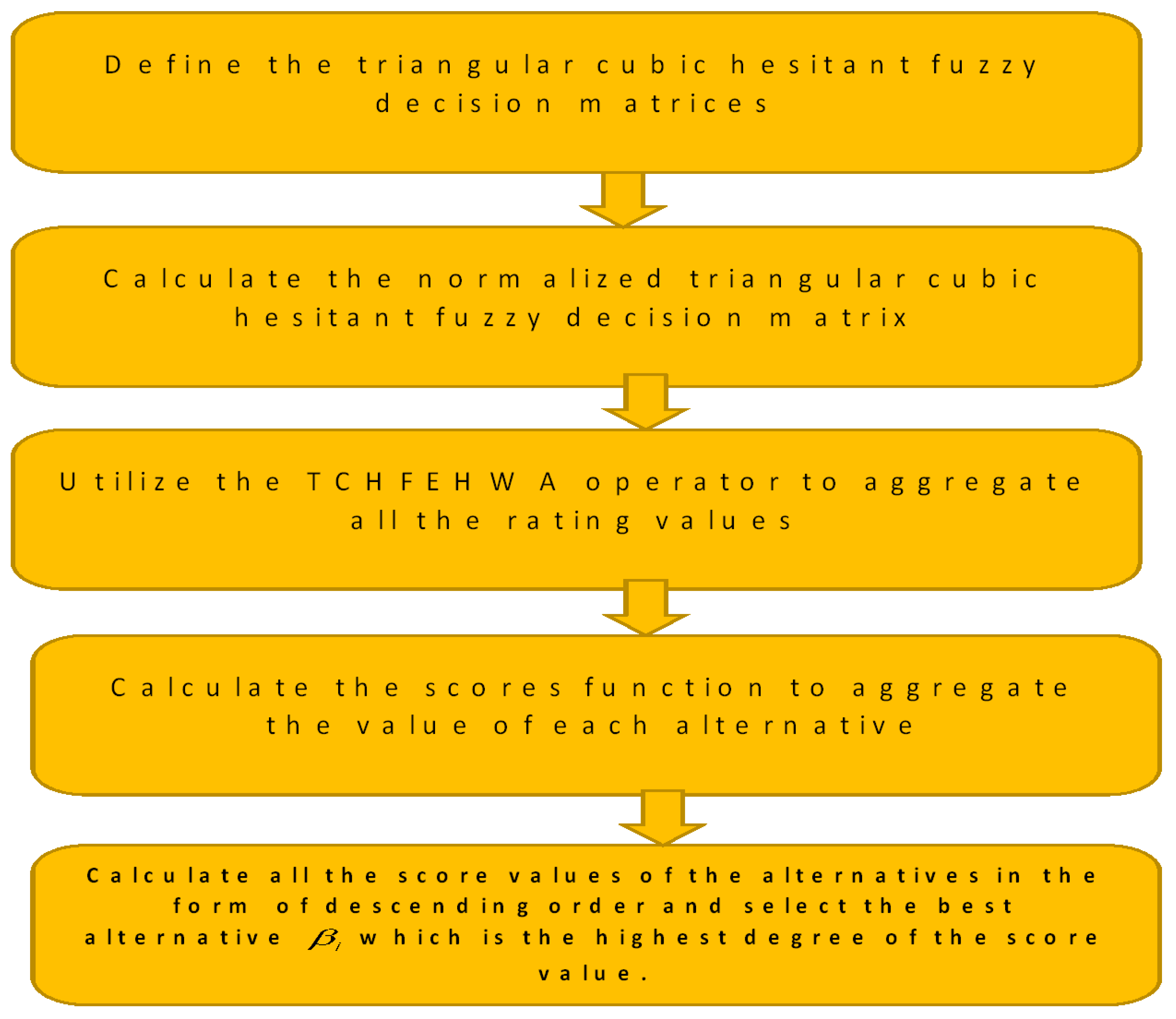
6. An Approach to Multiple Attribute Decision Making with Triangular Cubic Hesitant Fuzzy Information

In this section, we shall utilize the triangular cubic hesitant fuzzy operator to multiple attribute decision making with linguistic information.

There are different factors affecting the chain of command in a program, such as the geographical location of projects, the capability of the engineers, staff, and workers, and the similarity of projects comprising the program. Other factors of much importance in constructing a program are the complexity of the projects, the level of the design, the availability of resources, and the technical know-how. In terms of program organization, delegation is very important to keep a tight control over a large number of projects comprising the program.

Alcantud et al. [37] developed two real implementations: (i) new metarankings of world academic institutions that build on real data from three reputed agencies, and (ii) a new procedure for improving teaching performance assessments which we illustrate with real data collected by ourselves.

Author(s)	Tool(s)/method(s)
Based on HFEs scores
Xia and Xu [11]	Generalized hesitant fuzzy weighted averaging operator (GHFWA),
	Generalized hesitant fuzzy weighted geometric operator (GHFWG)
Farhadinia [38]	Series of score functions for hesitant fuzzy sets
Xia, Xu and Zhu [39]	Weighted hesitant fuzzy geometric Bonferroni mean (WHFGBM)
	Weighted hesitant fuzzy Choquet geometric Bonferroni mean (WHFCGBM)
Wei [40]	Hesitant fuzzy prioritized operators

Based on distance measures
Xu and Xia [41]	Distance measures of hesitant fuzzy elements
Xu and Xia [42]	Generalized hesitant weighted distance
Li, Zeng and Li [43]	Distance and similarity measures considering hesitancy degree

A multiple attribute decision making (MADM) problem is to find the best compromise solution from all feasible alternatives assessed on multiple attributes. Let $\stackrel{⃛}{z}=\{{\stackrel{⃛}{z}}_1,{\stackrel{⃛}{z}}_2,\dots ,{\stackrel{⃛}{z}}_n\}$ be a set of alternatives and $G=\{g_1,g_2,\dots ,g_n\}$ be the set of attributes. Suppose the rating of alternatives ${\stackrel{⃛}{z}}_i$$(i=1,2,\dots ,n)$ on attributes $g_j$$(j=1,2,\dots ,m)$ given by decision maker are TCHFNs in $L_{TCHFN}$: $\ddot{A}=〈\begin{array}{c}[a_{\ddot{A}}^{-}(\stackrel{⃛}{z}),b_{\ddot{A}}^{-}(\stackrel{⃛}{z}),c_{\ddot{A}}^{-}(\stackrel{⃛}{z})],\\ a_{\ddot{A}}^{+}(\stackrel{⃛}{z}),b_{\ddot{A}}^{-}(\stackrel{⃛}{z}),c_{\ddot{A}}^{+}(\stackrel{⃛}{z})],\\ a_{\ddot{A}}(\stackrel{⃛}{z}),b_{\ddot{A}}(\stackrel{⃛}{z}),c_{\ddot{A}}(\stackrel{⃛}{z})]\\ |\stackrel{⃛}{z}\in Z\end{array}〉$, where $〈\begin{array}{c}[a_{\ddot{A}}^{-}(\stackrel{⃛}{z}),b_{\ddot{A}}^{-}(\stackrel{⃛}{z}),c_{\ddot{A}}^{-}(\stackrel{⃛}{z})],\\ a_{\ddot{A}}^{+}(\stackrel{⃛}{z}),b_{\ddot{A}}^{+}(\stackrel{⃛}{z}),c_{\ddot{A}}^{+}(\stackrel{⃛}{z})],\end{array}〉$ indicates the interval value triangular hesitant fuzzy number that the alternative ${\stackrel{⃛}{z}}_i$ satisfies the attribute $g_j$ and $〈[p_{\ddot{A}}(\stackrel{⃛}{z}),q_{\ddot{A}}(\stackrel{⃛}{z}),r_{\ddot{A}}(\stackrel{⃛}{z})]〉$ indicates the triangular hesitant fuzzy number that the alternative ${\stackrel{⃛}{z}}_i$ does not satisfy the attribute $g_j$, such that, an MADM problem can be concisely expressed in the triangular cubic hesitant fuzzy decision matrix $\stackrel{⃛}{D}={({\ddot{A}}_{ij})}_{m\times n}=〈\begin{array}{c}[a_{\ddot{A}}^{-}(\stackrel{⃛}{z}),b_{\ddot{A}}^{-}(\stackrel{⃛}{z}),c_{\ddot{A}}^{-}(\stackrel{⃛}{z})],\\ a_{\ddot{A}}^{+}(\stackrel{⃛}{z}),b_{\ddot{A}}^{-}(\stackrel{⃛}{z}),c_{\ddot{A}}^{+}(\stackrel{⃛}{z})],\\ a_{\ddot{A}}(\stackrel{⃛}{z}),b_{\ddot{A}}(\stackrel{⃛}{z}),c_{\ddot{A}}(\stackrel{⃛}{z})]\\ |\stackrel{⃛}{z}\in Z\end{array}〉$.

Then, we utilize the triangular cubic hesitant fuzzy number to develop an approach to multiple attribute decision-making problems with linguistic information, which can be described as following:

Step 1: Define the triangular cubic hesitant fuzzy decision matrix

Step 2: Calculate the normalized triangular cubic hesitant fuzzy decision matrix. The following normalization formula $E^k={({\ddot{\beta }}_{ij}^k)}_{n\times 1},$

Accordingly, we attain the normalized triangular cubic hesitant fuzzy decision matrix $\stackrel{⃜}{E}={({\ddot{\beta }}_{ij})}_{n\times m}$.

Step 3: Utilize the TCHFEHWA operator to aggregate all the rating values ${\ddot{\beta }}_{ij}$$(j=1,2,\dots ,m)$ of the ith line and get the overall rating value ${\ddot{\beta }}_{ij}$ corresponding to the alternative ${\stackrel{⃛}{z}}_i$$(i=1,2,\dots ,n),$ i.e., ${\ddot{\beta }}_{ij}$ = TCHFHWA$({\ddot{\beta }}_{i1},{\ddot{\beta }}_{i2},\dots ,{\ddot{\beta }}_{im})=$

$$〈\begin{array}{c}\underset{p^{-}\in a^{-},q^{-}\in b^{-},r^{-}\in c^{-}}{\cup }\left[\begin{array}{c}\frac{{\displaystyle \prod _{i=1}^n}{[1+p_i^{-}(\stackrel{⃛}{z})]}^{\ddot{\omega }}-{\displaystyle \prod _{i=1}^n}{[1-p_i^{-}(\stackrel{⃛}{z})]}^{\ddot{\omega }}}{{\displaystyle \prod _{i=1}^n}{[1+p_i^{-}(\stackrel{⃛}{z})]}^{\ddot{\omega }}+{\displaystyle \prod _{i=1}^n}{[1-p_i^{-}(\stackrel{⃛}{z})]}^{\ddot{\omega }}},\frac{{\displaystyle \prod _{i=1}^n}{[1+q_i^{-}(\stackrel{⃛}{z})]}^{\ddot{\omega }}-{\displaystyle \prod _{i=1}^n}{[1-q_i^{-}(\stackrel{⃛}{z})]}^{\ddot{\omega }}}{{\displaystyle \prod _{i=1}^n}{[1+q_i^{-}(\stackrel{⃛}{z})]}^{\ddot{\omega }}+{\displaystyle \prod _{i=1}^n}{[1-q_i^{-}(\stackrel{⃛}{z})]}^{\ddot{\omega }}},\\ \frac{{\displaystyle \prod _{i=1}^n}{[1+r_i^{-}(\stackrel{⃛}{z})]}^{\ddot{\omega }}-{\displaystyle \prod _{i=1}^n}{[1-r_i^{-}(\stackrel{⃛}{z})]}^{\ddot{\omega }}}{{\displaystyle \prod _{i=1}^n}{[1+r_i^{-}(\stackrel{⃛}{z})]}^{\ddot{\omega }}+{\displaystyle \prod _{i=1}^n}{[1-r_i^{-}(\stackrel{⃛}{z})]}^{\ddot{\omega }}}\end{array}\right],\\ \underset{p^{+}\in a^{+},q^{+}\in b^{+},r^{+}\in c^{+}}{\cup }\left[\begin{array}{c}\frac{{\displaystyle \prod _{i=1}^n}{[1+p_i^{+}(\stackrel{⃛}{z})]}^{\ddot{\omega }}-{\displaystyle \prod _{i=1}^n}{[1-p_i^{+}(\stackrel{⃛}{z})]}^{\ddot{\omega }}}{{\displaystyle \prod _{i=1}^n}{[1+p_i^{+}(\stackrel{⃛}{z})]}^{\ddot{\omega }}+{\displaystyle \prod _{i=1}^n}{[1-p_i^{+}(\stackrel{⃛}{z})]}^{\ddot{\omega }}},\frac{{\displaystyle \prod _{i=1}^n}{[1+q_i^{+}(\stackrel{⃛}{z})]}^{\ddot{\omega }}-{\displaystyle \prod _{i=1}^n}{[1-q_i^{+}(\stackrel{⃛}{z})]}^{\ddot{\omega }}}{{\displaystyle \prod _{i=1}^n}{[1+q_i^{+}(\stackrel{⃛}{z})]}^{\ddot{\omega }}+{\displaystyle \prod _{i=1}^n}{[1-q_i^{+}(\stackrel{⃛}{z})]}^{\ddot{\omega }}},\\ \frac{{\displaystyle \prod _{i=1}^n}{[1+r_i^{+}(\stackrel{⃛}{z})]}^{\ddot{\omega }}-{\displaystyle \prod _{i=1}^n}{[1-r_i^{+}(\stackrel{⃛}{z})]}^{\ddot{\omega }}}{{\displaystyle \prod _{i=1}^n}{[1+r_i^{+}(\stackrel{⃛}{z})]}^{\ddot{\omega }}+{\displaystyle \prod _{i=1}^n}{[1-r_i^{+}(\stackrel{⃛}{z})]}^{\ddot{\omega }}}\end{array}\right],\\ \underset{\begin{array}{c}p\in a,q\in b,r\in c\end{array}}{\cup }\left[\begin{array}{c}\frac{2{\displaystyle \prod _{i=1}^n}{[p_i(\stackrel{⃛}{z})]}^{\ddot{\omega }}}{{\displaystyle \prod _{i=1}^n}[{(2-p_i(\stackrel{⃛}{z})]}^{\ddot{\omega }}+{\displaystyle \prod _{i=1}^n}{[p_i(\stackrel{⃛}{z})]}^{\ddot{\omega }}},\frac{2{\displaystyle \prod _{i=1}^n}{[q_i(\stackrel{⃛}{z})]}^{\ddot{\omega }}}{{\displaystyle \prod _{i=1}^n}[{(2-q_i(\stackrel{⃛}{z})]}^{\ddot{\omega }}+{\displaystyle \prod _{i=1}^n}{[q_i(\stackrel{⃛}{z})]}^{\ddot{\omega }}},\\ \frac{2{\displaystyle \prod _{i=1}^n}{[r_i(\stackrel{⃛}{z})]}^{\ddot{\omega }}}{{\displaystyle \prod _{i=1}^n}[{(2-r_i(\stackrel{⃛}{z})]}^{\ddot{\omega }}+{\displaystyle \prod _{i=1}^n}{[r_i(\stackrel{⃛}{z})]}^{\ddot{\omega }}}\end{array}\right]\end{array}〉$$

(16)

where $\ddot{\omega }$ $={({\ddot{\omega }}_1,{\ddot{\omega }}_2,\dots ,{\ddot{\omega }}_n)}^T$ is the attribute weight vector of $g_j$$(j=1,2,\dots ,m)$ such that ${\ddot{\omega }}_j\in [0,1]$, $(j=1,2,\dots ,m)$ and ${\displaystyle \sum _{j=1}^n}{\ddot{\omega }}_j$ $=1.$ $w={(w_1,w_2,\dots ,w_n)}^T$ is the associated vector of the TCHFEHWA operator, such that $w_j\in [0,1],j=1,2,\dots ,n$ and ${\displaystyle \sum _{j=1}^n}{w}_j=1.$

${\ddot{\beta }}_{ij}$ = TCHFHWA$({\ddot{\beta }}_{j1},{\ddot{\beta }}_{j2},\dots ,{\ddot{\beta }}_{jm})=$ $〈\begin{array}{c}\underset{p^{-}\in a^{-},q^{-}\in b^{-},r^{-}\in c^{-}}{\cup }[\frac{{\displaystyle \prod _{j=1}^n}{[1+p_{\sigma (j)}^{-}]}^{\varpi }-{\displaystyle \prod _{j=1}^n}{[1-p_{\sigma (j)}^{-}]}^{\varpi }}{{\displaystyle \prod _{j=1}^n}{[1+p_{\sigma (j)}^{-}]}^{\varpi }+{\displaystyle \prod _{j=1}^n}{[1-p_{\sigma (j)}^{-}]}^{\varpi }},\frac{{\displaystyle \prod _{j=1}^n}{[1+q_{\sigma (j)}^{-}]}^{\varpi }-{\displaystyle \prod _{j=1}^n}{[1-q_{\sigma (j)}^{-}]}^{\varpi }}{{\displaystyle \prod _{j=1}^n}{[1+q_{\sigma (j)}^{-}]}^{\varpi }+{\displaystyle \prod _{j=1}^n}{[1-q_{\sigma (j)}^{-}]}^{\varpi }},\\ \frac{{\displaystyle \prod _{j=1}^n}{[1+r_{\sigma (j)}^{-}]}^{\varpi }-{\displaystyle \prod _{j=1}^n}{[1-r_{\sigma (j)}^{-}]}^{\varpi }}{{\displaystyle \prod _{j=1}^n}{[1+r_{\sigma (j)}^{-}]}^{\varpi }+{\displaystyle \prod _{j=1}^n}{[1-r_{\sigma (j)}^{-}]}^{\varpi }}],\underset{p^{+}\in a^{+},q^{+}\in b^{+},r^{+}\in c^{+}}{\cup }[\frac{{\displaystyle \prod _{j=1}^n}{[1+p_{\sigma (j)}^{+}]}^{\varpi }-{\displaystyle \prod _{j=1}^n}{[1-p_{\sigma (j)}^{+}]}^{\varpi }}{{\displaystyle \prod _{j=1}^n}{[1+p_{\sigma (j)}^{+}]}^{\varpi }+{\displaystyle \prod _{j=1}^n}{[1-p_{\sigma (j)}^{+}]}^{\varpi }},\\ \frac{{\displaystyle \prod _{j=1}^n}{[1+q_{\sigma (j)}^{+}]}^{\varpi }-{\displaystyle \prod _{j=1}^n}{[1-q_{\sigma (j)}^{+}]}^{\varpi }}{{\displaystyle \prod _{j=1}^n}{[1+q_{\sigma (j)}^{+}]}^{\varpi }+{\displaystyle \prod _{j=1}^n}{[1-q_{\sigma (j)}^{+}]}^{\varpi }},\frac{{\displaystyle \prod _{j=1}^n}{[1+r_{\sigma (j)}^{+}]}^{\varpi }-{\displaystyle \prod _{j=1}^n}{[1-r_{\sigma (j)}^{+}]}^{\varpi }}{{\displaystyle \prod _{j=1}^n}{[1+r_{\sigma (j)}^{+}]}^{\varpi }+{\displaystyle \prod _{j=1}^n}{[1-r_{\sigma (j)}^{+}]}^{\varpi }}\\ \underset{\begin{array}{c}p\in a,q\in b,r\in c\end{array}}{\cup }\left[\begin{array}{c}\frac{2{\displaystyle \prod _{j=1}^n}{[p_{\sigma (j)}]}^{\varpi }}{{\displaystyle \prod _{j=1}^n}[{(2-p_{\sigma (j)}]}^{\varpi }+{\displaystyle \prod _{j=1}^n}{[p_{\sigma (j)}]}^{\varpi }},\frac{2{\displaystyle \prod _{j=1}^n}{[q_{\sigma (j)}]}^{\varpi }}{{\displaystyle \prod _{j=1}^n}[{(2-q_{\sigma (j)}]}^{\varpi }+{\displaystyle \prod _{j=1}^n}{[q_{\sigma (j)}]}^{\varpi }},\\ \frac{2{\displaystyle \prod _{j=1}^n}{[r_{\sigma (j)}]}^{\varpi }}{{\displaystyle \prod _{j=1}^n}[{(2-r_{\sigma (j)}]}^{\varpi }+{\displaystyle \prod _{j=1}^n}{[r_{\sigma (j)}]}^{\varpi }}\end{array}\right]\end{array}〉$

Step 4: Calculate the scores function to aggregate the value of each alternative ${\ddot{\beta }}_i$$(i=1,2,\dots ,n)$, then we have must find out the score value of the aggregate value of each alternative.

Step 5: Calculate all the score values of the alternatives in the form of descending order and select the best alternative ${\ddot{\beta }}_i$ which is the highest degree of the score value.

Next, we shall apply the TCHFEHWA operator to deal with the MADM problem, which involves the following algorithm steps.

Algorithm. A MAGDM approach based on the triangular cubic hesitant fuzzy number

Output: The Ranking of all the alternatives

Step 1: Define the triangular cubic hesitant fuzzy matrix

Step 2: Calculate the normalized triangular cubic hesitant fuzzy decision matrix to obtain the integrated information by aggregating individual information for all DMs.

Step 3: Utilize the TCHFEHWA operator to aggregate all the rating values ${\ddot{\beta }}_{ij}$$(j=1,2,\dots ,m)$ of the ith line and get the overall rating value ${\ddot{\beta }}_{ij}$ corresponding to the alternative ${\stackrel{⃛}{z}}_i$$(i=1,2,\dots ,n).$

Step 4: Calculate the scores function based on the (Eq. 4) of each alternative ${\ddot{\beta }}_i$$(i=1,2,\dots ,n)$, then we have must find out the score value of the aggregate value of each alternative.

Step 5: Rank all the alternatives in the form of descending order and select the best alternative ${\ddot{\beta }}_i$ which is the highest degree of the score value.

Figure 2 is a flow chart describing the steps of the algorithm.

7. Illustrative Example

Regular exposures and disasters are yonder gentleman’s controller. Whatever can take the defensive events before its incidence or can ensure less injury by expressing an efficient disaster administration strategy so as to evade loss of humanoid life and additional essential resources is unique. Consider Pakistan where deluges hit numerous conditions and principal to vast loss of life and stuff. Directing on the disaster management, related particularly to four Indian States, taken as alternatives $A_i,i=1,2,3,$ viz., (Lahore, Mansehra, and Islamabad) which remained largely devastated during first half of the year 2018, suppose the Administration of Pakistan is trying to make the best decision on allocating reserves to these three conditions. When the whole situation is examined for major areas of fund allocation, it was found that money should be allocated in such a way that three major factors represented by $C_j,j=1,2,3$ namely: “Food Shortage”, “Amount of persons saved” and “Absence of substructure Rebuilding amenities” needed to be coped up. Suppose, different factors are prioritized state-wise in accordance with the weight vector $\ddot{\omega }=(0.25,0.50,0.25)$. Thus, the aim of the problem is to determine the order in which states should be allocated the relief fund.

It ends with a discussion on how to aggregate information that is expressed in terms of linguistic variables. This is a crucial step of the process of decision making, as we need to be able to aggregate the various bits of “linguistic” information (that is expressed in linguistic format) on the issue at hand under the condition of fulfilling certain criteria. The following section then explicates how to model the decision-making process in various succeeding stages. One way to avoid the above problems associated with using membership functions is to use linguistic variables instead of fuzzy numbers, that is, to use variables whose values are not numbers but words or sentences in a natural or artificial language. Since words are in general less precise than numbers, the concept of a linguistic variable serves the purpose of providing a means to approximately characterize phenomena that are complex or ill-defined and hence not amenable to a crisp description in quantitative terms. Of course, in order for linguistic variables to be useful tools of analysis, one ought to be able to manipulate them through various operations. Generally, manipulating linguistic variables can be done in one of two ways. First, one can use linguistic variables by associating membership functions to them and then manipulating the membership functions, since linguistic variables are but a special category of fuzzy sets. Second, one can directly symbolically manipulate the linguistic variables themselves.

In the former case, the manipulation of linguistic variables is done by using the extension principle, which in essence allows the extension of usual algebraic and arithmetic manipulations to fuzzy sets. However, using extended arithmetic operations to handle fuzzy numbers increases the vagueness of results at every step of the calculation, and the shape of the membership functions is not preserved. The final results of this kind of method are fuzzy sets with membership functions that are often hard to interpret, thereby making the corresponding final linguistic variables outside the original set of linguistic terms that one starts from. In the second approach, based on using algebraic operations on the linguistic variables themselves, there is no need to manipulate any sort of membership functions at all. In the following, a summary of the contours of the symbolic approach is presented. The approach is introduced and illustrated by discussing a hypothetical situation in which state leaders have to make choices on how to build a security alignment. This is a fictitious example, hence there is no attempt to justify the posited underlying substantive assumptions for why certain variables are chosen.

The linguistic fuzzy analysis is mathematically rigorous, that is, it is built on a coherent mathematical framework of definitions, theorems, lemmas, and the like. A key idea behind this approach is to directly manipulate the available linguistic information and knowledge. In this pursuit, the first step is to choose the basic ingredients that are used in the symbolic manipulation. This means that the analyst has to choose a context-dependent linguistic term set to describe vague or imprecise information. For example, linguistic terms set for the linguistic variable Importance denoted by H(Importance), can be defined as H(Importance) $=$ {important, not important, very important, not very important, fairly important}. Normally, in any one situation of a decision under multiple criteria, one is faced with a number of linguistic variables, not just one. It is easier to opt for the same linguistic terms set to describe a variation of the various linguistic concepts in the problem at hand, although this is not a requirement. The elements in the set will determine the level of distinction among different parts of the available information, called the granularity of uncertainty. Each value of the linguistic variables is characterized by a syntactic label and a semantic value or meaning. The label is a word or a sentence belonging to the chosen linguistic terms set. The meaning of the label is a fuzzy subset in a universe of discourse (a finite set of words and phrases). The choice of the linguistic terms set with its semantic is thus the first step of any linguistic approach to solving a problem.

Assume that the decision-maker procedures the linguistic terms to the evaluating estimates of the alternatives with reverence to different attributes individually as shown in

Table 1. Linguistic terms of triangular cubic hesitant fuzzy values.

. The relationship between the linguistic terms and the comparing TCHFNs in $L_{\mathit{TCHFN}}$ as appeared in

Table 2. Triangular cubic hesitant fuzzy Decision matrix.

and

Table 3. Triangular cubic hesitant fuzzy Decision matrix.

.

Step 1: Define triangular cubic hesitant fuzzy Decision matrix Table 2 and Table 3.

Step 2: Get the normalized triangular cubic hesitant fuzzy decision matrix. The following normalization formula $E^k={({\ddot{\beta }}_{ij}^k)}_{n\times 1}.$ The normalized decision matrix is presented in

Table 4. Normalized decision matrix.

and

Table 5. Normalized decision matrix table.

.

Hence, we acquire the standardized triangular cubic hesitant fuzzy decision matrix $E={({\ddot{\beta }}_{ij})}_{n\times m}$.

Step 3: Utilize the TCHFEHWA operator rating values in

Table 6. Rating value of the TCHFEHWA operator.

and get the general rating value ${\ddot{\beta }}_{ij}$ as displayed in

Table 7. General rating value.

to be compared to the alternative ${\stackrel{⃛}{z}}_i,w=(0.25,0.50,0.25)$.

$w=(0.25,0.25,0.50)$

Step 4: Calculate the scores function to aggregate the value of each alternative ${\ddot{\beta }}_i$$(i=1,2,\dots ,n)$, then we have must to find out the score value of the aggregate value of each alternative. ${\ddot{s}}_1=\frac{2.2924}{9}=0.2547,{\ddot{s}}_2=\frac{3.2564}{9}=0.3618,{\ddot{s}}_3=\frac{3.6926}{9}=0.4102.$

Step 5: Arrange the scores of all alternatives in the form of descending order and select that alternative which is the highest score function. Since ${\ddot{s}}_3>{\ddot{s}}_2>{\ddot{s}}_1$, thus the most wanted alternative is ${\ddot{s}}_3$.

Figure 3 is the graph illustrating the three ranking.

8. Comparison Analysis

In order to verify the validity and effectiveness of the proposed approach, a comparative study is conducted using the methods of interval-valued intuitionistic hesitant fuzzy number [25] and hesitant triangular intuitionistic fuzzy number [23], which are special cases of TCHFNs, to the same illustrative example.

8.1. A Comparison Analysis of the Existing MCDM Interval-Valued Intuitionistic Hesitant Fuzzy Number with Our Proposed Methods

An interval-valued intuitionistic hesitant fuzzy number can be considered as a special case of triangular cubic hesitant fuzzy numbers when there is the only element in membership and non-membership degree [25]. For comparison, the interval-valued intuitionistic hesitant fuzzy number can be transformed to the triangular cubic hesitant fuzzy number (TCHFN) by calculating the average value of the membership and nonmembership degrees. After transformation, the interval-valued intuitionistic hesitant fuzzy number are given in

Table 8. Interval-valued intuitionistic hesitant fuzzy decision matrix.

and

Table 9. IVIHFWA operator.

.

Step 1: Calculate the interval-valued intuitionistic hesitant fuzzy weighted averaging (IVIHFWA) operator $\omega ={(0.3,0.2,0.5)}^T$.

Step 2: Calculate the score value $s_1=0.1553,s_2=-0.0705,s_3=0.4855.$

Step 3: Rank all the alternatives. According to the ranking of score function $S(z_i)$, the ranking is $s_3>s_1>s_2$.

Figure 4 is the graph illustrating the position of the three scores.

The ranking of all alternatives $s_3>s_1>s_2$ and $s_3$ is the best selection. Obviously, the ranking is derived from the method proposed by Zhang [25], is different from the result of the proposed method. The main reasons are that an interval-valued intuitionistic hesitant fuzzy number only consider the triangular number, membership degrees of an element and nonmembership degrees, which may result in information interval-valued intuitionistic hesitant fuzzy number are not equal.

8.2. A Comparison Analysis of the Existing MCDM Hesitant Triangular Intuitionistic Fuzzy Number with Our Proposed Methods

The hesitant triangular intuitionistic fuzzy number can be considered as a special case of triangular cubic hesitant fuzzy numbers when there is the only element in membership and non-membership degree [23]. For comparison, the hesitant triangular intuitionistic fuzzy number can be transformed into the triangular cubic hesitant fuzzy number (TCHFN) by calculating the average value of the membership and nonmembership degrees. After transformation, the hesitant triangular intuitionistic fuzzy number are given in

Table 10. Hesitant triangular intuitionistic fuzzy decision matrix.

and

Table 11. HTIFWG operator.

.

Step 1: Calculate the Hesitant triangular intutionistic fuzzy weighted geometric (HTIFWG) opeator $\omega ={(0.3,0.2,0.5)}^T$.

Step 2: Calculate the score value $s_1=0.0165,s_2=0.1083,s_3=-0.0279.$

Step 3: Rank all the alternatives. According to the ranking of score function $S(z_i)$, the ranking is $s_2>s_1>s_3$.

Figure 5 is the graph illustrating the position of the three scores. The ranking of all alternatives $s_2>s_1>s_3$ and $s_2$ is the best selection. Obviously, the ranking is derived from the method proposed by Chen et al. [23] in

Table 12. Comparison analysis with existing methods.

, is different from the result of the proposed method. The main reasons are that hesitant triangular intuitionistic fuzzy number only consider the triangular number, membership degrees of an element and nonmembership degrees, which may result in information hesitant triangular intuitionistic fuzzy number are not equal.

The following advantages of our proposal can be summarized on the basis of the above comparison analyses. Triangular cubic hesitant fuzzy number (TCHFN) are very suitable for illustrating uncertain or fuzzy information in MCDM problems because the membership and non-membership degrees can be two sets of several possible values, which cannot be achieved by interval-valued intuitionistic hesitant fuzzy number and intuitionistic triangular hesitant fuzzy number. On the basis of basis operations, aggregation operators and comparison method of triangular cubic hesitant fuzzy number (TCHFN) can be also used to process interval-valued intuitionistic hesitant fuzzy number and intuitionistic triangular hesitant fuzzy number after slight adjustments, because triangular cubic hesitant fuzzy number (TCHFN) can be considered as the generalized form of interval-valued intuitionistic hesitant fuzzy number and intuitionistic triangular hesitant fuzzy number. The defined operations of Triangular cubic hesitant fuzzy number (TCHFN) give us more accurate than the existing operators. This further enhanced the idea of decision making besides the established Q-fuzzy sets [44,45,46] and vague sets [47,48,49].

9. Conclusions

In this paper, we develop the new idea of triangular cubic hesitant fuzzy number and operational laws. We develop the score function S(A), accuracy function H(A), membership uncertainty index T(A) and hesitation uncertainty index G(A). We develop the Einstein operations on Triangular cubic hesitant fuzzy sets. We develop three arithmetic averaging operators, that are triangular cubic hesitant fuzzy Einstein weighted averaging (TCHFEWA) operator, triangular cubic hesitant fuzzy Einstein ordered weighted averaging (TCHFEOWA) operator and triangular cubic hesitant fuzzy Einstein hybrid weighted averaging (TCHFEHWA) operator, for gathering cubic hesitant fuzzy data. The TCHFEHWA operator simplifies both the TCHFEWA and TCHFEOWA operators. Moreover, we apply the developed aggregation operators to multiple attribute group decision-making with triangular cubic hesitant fuzzy information. We apply on the TCHFEHWA operator to multiple attribute decision making with the triangular cubic hesitant fuzzy material. Finally, a numerical example is used to illustrate the validity of the proposed approach in group decision-making problems. The advantages of this new method are that: (1) it is more reliable and reasonable to aggregate the Einstein information under the triangular cubic hesitant fuzzy numbers environment; (2) it offers an effective and powerful mathematics tool for the MADM under uncertainty and can provide more reliable and flexible aggregation results in decision making; (3) it not only considers relationships between the input arguments or the attributes, but also takes into account the correlation between input argument and itself or the interrelations between the attribute and itself, furthermore, interrelationships between input arguments or the attributes are tackled once. The new methods provide some reasonable and reliable MADM aggregation operators, which broaden the selection scope of the decision makers and offer theory Einstein for the MADM methods. In group decision-making problems, because the experts usually come from different speciality fields and have different backgrounds and levels of knowledge, they usually have diverging opinions. Thus, in future work, we will present a consensus model for group decision-making with trapezoidal cubic linguistic neutrosophic hesitant fuzzy information.

References

1. Atanassov, K.T. Intuitionistic fuzzy sets. Fuzzy Sets Syst. 1986, 20, 87–96. [Google Scholar] [CrossRef]
2. Zadeh, L.A. Information and control. Fuzzy Sets 1965, 8, 338–353. [Google Scholar]
3. Zadeh, L.A. Outline of a new approach to analysis of complex systems and decision processes interval-valued fuzzy sets. IEEE Trans. Syst. Man Cybern. SMC 1973, 3, 28–44. [Google Scholar] [CrossRef]
4. Bustince, H.; Burillo, P. Structures on intuitionistic fuzzy relations. Fuzzy Sets Syst. 1996, 78, 293–303. [Google Scholar] [CrossRef]
5. Deschrijver, G.; Kerre, E.E. On the relationship between some extensions of fuzzy set theory. Fuzzy Sets Syst. 2003, 133, 227–235. [Google Scholar] [CrossRef]
6. Deschrijver, G.; Kerre, E.E. On the position of intuitionistic fuzzy set theory in the framework of theories modelling imprecision. Inf. Sci. 2007, 177, 1860–1866. [Google Scholar] [CrossRef]
7. Turksen, I.B. Interval valued fuzzy sets based on normal forms. Fuzzy Sets Syst. 1986, 20, 191–210. [Google Scholar] [CrossRef]
8. Xu, Z. Intuitionistic fuzzy aggregation operators. IEEE Trans. Fuzzy Syst. 2007, 15, 1179–1187. [Google Scholar]
9. Chen, N.; Xu, Z.; Xia, M. Interval-valued hesitant preference relations and their applications to group decision making. Knowl.-Based Syst. 2013, 37, 528–540. [Google Scholar] [CrossRef]
10. Torra, V. Hesitant fuzzy sets. Int. J. Intell. Syst. 2010, 25, 529–539. [Google Scholar] [CrossRef]
11. Xia, M.; Xu, Z. Hesitant fuzzy information aggregation in decision making. Int. J. Approx. Reason. 2011, 52, 395–407. [Google Scholar] [CrossRef] [Green Version]
12. Xia, M.; Xu, Z.; Chen, N. Some hesitant fuzzy aggregation operators with their application in group decision making. Group Decis. Negot. 2013, 22, 259–279. [Google Scholar] [CrossRef]
13. Zeng, S.; Su, W. Intuitionistic fuzzy ordered weighted distance operator. Knowl.-Based Syst. 2011, 24, 1224–1232. [Google Scholar] [CrossRef]
14. Xu, Z.; Yager, R.R. Some geometric aggregation operators based on intuitionistic fuzzy sets. Int. J. Gener. Syst. 2006, 35, 417–433. [Google Scholar] [CrossRef]
15. Xu, Z.; Yager, R.R. Dynamic intuitionistic fuzzy multi-attribute decision making. Int. J. Approx. Reason. 2008, 48, 246–262. [Google Scholar] [CrossRef]
16. Zhao, X.; Lin, R.; Wei, G. Hesitant triangular fuzzy information aggregation based on Einstein operations and their application to multiple attribute decision making. Expert Syst. Appl. 2014, 41, 1086–1094. [Google Scholar] [CrossRef]
17. Lia, J.; Zhang, X.L.; Gong, Z.T. Aggregating of Interval-valued Intuitionistic Uncertain Linguistic Variables based on Archimedean t-norm and It Applications in Group Decision Makings. J. Comput. Anal. Appl. 2018, 24, 874–885. [Google Scholar]
18. Jun, Y.B.; Kim, C.S.; Yang, K.O. Cubic Sets. Ann. Fuzzy Math. Inform. 2011, 4, 83–98. [Google Scholar]
19. Medina, J.; Ojeda-Aciego, M. Multi-adjoint t-concept lattices. Inf. Sci. 2010, 180, 712–725. [Google Scholar] [CrossRef]
20. Pozna, C.; Minculete, N.; Precup, R.E.; Kóczy, L.T.; Ballagi, Á. Signatures: Definitions, operators and applications to fuzzy modelling. Fuzzy Sets Syst. 2012, 201, 86–104. [Google Scholar] [CrossRef]
21. Jankowski, J.; Kazienko, P.; Wątróbski, J.; Lewandowska, A.; Ziemba, P.; Zioło, M. Fuzzy multi-objective modeling of effectiveness and user experience in online advertising. Expert Syst. Appl. 2016, 65, 315–331. [Google Scholar] [CrossRef]
22. Kumar, A.; Kumar, D.; Jarial, S.K. A hybrid clustering method based on improved artificial bee colony and fuzzy C-Means algorithm. Int. J. Artif. Intell. 2017, 15, 24–44. [Google Scholar]
23. Chen, J.; Huang, X. Hesitant Triangular Intuitionistic Fuzzy Information and Its Application to Multi-Attribute Decision Making Problem. J. Nonlinear Sci. Appl. 2017, 10, 1012–1029. [Google Scholar] [CrossRef]
24. Xu, Z.S.; Cai, X. Recent advances in intuitionistic fuzzy information aggregation. Fuzzy Optim. Decis. Mak. 2010, 9, 359–381. [Google Scholar] [CrossRef]
25. Zhang, Z. Interval-Valued Intuitionistic Hesitant Fuzzy Aggregation Operators and Their Application in Group Decision-Making. J. Appl. Math. 2013, 2013, 670285. [Google Scholar] [CrossRef]
26. Fahmi, A.; Abdullah, S.; Amin, F.; Siddique, N.; Ali, A. Aggregation operators on triangular cubic fuzzy numbers and its application to multi-criteria decision making problems. J. Intell. Fuzzy Syst. 2017, 33, 3323–3337. [Google Scholar] [CrossRef]
27. Fahmi, A.; Abdullah, S.; Amin, F.; Ali, A. Precursor Selection for Sol-Gel Synthesis of Titanium Carbide Nanopowders by a New Cubic Fuzzy Multi-Attribute Group Decision-Making Model. J. Intell. Syst. 2017. [Google Scholar] [CrossRef]
28. Fahmi, A.; Abdullah, S.; Amin, F.; Ali, A. Weighted Average Rating (War) Method for Solving Group Decision Making Problem Using Triangular Cubic Fuzzy Hybrid Aggregation (Tcfha). Punjab Univ. J. Math. 2018, 50, 23–34. [Google Scholar]
29. Amin, F.; Fahmi, A.; Abdullah, S.; Ali, A.; Ahmed, R.; Ghanu, F. Triangular cubic linguistic hesitant fuzzy aggregation operators and their application in group decision making. J. Intell. Fuzzy Syst. 2018, 34, 2401–2416. [Google Scholar] [CrossRef]
30. Fahmi, A.; Abdullah, S.; Amin, F. Trapezoidal linguistic cubic hesitant fuzzy topsis method and application to group decision making program. J. New Theory 2017, 19, 27–47. [Google Scholar]
31. Fahmi, A.; Abdullah, S.; Amin, F.; Ali, A.; Khan, W.A. Some geometric operators with Triangular Cubic Linguistic Hesitant Fuzzy number and Their Application in Group Decision-Making. J. Intell. Fuzzy Syst. 2018, 1–15. [Google Scholar] [CrossRef]
32. Fahmi, A.; Abdullah, S.; Amin, F. Expected Values of Aggregation Operators on Cubic Trapezoidal Fuzzy Number and its Application to Multi-Criteria Decision Making Problems. J. New Theory 2018, 22, 51–65. [Google Scholar]
33. Fahmi, A.; Abdullah, S.; Amin, F.; Khan, M.S.A. rapezoidal cubic fuzzy number einstein hybrid weighted averaging operators and its application to decision making. Soft Comput. 2018. [Google Scholar] [CrossRef]
34. Fahmi, A.; Amin, F.; Abdullah, S.; Ali, A. Cubic fuzzy Einstein aggregation operators and its application to decision-making. Int. J. Syst.Sci. 2018, 49, 2385–2397. [Google Scholar] [CrossRef]
35. Amin, F.; Fahmi, A.; Abdullah, S. Dealer using a new trapezoidal cubic hesitant fuzzy TOPSIS method and application to group decision-making program. Soft Comput. 2018, 1–14. [Google Scholar] [CrossRef]
36. Pathinathan, T.; Johnson, S. Trapezoidal hesitant fuzzy multi-attribute decision making based on TOPSIS method. Int. Arch. Appl. Sci. Technol. 2015, 6, 39–49. [Google Scholar]
37. Alcantud, J.C.R.; de Andrés Calle, R.; Torrecillas, M.J.M. Hesitant fuzzy worth: An innovative ranking methodology for hesitant fuzzy subsets. Appl. Soft Comput. 2016, 38, 232–243. [Google Scholar] [CrossRef]
38. Farhadinia, B. A series of score functions for hesitant fuzzy sets. Inf. Sci. 2014, 277, 102–110. [Google Scholar] [CrossRef]
39. Xia, M.; Xu, Z.; Zhu, B. Geometric Bonferroni means with their application in multi-criteria decision making. Knowl.-Based Syst. 2013, 40, 88–100. [Google Scholar] [CrossRef]
40. Wei, G. Hesitant fuzzy prioritized operators and their application to multiple attribute decision making. Knowl.-Based Syst. 2012, 31, 176–182. [Google Scholar] [CrossRef]
41. Xu, Z.; Xia, M. On distance and correlation measures of hesitant fuzzy information. Int. J. Intell. Syst. 2011, 26, 410–425. [Google Scholar] [CrossRef]
42. Xu, Z.; Xia, M. Distance and similarity measures for hesitant fuzzy sets. Inf. Sci. 2011, 181, 2128–2138. [Google Scholar] [CrossRef]
43. Li, D.; Zeng, W.; Li, J. New distance and similarity measures on hesitant fuzzy sets and their applications in multiple criteria decision making. Eng. Appl. Artif. Intell. 2015, 40, 11–16. [Google Scholar] [CrossRef]
44. Adam, F.; Hassan, N. Q-fuzzy soft matrix and its application. AIP Conf. Proc. 2014, 1602, 772–778. [Google Scholar]
45. Adam, F.; Hassan, N. Q-fuzzy soft set. Appl. Math. Sci. 2014, 8, 8689–8695. [Google Scholar] [CrossRef]
46. Adam, F.; Hassan, N. Operations on Q-fuzzy soft set. Appl. Math. Sci. 2014, 8, 8697–8701. [Google Scholar] [CrossRef]
47. Alhazaymeh, K.; Hassan, N. Vague soft set relations and functions. J. Intell. Fuzzy Syst. 2015, 28, 1205–1212. [Google Scholar]
48. Al-Quran, A.; Hassan, N. Neutrosophic vague soft expert set theory. J. Intell. Fuzzy Syst. 2016, 30, 3691–3702. [Google Scholar] [CrossRef]
49. Alhazaymeh, K.; Hassan, N. Mapping on generalized vague soft expert set. Int. J. Pure Appl. Math. 2014, 93, 369–376. [Google Scholar] [CrossRef]
Figure 1. Graph of functions of example 2.
Symmetry 10 00658 g001
Figure 2. Flowchart of the triangular cubic hesitant fuzzy information.
Symmetry 10 00658 g002
Figure 3. Illustration of the ranking.
Symmetry 10 00658 g003
Figure 4. Ranking values in the interval-valued intuitionistic hesitant fuzzy number.
Symmetry 10 00658 g004
Figure 5. Ranking values in the hesitant triangular intuitionistic fuzzy number.
Symmetry 10 00658 g005