Article

Mean-Square Estimation of Nonlinear Functionals via Kalman Filtering

1
Department of Mathematics, Incheon National University, 119 Academy-ro, Yeonsu-gu, Incheon 406-772, Korea
2
Department of Information and Statistics, Research Institute of Natural Science, Gyeongsang National University, 501 Jinjudaero, Jinju, Gyeongsangnam-do 660-701, Korea
3
Laser & Sensor System Team, Hanwha Daejeon Plant, 305 Pangyo-ro, Bundang-gu, Seongnam-si 13488, Korea
*
Author to whom correspondence should be addressed.
Symmetry 2018, 10(11), 630; https://doi.org/10.3390/sym10110630
Submission received: 3 October 2018 / Revised: 2 November 2018 / Accepted: 6 November 2018 / Published: 12 November 2018

Abstract

:
This paper focuses on estimation of a nonlinear functional of state vector (NFS) in discrete-time linear stochastic systems. The NFS represents a nonlinear multivariate functional of state variables, which can indicate useful information of a target system for control. The optimal mean-square estimator of a general NFS represents a function of the Kalman estimate and its error covariance. The polynomial functional of state vector is studied in detail. In this case an optimal estimation algorithm has a closed-form computational procedure. The novel mean-square quadratic estimator is derived. For a general NFS we propose to use the unscented transformation to calculate an optimal estimate. The obtained results are demonstrated on theoretical and practical examples with different types of NFS. Comparative analysis with suboptimal estimators for NFS is presented. The subsequent application of the proposed estimators to linear discrete-time systems demonstrates their practical effectiveness.

1. Introduction

This paper is focused on the development of the optimal mean-square estimator for a nonlinear functional of state vector (NFS) in linear discrete-time stochastic systems. In this section, background material, a concise literature review, the formulation of the problem of interest for this study, the scope and the contributions of this investigation, and the organization of the paper are provided.

1.1. Background and Significance

Kalman filtering and its variations are well-known state estimation techniques in wide use in a variety of applications, such as navigation, target tracking, unmanned vehicle state estimation, communications engineering, air traffic control, biomedical and chemical processing, and many others [1,2,3,4,5,6,7,8,9,10].
However, some applications require the estimation of not only a state vector x t n but also NFS, z t = f ( x t ) , which expresses practical and worthwhile information for control systems. For example, the Euclidean norm, f ( x t ) = x t x t n , represents distance between the current x t and nominal x t n states, respectively.

1.2. Literature Review

The problem of estimation of nonlinear functionals with unknown parameters and signals based on the minimax theory has been studied by many authors [11,12,13,14] and the references therein. Estimation of parameters of nonlinear functional model with known error covariance matrix is presented in [15]. Minimax quadratic estimate for integrated squared derivative of a periodic function is derived in [16]. In [17,18], the optimal matrix of a quadratic functional is determined based on cumulant criteria. Estimation of penalty considered as a quadratic cost functional for a quantum harmonic oscillator is given in [19]. Estimators for integrals of nonlinear functions of a probability density are developed in [20,21]. We also mention estimation of nonlinear functionals of spectral density, periodogram of stationary linear signals [22,23,24]. Some extension of these results is obtained by [25]. In [26] an unknown distance between a target and radar is approximated by Taylor polynomial to subsequent estimation of its coefficients. For algorithms and theory of estimation information measures representing a nonlinear functional of signals the reader is referred to [27,28]. However, most authors have not focused on estimation of nonlinear functionals of vector signals in dynamical models defined by stochastic equations. The first step in this direction is given in [29]. However, main results in [29] are obtained by estimation of an unknown signal with time delays using the robust receding horizon approach, rather than estimation of a nonlinear functional. The current paper focuses on the development of an analytical and computational framework for the optimal mean square estimation of a nonlinear functional, and the original signal is estimated by using the Kalman filter.

1.3. Formulation of the Problem of Interest for this Investigation

Consider a discrete-time linear stochastic system
x k + 1 = F k x k + G k v k ,   k = 0 , 1 , , y k = H k x k + w k ,
where x k n is a state vector, y k m is a measurement vector, the system noise v k q and the measurement noise w k m are uncorrelated white Gaussian noises with zero mean and covariances Q k q × q and R k m × m , respectively, and F k ,   G k , and H k are matrices with compatible dimensions. The initial state, x 0 ~ ( m 0 , C 0 ) , is assumed to be Gaussian and uncorrelated with v k and w k , and m 0 = E ( x 0 ) ,   C 0 = Cov ( x 0 , x 0 ) .
A problem associated with the system portrayed in Equation (1) is that of estimation of the NFS:
z k = f ( x k ) :   n
from the overall noisy sensor measurements Y k = { y 1 , , y k } .

1.4. Scope and Contributions of this Investigation

The aim of this paper is to develop an optimal two-stage minimum mean square error (MMSE) estimator for an arbitrary NFS in a linear stochastic system, and investigate special polynomial and quadratic estimators for which one can obtain important mean square estimation results. The main contributions of the paper are the following:
(1)
This paper studies the MMSE estimation problem of an NFS within the discrete-time Kalman filtering framework. Using the mean square estimation approach, an optimal two-stage nonlinear estimator is proposed.
(2)
The optimal MMSE estimator for polynomial functionals (such as quadratic, cubic and quartic) is derived. We establish that the polynomial estimator representing a compact closed-form formula depends only on the Kalman estimate and its error covariance.
(3)
An important class of quadratic estimators is comprehensively investigated, including derivation of novel matrix equations for the estimated and true mean square error.
(4)
Performance of the proposed estimators for real NFS illustrates their theoretical and practical usefulness.

1.5. Organization of the Paper

This paper is organized as follows. Section 2 presents two motivating examples. The main theoretical results are presented in Section 3, which is divided into four subsections: (i) main idea and general solution; (ii) optimal closed-form MMSE estimator for quadratic functional; (iii) optimal closed-form MMSE estimator for polynomial functional; and, (iv) application of the unscented transformation for estimation of general NFS. Simulation analysis and verification of the proposed estimators are given in Section 4, which is divided into four subsections: (i) estimation of distance between unknown and moving points; (ii) estimation of power and modulus of unknown signal; (iii) estimation of total kinetic energy of wind tunnel system; and, (iv) estimation of size of oil spread contour. In Section 5, the summary of this investigation, the conclusions drawn in this paper, and the future direction of research are provided.

2. Motivating Examples

Two examples illustrate an NFS and how it may be used in practice. The first motivating example of the NFS is kinematic quantities of projectile motion. State vector of an object x 4 , an angle ( θ ) and range ( r ) are shown in Figure 1.
f ( x ) = θ = tan 1 ( x 2 / x 1 ) , f ( x ) = r = x 1 2 + x 2 2 , f ( x ) = | v | = x 3 2 + x 4 2 ,     x 3 = v 1 ,     x 4 = v 2 .
The second example can be an arbitrary quadratic form, f ( x t ) = x t T Ω x t , representing an energy-like function of an object or the Euclidean square distance, f ( x t ) = d 2 ( x t , x t n ) , between the current x t and nominal x t n states, respectively. Mechanical examples of a quadratic form as energy and work are shown in Section 3.2.1. Hence, estimation and prediction of quantities represented by an NFS can be helpful in different applications, such as system control and target tracking.

3. Theoretical Results: Optimal Mean Square Estimator for NFS

3.1. Main Idea and General Solution

The main idea of the proposed optimal estimator includes two stages: the optimal Kalman estimate of a state vector computed at the first stage is nonlinearly transformed at the second stage based on the NFS (2) and the MMSE criterion.
At first, according to the MMSE criterion, the optimal estimate of the state x k represents the conditional mean, i.e., x ^ k = E ( x k | Y k ) . The conditional mean and corresponding error covariance P k = Cov ( e k , e k ) ,   e k = x k x ^ k , are described by the recursive Kalman filter (KF) equations [2,8,9,10]:
x ^ k + 1 = F k x ^ k ,   k = 0 , 1 , ;   x ^ 0 = m 0 , P k + 1 = F k P k F k T + G k Q k G k T ,   P 0 = C 0 , K k + 1 = P k + 1 H k + 1 T ( H k + 1 P k + 1 H k + 1 T + R k + 1 ) 1 , x ^ k + 1 = x ^ k + 1 + K k + 1 ( y k + 1 H k + 1 x ^ k + 1 ) , P k + 1 = ( I n K k + 1 H k + 1 ) P k + 1 .
Next, the optimal mean square estimate of the NFS z k = f ( x k ) based on the overall sensor measurements Y k , also represents a conditional mean:
z ^ k = E ( z k | Y k ) = f ( x ) p k ( x | Y k ) dx ,
where p k ( x | Y k ) = ( x ^ k , P k ) is a multivariate conditional Gaussian probability density function.
Thus, the best estimate in (5) represents the MMSE estimator:
z ^ k = F ( x ^ k , P k ) ,
which depends on the Kalman estimate x ^ k and its error covariance P k determined by the KF Equation (4).
Remark: For the general NFS, z k = f ( x k ) , calculation of the optimal estimate, z ^ k = E ( z k | Y k ) , is reduced to calculation of the multivariate integral (5). The shortcoming of the proposed estimator can be attributed to the impossibility of analytically calculating the integrals (optimal estimate) for an arbitrary class of nonlinear functionals. Analytical calculation of the integrals is possible only in special cases which are considered in Section 3.2.2 and Section 3.3. In these cases, the conditional mean E ( z k | Y k ) can be explicitly calculated in terms of x ^ k and P k , and the best MMSE estimator (5) takes a closed-form.

3.2. Optimal Closed-Form MMSE Estimator for Quadratic Functional

Consider an arbitrary quadratic functional (QF) of a state vector x k n :
z k = f ( x k ) = x k T Ω k x k + a k T x k ,
where Ω k = Ω k T 0 and a k are an arbitrary matrix and vector, respectively.

3.2.1. Examples of Quadratic Functional as Energy and Work

Example 1.
Work done from a moving particle
Consider a particle with mass M and speed υ k = υ ( t k ) , which is moving along the x-axis. Let the particle have a velocity υ k at displacement x k = x ( t k ) . Then current work done, z k = W k , represents a QF such as:
W k = 1 2 M υ k 2 1 2 M υ 0 2 = X k T Ω X k , where X k = [ υ k υ 0 ] ,   Ω = [ M 0 0 M ] .
Example 2.
Energy of a harmonic oscillator
The equation of motion of a harmonic oscillator in a random environment is:
M x ¨ t = kx t + ξ t , or [ x ˙ t υ ˙ t ] = [ 0 1 ω 2 0 ] [ x t υ t ] + [ 0 1 ] ξ t ,
where υ t = x ˙ t ,   ω 2 = k / M , M is the mass, k is the force constant of a spring. White Gaussian noise ξ t is added to represent the random environment.
Let sampling period be Δ t = t k t k 1 1 so that terms of order Δ t 2 can be ignored. Then the discretized model of the harmonic oscillator is approximately:
X k + 1 = [ 1 Δ t ω 2 Δ t 1 ] X k + [ 0 1 ] ξ ˜ k ,   X k = [ x k υ k ] ,
where ξ ˜ k represents discrete white noise.
Then energy, z k = E k , is conserved as:
E k = 1 2 M υ k 2 + 1 2 kx k 2 = 1 2 X k T Ω X k ,   Ω = [ k 0 0 M ] .
Here the potential energy is U k = kx k 2 / 2 .

3.2.2. Closed-Form Quadratic Estimator

In the case of the QF (7) the optimal nonlinear estimate (5) can be explicitly calculated in terms of a state estimate x ^ k and its error covariance P k . Using the formula [30]:
E ( x T Ω x ) = tr [ Ω ( C + mm T ) ] , m = E ( x ) ,   C = Cov ( x , x ) ,
we obtain the optimal mean-square estimate for the QF:
z ^ k opt = E ( x k T Ω k x k + a k T x k | Y k ) = tr [ Ω k ( P k + x ^ k x ^ k T ) ] + a k T x ^ k .
In (12) and (13), tr ( A ) is the trace of a matrix A .
In parallel to the optimal estimate (13) consider a suboptimal estimate of the QF, such as z ^ k sub = f ( x ^ k ) :
z ^ k sub = x ^ k T Ω k x ^ k + a k T x ^ k .

3.2.3. True Mean Square Error for Quadratic Estimators

We compare the estimation accuracy of the optimal and suboptimal quadratic estimators (13) and (14), respectively.
The following theorem defines the true mean square errors (MSEs):
P z , k opt = E [ ( z k z ^ k opt ) 2 ] , P z , k sub = E [ ( z k z ^ k sub ) 2 ] .
Theorem 1.
The mean square errors P z , k opt and P z , k sub for the optimal and suboptimal quadratic estimators (13) and (14) are given by:
P z , k opt = 4 tr ( Ω k P k Ω k C k ) 2 tr ( Ω k P k Ω k P k ) + 4 μ k T Ω k P k Ω k μ k + a k T P k a k + 4 μ k T Ω k P k a k ,
and
P z , k sub = 4 tr ( Ω k P k Ω k C k ) 2 tr ( Ω k P k Ω k P k ) + 4 μ k T Ω k P k Ω k μ k + tr 2 ( Ω τ P τ ) + a k T P k a k + 4 μ k T Ω k P k a k ,
respectively. Here the mean μ k = E ( x k ) and covariance C k = Cov ( x k , x k ) are determined by the Lyapunov equation:
μ k + 1 = F k μ k ,   k = 0 , 1 , ;   μ 0 = m 0 = E ( x 0 ) , C k + 1 = F k C k F k T + G k Q k G k T ,   C 0 = Cov ( x 0 , x 0 ) .
The proof of the theorem is given in the Appendix A.
Corollary 1.
In the particular case with z k = x k 2 = x k T x k , the optimal and suboptimal quadratic estimators and MSEs take the form:
z ^ k o p t = tr ( P k + x ^ k x ^ k T ) = x ^ k T x ^ k + t r ( P k ) , z ^ k s u b = x ^ k T x ^ k , P z , k o p t = 4 t r ( P k C k ) 2 t r ( P k 2 ) + 4 μ k T P k μ k , P z , k s u b = 4 t r ( P k C k ) t r ( P k 2 ) + 4 μ k T P k μ k .
Generalization of a QF is a multivariate polynomial functional, which we consider in the next section.

3.3. Optimal Closed-Form MMSE Estimator for Polynomial Functional

Here we consider a special NFS which represents an arbitrary multivariate polynomial functional of an Nth degree:
z k = f ( x k ) = 0 1 + + n N A 1 2 n x 1 , k 1 x 2 , k 2 x n , k n , 1 , 2 , , n = 0 , 1 , , N ,
where A 1 2 n are a nonzero coefficients.
Further for simplicity, we ignore the subscript k of x k , x ^ k ,   x i , k , x ^ i , k and P k ,   P ij , k . In case of the polynomial functional (20), the MMSE estimator, z ^ k = E [ f ( x ) | Y k ] , has a closed form because the best estimate (conditional expectation)
z ^ k = E [ f ( x ) | Y k ] = 0 1 + + n N A 1 2 n E ( x 1 1 x 2 2 x n n | Y k ) ,
depends on high-order conditional moments, m 1 2 n = E ( x 1 1 x 2 2 x n n | Y k ) , of a multivariate Gaussian distribution, which can be explicitly calculated in terms of first- and second-order conditional moments, namely, the Kalman estimate and its error covariance ( x ^ , P ) [31,32]. For example, the third- and fourth-order moments of the components x i of a state vector x T = [ x 1 x n ] are:
E ( x i | Y k ) = x ^ i , E ( x i x j | Y k ) = x ^ i x ^ j + P i j ,   E ( x i x j x | Y k ) = x ^ i x ^ j x ^ + x ^ i P j + x ^ j P i + x ^ P i j , E ( x i x j x h x | Y k ) = x ^ i x ^ j x ^ h x ^ + P i j P h + P i h P j     + P i P j h + x ^ i x ^ j P h + x ^ i x ^ h P j + x ^ i x ^ P j h     + x ^ j x ^ h P i + x ^ j x ^ P i h + x ^ h x ^ P i j , where x ^ T = [ x ^ 1 x ^ n ] ,       P = [ P i j ] ,       i , j = 1 , , n .
For an arbitrary NFS, z k = f ( x k ) , we can use a truncated Taylor series. Then an optimal estimate of NFS can be approximately evaluated using the analytical Equation (22) for high-order moments. Also, to avoid complicated calculations of the multivariate integral in (5) it is useful to apply the unscented transformation.

3.4. Application of Unscented Transformation for Estimation of General NFS

The unscented transformation (UT) approximates the statistics of a transformed random variable, for example, the mean and covariance [33]. Following this approach, the procedure to calculate the best estimate of an NFS, z ^ k opt = E [ f ( x k ) | Y k ] , using the UT can be summarized as follows:
z ^ k opt z ^ k UT = s = 0 2 n ω ( s ) f ( X k ( s ) )
where the sigma points X k ( s ) and corresponding weights ω k ( s ) are determined by:
X k ( 0 ) = x ^ k ,   X k ( s ) = x ^ k + [ ( n + ) P k ] s , X k ( s + n ) = x ^ k [ ( n + ) P k ] s ,   ω ( 0 ) = n + ,   ω ( s ) = ω ( s + n ) = 1 2 ( n + ) ,   s = 1 , , n .
Here [ P k ] s is the sth column of the matrix square root of P k , and is the scaling parameter [34]. Thus, the UT estimate z ^ k UT is represented by known functional of the Kalman estimate x ^ k and error covariance P k .

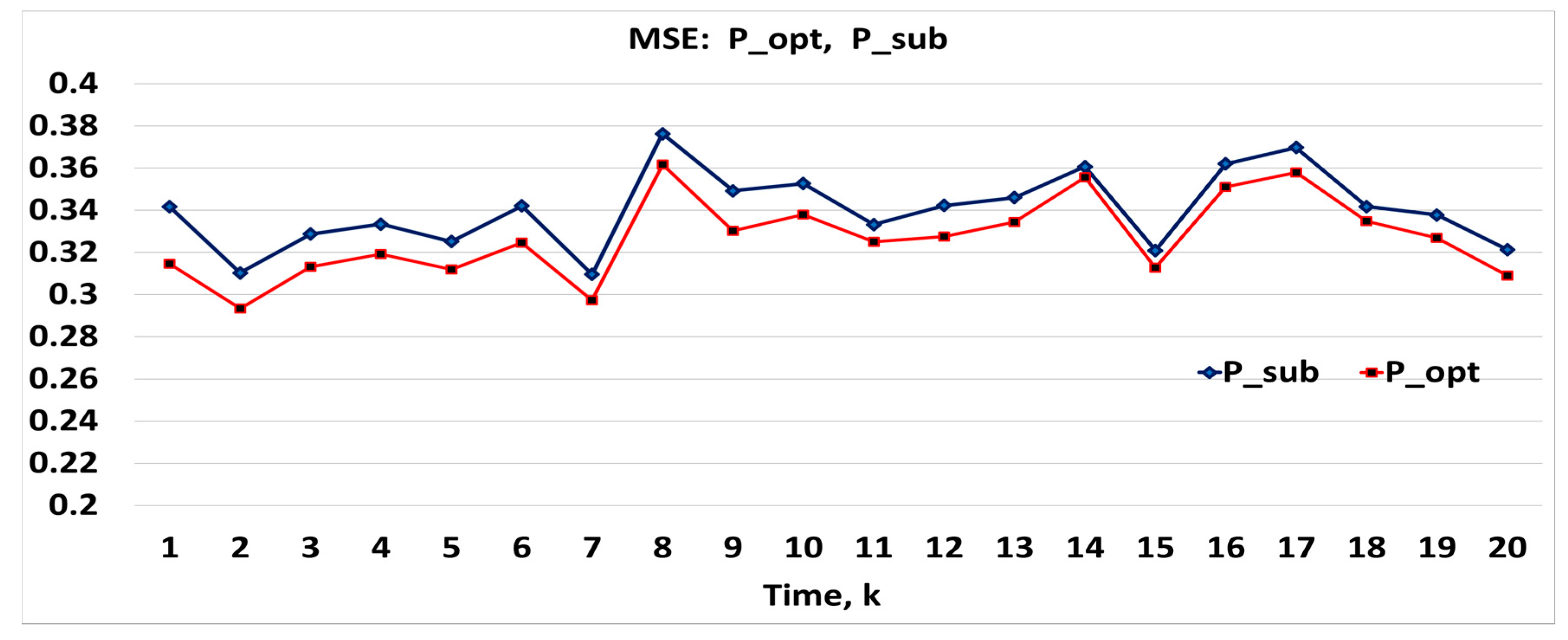
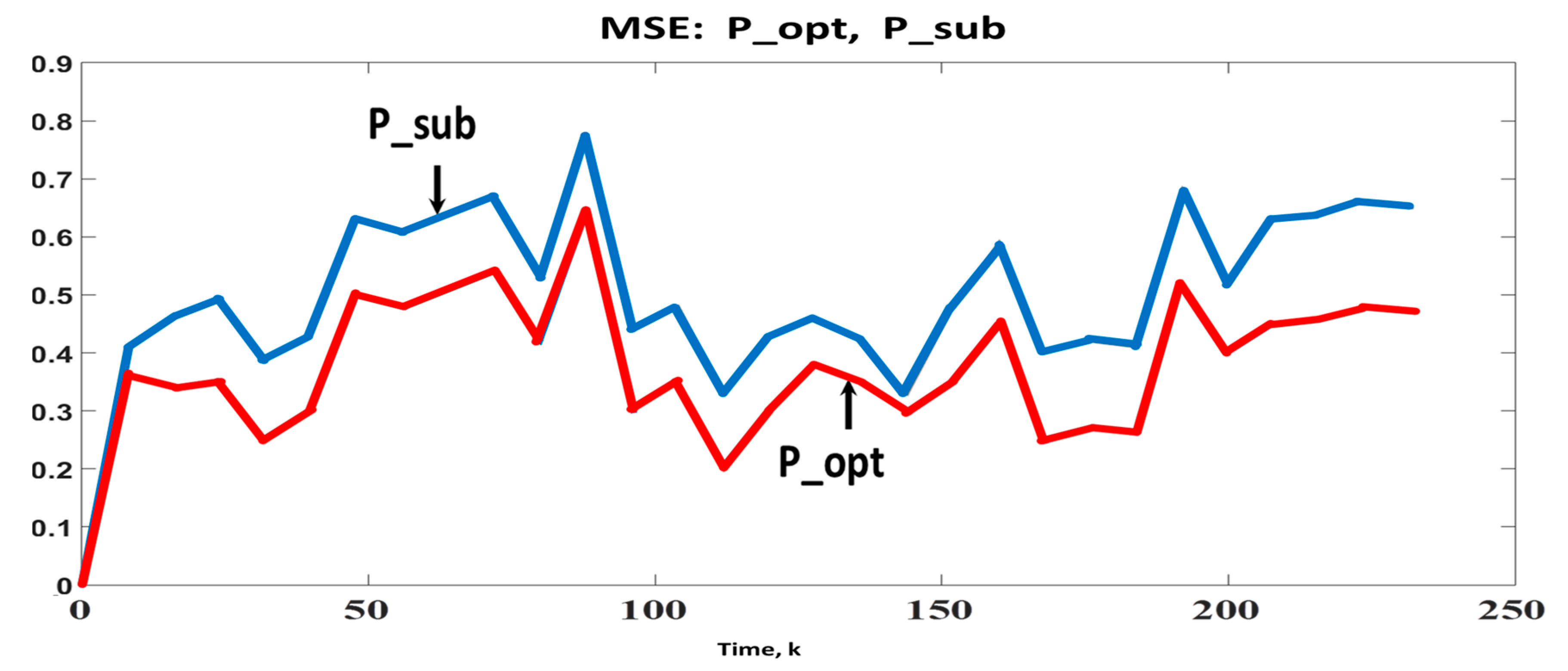
4. Numerical Verification

In this section, demonstrative examples are used for testing the effectiveness of the MMSE estimators developed in this paper.

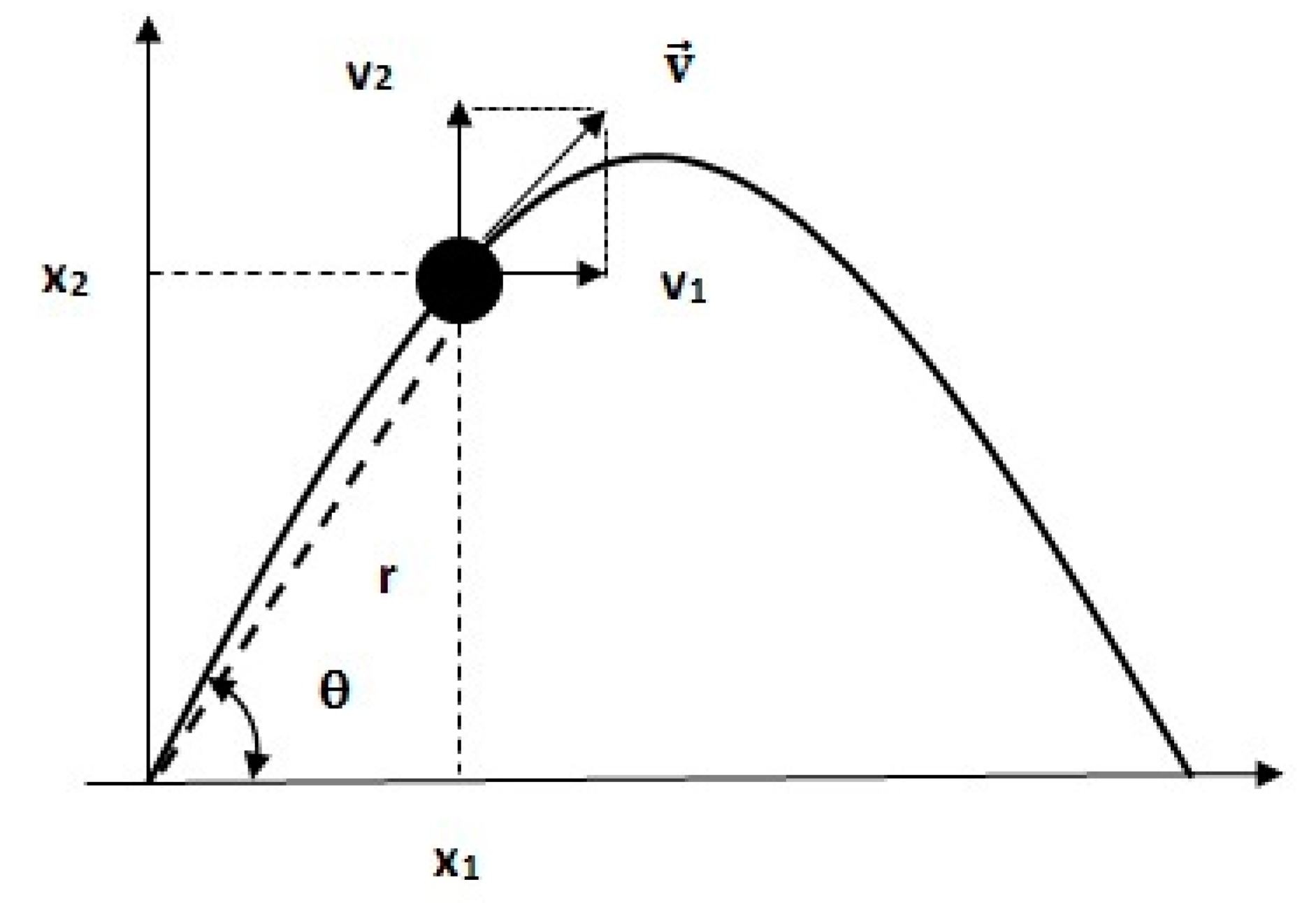
4.1. Estimation of Distance between Unknown and Moving Points

If θ is a scalar unknown which is measured in the presence of additive white noise then:
x k + 1 = x k ,   k = 0 , 1 , ,   x 0 θ ~ ( θ ¯ , σ θ 2 ) , y k = x k + w k ,   w k ~ ( 0 , r ) .
The KF Equation (4) becomes:
x ^ k + 1 = x ^ k + K k + 1 ( y k + 1 x ^ k ) , x ^ 0 = θ ¯ , P k + 1 = P k ,   K k + 1 = P k / ( r + P k ) ,   P 0 = σ θ 2 , P k + 1 = ( 1 K k + 1 ) P k + 1 ,   k = 0 , 1 ,
Using “step-by-step” induction, we obtain an exact formula for the error covariance P k = E [ ( θ x ^ k ) 2 ] :
P k = r σ θ 2 r + k σ θ 2 ,   k = 0 , 1 , .
Further, we consider an NFS representing distance between two points. In this case an NFS becomes z k = | θ a k | . Using (5), the best estimate of the distance between an unknown point (location) θ and the moving point a k ,   k = 1 , 2 , , is:
z ^ k = | θ a k | ( x ^ k , P k ) d θ = 2 P k π exp ( x ^ k 2 2 P k ) + x ^ k [ 1 2 Φ ( x ^ k P k ) ] + a k [ 2 Φ ( a k x ^ k P k ) 1 ] ,
where x ^ k and P k are determined by (26) and (27), respectively, and Φ ( u ) is the Gaussian cumulative distribution function:
Φ ( u ) = 1 2 π u e t 2 / 2 dt .

4.2. Estimation of Power and Modulus of Unknown Signal

If x k is a scalar random signal measured in additive white noise then the system model is
x k + 1 = ax k + v k ,   x 0 ~ ( m 0 , σ 0 2 ) , y k = x k + w k ,   k = 1 , 2 , ,
where v k ~ ( 0 , q ) , and w k ~ ( 0 , r ) are the uncorrelated white Gaussian noises, and a ( 0 ; 1 ) .
The KF Equation (4) gives the following:
x ^ k + 1 = a x ^ k + K k + 1 ( y k + 1 a x ^ k ) , x ^ 0 = m 0 ,   P k + 1 = a 2 P k + q ,   K k + 1 = P k ( r + P k ) ,   P 0 = σ 0 2 , P k + 1 = ( 1 K k + 1 ) P k ,   k = 0 , 1 , .
Further, we consider two specific nonlinear functionals of the scalar signal x k . They represent power and modulus of the signal.

4.2.1. Estimation of Power of Signal

In this case an NFS represents quadratic functional, z k = f ( x k ) = x k 2 . Using Equation (13) we obtain the optimal MMSE estimate of power of the signal, z ^ k = x ^ k 2 + P k . In addition to the optimal estimate consider a simple suboptimal estimate of the power, such as z ˜ k = f ( x ^ k ) = x ^ k 2 .
We can compare the estimation accuracy of the optimal and suboptimal estimates. Using Theorem 1 with Formulas (16)–(18) we derive the precise formulas for the true MSEs of these estimates, P k opt = E [ ( z k z ^ k ) 2 ] and P k sub = E [ ( z k z ˜ k ) 2 ] , respectively:
P k opt = E [ ( x k 2 x ^ k 2 P k ) 2 ] = 4 P k C k 2 P k 2 + 4 μ k 2 P k , P k sub = E [ ( x k x ^ k 2 ) 2 ] = 4 P k C k P k 2 + 4 μ k 2 P k .
Here the mean μ k and covariance C k of the signal x k are determined by the Lyapunov Equation (18):
μ k + 1 = a μ k ,   C k + 1 = a 2 C k + q .
The analytical solution of the Lyapunov equations is:
μ k = a k m 0 ,   C k = a 2 k σ 0 2 + q i = 0 k 1 a 2 i ,   k = 1 , 2 ,
Thus, the KF Equation (31) with Formulas (32)–(34) completely establish the true MSEs for the optimal and suboptimal estimates, z ^ k = x ^ k 2 + P k , and z ˜ k = x ^ k 2 , respectively. The difference between P k opt and P k sub is equal to P k sub P k opt = P k 2 . Figure 2 and Figure 3 show the MSEs and the relative error Δ k = | ( P k sub P k opt ) / P k opt | 100 % for the values a = 0.9 ,   q = 0.05 ,   m 0 = 0 ,   σ 0 2 = 4 , and r = 1 , respectively. From Figure 3 we observe that the relative error Δ k ( % ) varies from 3% to 6% within the time zone k 11 , and then increases. In a steady-state regime, k > 40 , the relative error reaches the value Δ = 18.3 % , and at the same time zone the absolute values of the MSEs are equal to P opt = 0.1087 and P sub = 0.1286 . Thus, the numerical results show that the suboptimal estimate z ˜ k = x ^ k 2 may be significantly worse than the optimal one z ^ k = P k + x ^ k 2 .

4.2.2. Estimation of Modulus of Signal

Based on Equation (28), the best estimate of an unknown modulus z k = f ( x k ) = | x k | takes the form:
z ^ k = 2 P k π exp ( x ^ k 2 2 P k ) + x ^ k [ 1 2 Φ ( x ^ k P k ) ] .
In contrast to the optimal estimate (35) we can consider a simple suboptimal estimate:
z ˜ k = f ( x ^ k ) = | x ^ k | .
To study the behavior of the true MSEs, P k opt = E [ ( z k z ^ k ) 2 ] and P k sub = E [ ( z k z ˜ k ) 2 ] , set a = 0.99 ,   q = 1 ,   r = 0.5 , and x 0 ~ ( 1 ; 4 ) . To compare the MSEs, a Monte-Carlo simulation with 1000 runs was used. As shown in Figure 4, the optimal estimate z ^ k demonstrates an improvement over the suboptimal estimate z ˜ k .

4.3. Numerical Example of QF: Wind Tunnel System

Following is a comparative experimental analysis of the optimal and suboptimal quadratic estimators considered in an example of total kinetic energy of the wind tunnel system.
A discrete-time high-speed closed-air unit wind tunnel model is given in [35]:
x k + 1 = [ 0.9032 0 0 0 0.6245 0.0701 0 2.5247 0.0488 ] x k + v k .
The state vector x k 3 consists of the state variables x 1 , k ,   x 2 , k and x 3 , k , representing derivatives from a chosen equilibrium point of the following quantities: x 1 = Mach number, x 2 = actuator position guide vane angle in a driving fan, and x 3 = actuator rate. The initial mean and covariance are m 0 = [ 3   28   10 ] T and C 0 = diag [ 1   1   0 ] , the sampling period of Δ t = 0.01 , and v k 3 is white Gaussian noise, v k ~ ( 0 , Q ) , Q = diag [ 0.01 2 0.01 2 0.01 2 ] .
Two sensory measurement model is given by:
y k = [ 1 0 0 0 0 1 ] x k + w k ,   w k ~ ( 0 , R ) , R = diag [ 0.5 0.5 ] .
The total kinetic energy of an actuator represented by the QF, z k = x k T Ω x k , can be expressed as the sum of the translational kinetic energy of the center of mass, E k t = M υ k 2 / 2 , and the rotational kinetic energy about the center of mass, E k r = I ω k 2 / 2 , where I is rotational inertia, ω k = x ˙ 2 , k is angular velocity, M is mass and υ k = x 3 , k is linear velocity.
Applying finite difference approximation for the velocity, ω k ( x 2 , k x 2 , k 1 , ) / Δ t , the total kinetic energy can be expressed in the following QF (see Section 3.2.2):
z k = E k r + E k t = 1 2 I x ˙ 2 , k 2 + 1 2 M x 3 , k 2 = 1 2 X k T Ω X k , X k = [ x 1 , k x 2 , k x 3 , k x 2 , k 1 ] ,       Ω = [ 0 0 0 I Δ t 2 0 0 0 I Δ t 0 0 0 I Δ t M 0 0 I Δ t 2 ] ,
where X k 4 is extended state vector, and I = 0.136   kgm 2 ,   M = 7.39   kg .
Using the obtained results of Equations (13) and (14) the optimal and suboptimal quadratic estimators take the form:
z ^ k opt = tr [ Ω ( P k + X ^ k X ^ k T ) ] ,   z ^ k sub = X ^ k T Ω X ^ k ,
respectively. The estimate of the state X ^ k 4 and error covariance P k 4 × 4 are determined by the KF Equation (4).
Our point of interest is the behavior of MSEs of the estimators (40). Using Theorem 1, the MSEs are given by
P z , k opt = 4 tr ( Ω P k Ω C k ) 2 tr ( Ω P k Ω P k ) + 4 μ k T Ω P k Ω μ k , P z , k sub = P z , k opt + tr 2 ( Ω P k ) ,
respectively. Here the mean μ k and covariance C k of the state vector X k satisfy the Lyapunov Equation (18).
We observe in Figure 5 that the difference between absolute values of the MSEs P k opt and P k sub is very small; for example, P k opt 0.938 and P k sub 0.884 at k > 10. However, the relative error exceeds 6% at the same time zone, Δ k ( % ) 6.2 % . For this reason we conclude that the suboptimal estimator is not suitable for evaluation of the kinetic energy of the wind tunnel system.

4.4. Numerical Example of General NFS: Motion of Unmanned Marine Probe

A comparative experimental analysis of the proposed estimators is considered for the motion of an unmanned marine probe (UMP). In a marine inspection environment, an UMP system is often considered because of their benefits of convenience and human safety.
Assume a scenario in which the UMP detected an oil-tanker accident, from which oil has spread on the surface of the water without the influence of wind. As an initial action, the UMP estimates the length of a contour of the oil spread (Figure 6).
To control the size of the surface, the UMP must compute the distance from the oil-tanker d k = d t k at every time instance represented by the NFS:
d k = f ( x k ) = ( x 1 , k 2 + x 2 , k 2 ) 1 / 2 ,
where x 1 , k and x 2 , k are coordinates of UMP.
Here, we verify the proposed estimators using a discretization of a continuous-time model of the UMP [36]:
x ˙ 1 , t = x 1 , t 2 x 2 , t + v 1 , t ,   t [ 0 ; 3 ] , x ˙ 2 , t = x 1 , t x 2 , t + v 2 , t ,
where v 1 , t and v 2 , t are uncorrelated white Gaussian noises with intensities q 1 = q 2 = 0.1 ;   x 1 , 0 ~ ( 20 ; 0.2 ) , and x 2 , 0 ~ ( 0 ; 0.2 ) .
The UMP measures the relative coordinates x 1 , k and x 2 , k from the oil-tanker, respectively. The measurement model for the UMP is given by:
y 1 , k = x 1 , k + w 1 , k , y 2 , k = x 2 , k + w 2 , k ,
where w 1 , k ~ ( 0 ; 0.1 ) and w 2 , k ~ ( 0 ; 0.1 ) are uncorrelated white Gaussian noises.
A comparative experimental analysis of the optimal estimate d ^ k opt which is based on the UT (23) and the suboptimal estimate, d ^ k sub = f ( x ^ k ) = ( x ^ 1 , k 2 + x ^ 2 , k 2 ) 1 / 2 , is considered. To compare the MSEs P k opt = E [ ( d k d ^ k opt ) 2 ] and P k sub = E [ ( d k d ^ k sub ) 2 ] , a Monte-Carlo simulation with 1000 runs and finite-difference approximation with the step Δt = 0.01 were performed. Figure 7 illustrates the time histories of the MSEs for the both estimators. It shows that the optimal estimate d ^ k opt has the best performance due to the lowest value of the MSE, P k opt < P k sub .

5. Conclusions

In some application problems, nonlinear functional of state variables are interpreted as a cost function that denotes useful information of a target system for control. In order to estimate an arbitrary NFS, the optimal MMSE estimator is proposed. However, calculation of the optimal estimate z ^ k opt is reduced to calculation of the multivariate integral (Equation (5)) or usage of the unscented transformation z ^ k UT . To avoid these numerical difficulties, two important classes of an NFS (quadratic and polynomial) are studied in detail. Analytical calculation of the integral (Equation (5)) in terms of the Kalman statistics ( x ^ k , P k ) is possible for these functionals and, as a result, effective closed-form quadratic and polynomial MMSE estimators are derived.
Special attention is given for quadratic functionals. In this case, the quadratic estimator is comprehensively investigated, and novel compact matrix forms for the optimal estimate (Equation (13)) and true MSE (Theorem 1) are derived.
In view of the importance of an NFS in practice, the proposed estimation algorithms are illustrated on theoretical and practical examples for a real NFS. The examples show that the optimal estimator yields reasonably good estimation accuracy, and we confirm that the proposed optimal MMSE estimator is suitable for data processing in practice although, in some situations, the suboptimal estimators are slightly worse (in terms of absolute MSE) than the optimal estimator (Section 4.2.1 and Section 4.3). In such situations, we propose an additional comparison of the estimators through a relative error Δ k ( % ) , which exceeds 6% and demonstrates the advantage of the optimal estimator over the suboptimal one.
The KF gain K k and error covariance P k may be pre-computed, since they do not depend on current measurements but only on the noise statistics and system matrices, which are part of the system model (Equation (1)). Thus, once the measurement schedule has been settled, real-time implementation of the MMSE estimator (Equation (6)) or (Equation (13)) requires only the computation of the state estimate and final estimate of the NFS.
The optimality and statistical accuracy of the proposed estimator of NFS as well as the KF depends on several factors, such as quality of prior assumptions about the system model (Equation (1)), especially the process Q k and measurement R k noise covariances, respectively. The quality of prior assumptions is an important factor that leads to the optimality of estimates. Inadequacy of prior information could lead to unexpected results and estimator divergence. Determination of suitable values for noise covariances and system matrices plays a crucial role in obtaining a converged estimator. Adaptive filtering is one of the powerful approaches to prevent the divergence problem of the filter when precise knowledge on the prior assumptions is not available [37,38]. Therefore, the adaptive Kalman estimate x ^ k can be used in the proposed MMSE estimator (6).
For future work, we propose to extend the MMSE estimator for nonlinear functionals which depend not only on the current state x k , but also on its past x k , x k 1 , , x 1 , for example, f = t = 1 k x t T Q t x t .

Author Contributions

W.C. developed the theoretical formalism, performed the analytic calculations, I.Y.S. and V.S. designed and performed the numerical simulations, derived the models and analysed the data. All authors equally contributed in the elaboration of this work.

Funding

This research was supported by the Incheon National University Research Grant in 2017–2018, grant number 2017-0022.

Conflicts of Interest

The authors declare no conflict of interest. The founding sponsors had no role in the design of the study; in the collection, analyses, or interpretation of data; in the writing of the manuscript, and in the decision to publish the results.

Appendix A

The Proof of Theorem 1.
The derivation of the optimal MSE (16) is based on the following lemma.
Lemma A1:
Let X 3 n be a composite multivariate Gaussian vector, X T = [ U T V T W T ] , i.e.,
X ~ ( x ; μ , S ) ,    U , V , W n , μ = [ μ u μ v μ w ] ,   S = [ S uu S uv S uw S vu S vv S vw S wu S wv S ww ] .
Then the third- and fourth-order vector moments of the composite random vector X are given by:
( i )   E ( U T VW ) = μ u T μ v μ w + tr ( S uv ) μ w T +                 μ v T S uw + μ u T S vw ; ( ii )   E ( U T UV T V ) = μ u T μ u μ v T μ v + 2 tr ( S uv S vu ) +                 tr ( S uu ) tr ( S vv ) + tr ( S uu ) μ v T μ v +                 tr ( S vv ) μ u T μ u + 4 μ u T S uv μ v ; ( iii )   E ( U T VV T U ) = μ u T μ v μ v T μ u + tr ( S uu S vv ) +                 tr ( S uv ) tr ( S vu ) + tr ( S uv 2 ) +                 μ v T S uu μ v + μ u T S vv μ u + μ v T S uv μ u +                 μ u T S vu μ v + 2 tr ( S uv ) μ u T μ v ; ( iv )   E ( U T VW T U ) = μ u T μ v μ w T μ u +                 tr ( S uv ) tr ( S uw ) + tr ( S uu S wv ) +                 tr ( S uw S uv ) + tr ( S uv ) μ u T μ w +                 tr ( S uw ) μ u T μ v + μ v T S uu μ w +                 μ v T S uw μ u + μ u T S vu μ w + μ u T S vw μ u .
The derivation of the vector Formula (A2) is based on their scalar versions [31,32]:
E ( x i x j x k ) = μ i μ j μ k + μ i S j k + μ j S i k + μ k S i j ; E ( x i x j x k x ) = μ i μ j μ k μ + S i j S k + S i k S j +       S i S j k + μ i μ j S k + μ i μ k S j + μ i μ S j k +       μ j μ k S i + μ j μ S i k + μ k μ S i j , where       μ h = E ( x h ) ,       S p q = C o v ( x p , x q ) ,
and standard matrix manipulations.
This completes the proof of Lemma A1. □
To derive Equation (16), for simplicity, we omit the time index k . Then using Equation (7) and Equation (13), the error can be written as:
e z = z z ^ opt = x T Ω x + a T x tr [ Ω ( P + x ^ x ^ T ) ] a T x = x T Ω x x ^ T Ω x ^ tr ( Ω P ) + a T e = ( e + x ^ ) T Ω ( e + x ^ ) x ^ T Ω x ^ tr ( Ω P ) + a T e = e T Ω e + 2 e T Ω x ^ + a T e tr ( Ω P ) , where e = x x ^ ,   tr ( Ω x ^ x ^ T ) = x ^ T Ω x ^ , x ^ T Ω e = e T Ω x ^ .
Next, using the unbiased and orthogonality properties of the Kalman estimate E ( e ) = E ( e x ^ T ) = 0 , we obtain:
P z opt = E ( e z 2 ) = E ( e T Ω ee T Ω e ) + 4 E ( e T Ω x ^ x ^ T Ω e ) + a T Pa + tr 2 ( Ω P ) + 4 E ( e T Ω ee T Ω x ^ ) + 2 E ( e T Ω ee T ) a 2 tr 2 ( Ω P ) + 4 E ( e T Ω x ^ e T ) a .
Using Lemma A1 we can calculate high-order moments in Equation (A5). We have:
( a )   E ( e T Ω e e T Ω e ) = 2 t r ( Ω P Ω P ) + t r 2 ( Ω P ) ,                 U = e ,   V = Ω e ;   ( b )   E ( e T Ω x ^ x ^ T Ω e ) = t r ( P Ω P x ^ x ^ Ω ) + μ T Ω P Ω μ =                 t r ( P Ω C Ω ) t r ( Ω P Ω P ) + μ T Ω P Ω μ ,                 U = e ,   V = Ω x ^ , ( c )     E ( e T Ω e e T Ω x ^ ) = E ( e T Ω e x ^ T Ω e ) = 0 ,                 U = e , V = Ω e , W = Ω x ^ ,     ( d )     E ( e T Ω e e T ) = 0 ,       U = e ,       V = Ω e ,       W = e , ( e )     E ( e T Ω x ^ e T ) = μ T Ω P ,   U = e , V = Ω x ^ ,   W = e ,           where           μ = E ( x ) = E ( x ^ ) ,       E ( Ω x ^ ) = Ω μ ,           P = C o v ( e , e ) ,       C o v ( Ω e , Ω e ) = Ω P Ω ,           C = C o v ( x , x ) ,       P x ^ x ^ = C o v ( x ^ , x ^ ) = C P .
Substituting Equation (A6) into Equation (A5), and after some manipulations, we obtain the optimal MSE (16).
In the case of the suboptimal estimate z ^ k sub , the derivation of the MSE (Equation (17)) is similar.

References

  1. Pappalardo, C.M.; Guida, D. Use of the Adjoint Method for Controlling the Mechanical Vibrations of Nonlinear Systems. Machines 2018, 6, 19. [Google Scholar] [CrossRef]
  2. Bryson, A.E. Applied Optimal Control: Optimization, Estimation and Control; Routledge: London, UK, 2018. [Google Scholar]
  3. Davari, N.; Gholami, A. An Asynchronous Adaptive Direct Kalman Filter Algorithm to Improve Underwater Navigation System Performance. IEEE Sens. J. 2017, 17, 1061–1068. [Google Scholar] [CrossRef]
  4. Kulikova, M.V.; Tsyganova, J.V. Improved Discrete-Time Kalman Filtering within Singular Value Decomposition. IET Control Theory Appl. 2017, 11, 2412–2418. [Google Scholar] [CrossRef]
  5. Shmaliy, Y.; Zhao, S.; Ahn, C.K. Unbiased Finite Impulse Response Filtering: An Iterative Alternative to Kalman Filtering Ignoring Noise and Initial Conditions. IEEE Control Syst. 2017, 37, 70–89. [Google Scholar]
  6. Grewal, M.S.; Andrews, A.P.; Bartone, C.G. Global Navigation Satellite Systems, Inertial Navigation, and Integration, 3rd ed.; John Wiley & Sons: Hoboken, NJ, USA, 2013. [Google Scholar]
  7. Rigatos, G.G.; Siano, P. Sensorless Control of Electric Motors with Kalman Filters: Applications to Robotic and Industrial Systems. Int. J. Adv. Robot. Syst. 2011, 8, 62–80. [Google Scholar] [CrossRef]
  8. Simon, D. Optimal State Estimation. Kalman, H-Infinity, and Nonlinear Approaches; John Wiley & Sons: Hoboken, NJ, USA, 2006. [Google Scholar]
  9. Haykin, S. Kalman Filtering and Neural Networks; John Wiley & Sons: Hoboken, NJ, USA, 2004; Volume 47. [Google Scholar]
  10. Bar-Shalom, Y.; Li, Y.; Kirubarajan, T. Estimation with Applications to Tracking and Navigation; John Wiley & Sons: New York, NY, USA, 2001. [Google Scholar]
  11. Cai, T.T.; Low, M.G. Optimal Adaptive Estimation of a Quadratic Functional. Ann. Stat. 2006, 34, 2298–2325. [Google Scholar] [CrossRef]
  12. Robins, J.; Li, L.; Tchetgen, E.; Vaart, A. Higher Order Infuence Functions and Minimax Estimation of Nonlinear Functionals. Probab. Stat. 2008, 2, 335–421. [Google Scholar]
  13. Jiao, J.; Venkat, K.; Han, Y.; Weissman, T. Minimax Estimation of Functionals of Discrete Distributions. IEEE Trans. Inf. Theory 2015, 61, 2835–2885. [Google Scholar] [CrossRef] [PubMed] [Green Version]
  14. Jiao, J.; Venkat, K.; Han, Y.; Weissman, T. Maximum Likelihood Estimation of Functionals of Discrete Distributions. IEEE Trans. Inf. Theory 2017, 63, 6774–6798. [Google Scholar] [CrossRef] [Green Version]
  15. Amemiya, Y.; Fuller, W.A. Estimation for the Nonlinear Functional Relationship. Ann. Stat. 1988, 16, 147–160. [Google Scholar] [CrossRef]
  16. Donoho, D.L.; Nussbaum, M. Minimax Quadratic Estimation of a Quadratic Functional. J. Complex. 1990, 6, 290–323. [Google Scholar] [CrossRef]
  17. Grebenkov, D.S. Optimal and Suboptimal Quadratic Forms for Noncentered Gaussian Processes. Phys. Rev. 2013, E88, 032140. [Google Scholar] [CrossRef] [PubMed]
  18. Laurent, B.; Massart, P. Adaptive Estimation of a Quadratic Functional by Model Selection. Ann. Stat. 2000, 28, 1302–1338. [Google Scholar] [CrossRef]
  19. Vladimirov, I.G.; Petersen, I.R. Directly Coupled Observers for Quantum Harmonic Oscillators with Discounted Mean Square Cost Functionals and Penalized Back-Action. In Proceedings of the IEEE Conference on Norbert Wiener in the 21st Century, Melbourne, Australia, 13–15 July 2016; pp. 78–83. [Google Scholar]
  20. Sricharan, K.; Raich, R.; Hero, A.O. Estimation of Nonlinear Functionals of Densities with Confidence. IEEE Trans. Inf. Theory 2012, 58, 4135–4159. [Google Scholar] [CrossRef] [Green Version]
  21. Wisler, A.; Berisha, V.; Spanias, A.; Hero, A.O. Direct Estimation of Density Functionals Using a Polynomial Basis. IEEE Trans. Signal Process. 2018, 66, 558–588. [Google Scholar] [CrossRef]
  22. Taniguchi, M. On Estimation of Parameters of Gaussian Stationary Processes. J. Appl. Probab. 1979, 16, 575–591. [Google Scholar] [CrossRef]
  23. Zhao-Guo, C.; Hanman, E.J. The Distribution of Periodogram Ordinates. J. Time Ser. Anal. 1980, 1, 73–82. [Google Scholar] [CrossRef]
  24. Janas, D.; Sachs, R. Consistency for Nonlinear Functions of the Periodogram of Tapered Data. J. Time Ser. Anal. 1995, 16, 585–606. [Google Scholar] [CrossRef]
  25. Fay, G.; Moulines, E.; Soulier, P. Nonlinear Functionals of the Periodogram. J. Time Ser. Anal. 2002, 23, 523–553. [Google Scholar] [CrossRef]
  26. Noviello, C.; Fornaro, G.; Braca, P.; Martorella, M. Fast and Accurate ISAR Focusing Based on a Doppler Parameter Estimation Algorithm. IEEE Geosci. Remote Sens. Lett. 2017, 14, 349–353. [Google Scholar] [CrossRef]
  27. Wu, Y.; Yang, P. Minimax Rates of Entropy Estimation on Large Alphabets via Best Polynomial Approximation. IEEE Trans. Inf. Theory 2016, 62, 3702–3720. [Google Scholar] [CrossRef] [Green Version]
  28. Wu, Y.; Yang, P. Optimal Entropy Estimation on Large Alphabets via Best Polynomial Approximation. In Proceedings of the IEEE International Symposium on Information Theory, Hong Kong, China, 14–19 June 2015; pp. 824–828. [Google Scholar]
  29. Song, I.Y.; Shevlyakov, G.; Shin, V. Estimation of Nonlinear Functions of State Vector for Linear Systems with Time-Delays and Uncertainties. Math. Probl. Eng. 2015, 2015, 217253. [Google Scholar] [CrossRef]
  30. Pugachev, V.S.; Sinitsyn, I.N. Stochastic Differential Systems. Analysis and Filtering; Wiley& Sons: New York, NY, USA, 1987. [Google Scholar]
  31. Kan, R. From Moments of Sum to Moments of Product. J. Multivar. Anal. 2008, 99, 542–554. [Google Scholar] [CrossRef]
  32. Holmquist, B. Expectations of Products of Quadratic Forms in Normal Variables. Stoch. Anal. Appl. 1996, 14, 149–164. [Google Scholar] [CrossRef]
  33. Julier, S.J.; Uhlmann, J.K. Unscented Filtering and Nonlinear Estimation. Proc. IEEE 2004, 92, 401–422. [Google Scholar] [CrossRef] [Green Version]
  34. Chang, L.; Hu, B.; Li, A.; Qin, F. Transformed Unscented Kalman Filter. IEEE Trans. Autom. Control 2013, 58, 252–257. [Google Scholar] [CrossRef]
  35. Armstrong, E.S.; Tripp, J.S. An Application of Multivariable Design Techniques to the Control of the National Transonic Facility; NASA Tech. Paper 1887; NASA Langley Research Center: Hampton, VA, USA, 1981.
  36. Mutambara, A.G.O. Decentralized Estimation and Control for Multisensor Systems; CRC Press: Boca Raton, FL, USA, 1998. [Google Scholar]
  37. Chen, G. Approximate Kalman Filtering; World Scientific Publishing: Singapore, 1993. [Google Scholar]
  38. Jiang, C.; Zhang, S.B.; Zhang, Q.Z. Adaptive Estimation of Multiple Fading Factors for GPS/INS Integrated Navigation Systems. Sensors 2017, 17, 1254. [Google Scholar] [CrossRef] [PubMed]
Figure 1. Kinematic quantities of projectile motion.
Symmetry 10 00630 g001
Figure 2. Optimal and suboptimal MSEs for power of signal z k = x k 2 .
Symmetry 10 00630 g002
Figure 3. Relative error for power of signal z k = x k 2 .
Symmetry 10 00630 g003
Figure 4. MSEs of estimates for modulus function z k = | x k | .
Symmetry 10 00630 g004
Figure 5. Comparison of MSEs of total kinetic energy z k using optimal and suboptimal estimators.
Symmetry 10 00630 g005
Figure 6. Estimation of size of oil spread contour.
Symmetry 10 00630 g006
Figure 7. MSEs of optimal and suboptimal estimators for oil spread contour dk.
Symmetry 10 00630 g007

