Low Complexity and High Accuracy Estimation of Frequency Offsets for OFDM-Based Cable Transmission Systems

Abstract

Recently, the application of digital cable transmission standards as a second generation digital transmission system for cable systems (DVB-C2) in addition to MPEG-2 video compression has offered ways to provide a variety of digital high definition television (HDTV) programs. In the DVB-C2 system, the use of an orthogonal frequency division multiplexing (OFDM) modulation enables the delivery of innovative video-on-demand (VOD) and HDTV services. In this paper, a computationally-efficientleast-squares estimation of carrier frequency offset and sampling frequency offset is proposed in the OFDM-based DVB-C2 system. To obtain the noise averaging effect in the synchronization process, we adopt a block-by-block correlation, where observation symbols within two correlation blocks are added and the result is correlated. The use of block-by-block correlation improves the estimation performance and relieves the computational overhead. To optimize the performance of the block-by-block estimation method, the mean squared error is theoretically calculated. It is confirmed from simulation results that the performance of the proposed method is enhanced with a low complexity, in comparison with the existing methods.

1. Introduction

Orthogonal frequency division multiplexing (OFDM) is an effective modulation technique for high-speed data communication due to its high spectral efficiency and robustness to channel distortions. Due to its its attractive features, OFDM has been the dominant technology in a number of wireless transmission standards such as Digital Video Broadcasting-Terrestrial-Second Generation (DVB-T2), Long-Term Evolution (LTE) and wireless local area networks (WLAN) [1,2,3]. Recently, OFDM has attracted much attention for Visible Light Communication (VLC) systems. The wavelength division multiplexing (WDM) scheme is widely used in VLC systems to increase the transmission rate [4,5,6,7]. Furthermore, OFDM has been considered for many cable communication standards such as HomePlug AV, IEEE1901 and a second generation digital transmission system for cable systems (DVB-C2) [8,9,10]. DVB-C2 has been designed for innovative multimedia services that require a high bandwidth, such as high definition television (HDTV) and 3D-TV [10]. In DVB-C2, high-speed cable transmission has been obtained using low density parity check (LDPC)-coded OFDM along with higher quadrature amplitude modulation (QAM) [11,12].

As proven in many wireless transmission systems, substantial advances have been made in the field of OFDM-based cable communications thanks to its ability to not only achieve high spectral efficiency, but also provide better immunity to channel impairments [13]. However, OFDM is vulnerable to receiver synchronization imperfections such as carrier frequency offset (CFO) and sampling frequency offset (SFO) [14,15,16]. The CFO and SFO give rise to inter-symbol interference (ISI) and inter-carrier interference (ICI), which lead to the loss of orthogonality and have a harmful effect on the system performance. If not compensated accurately, they can limit the performance of an OFDM system. Hence, it is of primary interest to keep the orthogonality between the transmitter and receiver in the DVB-C2 system [11,12]. A number of pilot-assisted estimation methods have been presented to obtain accurate CFO and SFO estimates in the literature, from maximum likelihood estimation (MLE) to least-squares estimation (LSE) strategies [17,18,19,20,21,22,23,24,25,26,27,28,29,30,31]. Although the MLE is known to provide the optimal estimate of CFO and SFO, its complexity tends to be prohibitively expensive to be applied to practical systems [17,18,19,20]. In order to account for this issue, its low-complexity versions have been investigated in many works [21,22,23,24,25,26,27,28,29,30]. In [21,22,23,24,25], the joint CFO and SFO estimation scheme was presented, observing the phase difference between two pilots located in consecutive OFDM symbols based on a decision-directed estimation or linear LSE (LLSE). In [26,27,28], a weighted least-squares estimation (WLSE) technique has been suggested using the frequency-domain channel estimate to enhance the estimation performance. In [29,30], a low-complexity CFO and SFO estimation method was proposed in a decoupled fashion, which still may impose severe computational demands in real-time implementation. Hence, accurate and computationally-efficient frequency-offset estimation is a crucial challenge in realizing high-performance OFDM receivers.

To address this issue, this paper proposes a reduced-complexity and accurate CFO and SFO estimation scheme in the DVB-C2 OFDM system using continual pilots (CPs) for synchronization. To avoid bias from non-symmetrically-distributed CPs, we adopt the LSE strategy, which performs the frequency-offset estimation on a block-by-block basis. For this purpose, $N_b$ observation symbols are divided into two successive correlation blocks with sizes $N_a$ and $N_b-N_a$. The received CP symbols within each correlation block are sequentially summed, and the result is conjugated. Since the amount of phase rotation of the block-by-block estimation scheme due to frequency offsets becomes larger proportional to the number of observed symbols, the proposed method offers excellent robustness against additive noises. To verify the usefulness of the block-by-block estimation method, the mean squared error (MSE) is numerically derived, and the optimal block size $N_a$ that provides the minimum MSE of the proposed scheme is found. From the presented results, it is shown that the block-by-block estimation method saves considerable complexity and achieves accurate estimation performance when compared with the existing estimation method.

This paper is structured as follows. Section 2 describes the signal model used in the OFDM-based DVB-C2 system. In Section 3, we introduce the conventional estimation algorithms. In Section 4, an efficient LSE scheme is presented, and the MSE is theoretically obtained in the DVB-C2 system. Section 5 gives the numerical results showing the feasibility of the proposed method. Conclusions are made in Section 6.

2. Signal Model

The system of interest uses OFDM symbols with $N_z$ non-zero subcarriers and $N_g$ guard interval (GI) samples. After N-point inverse fast Fourier transform (IFFT), a time-domain signal is created, and GI with a duration of $T_g$ is added to the front of the OFDM symbol to eliminate the effect of ISI. As a consequence, the period of one OFDM symbol is $T_u=N_u{T}_s$, where $T_s$ is the sampling time and $N_u=N+N_g$. At the transmitter, the n-th time-domain sample during the l-th period can be written by

$$\begin{array}{cc}\hfill x_l(n)& =\sum _{k=-N/2}^{N/2-1}{X}_l(k)e^{j2\pi kn/N},n=-N_g,-N_g+1,\cdots ,N-1\hfill \end{array}$$

(1)

where $X_l(k)$ is the symbol transmitted with symbol energy $E_X={\left|X_l(k)\right|}^2$. In the frequency-domain, the DVB-C2 system provides three kinds of pilot symbols: scattered pilots (SPs), edge pilots (EPs) and CPs [10]. The SPs and EPs are primarily used to estimate the channel, whereas the CPs are constantly inserted into the fixed carrier position, which are dedicated to perform frequency synchronization [11,12]. The continuous-time baseband signal transmitted is expressed as:

$$\begin{array}{cc}\hfill x(t)& =\sum _{l=0}^{\infty }\sum _{k=-N/2}^{N/2-1}{X}_l(k)e^{j2\pi (k/N{T}_s)(t-T_g-l{T}_u)}p(t-l{T}_u)\hfill \end{array}$$

(2)

where $p(t)=1$ for $0\le t<T_u$ and $p(t)=0$ otherwise.

The transmitted signal is passed through a multipath fading channel with additive white Gaussian noise (AWGN). Since the frequency of the local oscillator $f_c^{{}^{\prime }}$ is not exactly equal to the received carrier frequency $f_c$, there will be a CFO $f_c^{{}^{\prime }}-f_c$ in Hz. Since this paper focuses on the post-FFT estimation strategy, we assume that symbol timing offset (STO) has been perfectly compensated. Furthermore, we consider the situation where coarse CFO estimation has been performed before the FFT processing. In this case, small CFO and SFO will remain during the transmission of the payload. In this work, we give our attention to the frequency-offset estimation scheme using CPs. Then, the time-domain received signal can be given by:

$$\begin{array}{cc}\hfill r(t)& =e^{j2\pi (f_c^{{}^{\prime }}-f_c)t}x(t)\otimes h(t)+z(t)\hfill \end{array}$$

(3)

where ⊗ denotes the linear convolution, $h(t)$ is the channel impulse response (CIR) and $z(t)$ is a zero-mean AWGN process. The received signal is sampled at time instants $t=l{T}_u+n{T}_s^{{}^{\prime }}$, which produces an SFO $\xi =(T_s^{{}^{\prime }}-T_s)/T_s$. Taking perfect STO estimation into account, the time-domain sampled signal at time instants $t=l{T}_u+n{T}_s^{{}^{\prime }}$ can be written by:

$$\begin{array}{cc}\hfill r_l(n)& =e^{j2\pi (f_c^{{}^{\prime }}-f_c)n{T}_s^{{}^{\prime }}}{x}_l(n)\otimes h_l(n)+z_l(n)\hfill \\ & =e^{j2\pi \epsilon {\Delta }_{f}n{T}_s^{{}^{\prime }}}{x}_l(n)\otimes h_l(n)+z_l(n),n=-N_g,-N_g+1,\cdots ,N-1\hfill \end{array}$$

(4)

where $h_l(n)$ is the discrete CIR, $z_l(n)$ is a zero-mean AWGN contribution, ${\Delta }_f=1/N{T}_s$ is the subcarrier spacing and $\epsilon$ is the CFO normalized by subcarrier spacing $1/N{T}_s$. The channel is assumed to be constant over several OFDM blocks. After extracting the GI and taking N-point FFT for the l-th OFDM symbol, the frequency-domain received signal at subcarrier k takes the form [29,30]:

$$\begin{array}{cc}\hfill R_l(k)& =\frac{1}{N}\sum _{n=0}^{N-1}{r}_l((n+N_g)T_s^{{}^{\prime }})e^{-j2\pi kn/N}\hfill \\ & =\alpha (k)H_l(k)X_l(k)e^{j2\pi \phi (k)(l{N}_u+N_g)/N}{e}^{j\pi (N-1)\phi (k)/N}+C_l(k)\hfill \\ & +Z_l(k),-N/2\le k<N/2\hfill \end{array}$$

(5)

where $\phi (k)=\epsilon +k\xi$, $\alpha (k)=sin(\pi \phi (k))/(Nsin(\pi \phi (k)/N))$, $H_l(k)=(1/N){\sum }_{n=0}^{N-1}{h}_l(n)e^{-2\pi kn/N}$ is the channel frequency response (CFR) at subcarrier k with variance ${\sigma }_H^2$, $C_l(k)$ is a zero-mean complex ICI contribution with variance ${\sigma }_C^2$ and $Z_l(k)$ is a zero-mean complex AWGN with variance ${\sigma }_Z^2$. At a medium signal-to-noise ratio (SNR), the ICI is very small if compared to the AWGN. Since DVB-C2 4096-QAM needs to have at least a 40-dB SNR [11,12], we cannot ignore the ICI term in our analysis. For typical small values of $\epsilon$ and $\xi$, $\alpha (k)\approx 1$ and ${\sigma }_C^2\approx E_X{\sigma }_H^2{\epsilon }^2{\pi }^2/3$ [16].

3. Conventional Frequency-Offset Estimation Method

In OFDM, post-FFT estimation schemes are in practice performed in the frequency-domain, either in a pilot-aided or blind way. Since many pilot symbols are provided to help acquire synchronization in the DVB-C2 system, we focus our attention on the pilot-based estimation strategy [23,24,25,26,27,28,29], which is introduced as a reference to the proposed scheme. Considering the characteristics of the cable channel, we assume that the CFR is unchanged over several successive OFDM blocks. Therefore, the unknown channel phase can be removed performing correlation between consecutive pilots.

3.1. Conventional Scheme A

The LLSE of the CFO and SFO is a well-known solution widely used for the case of unknown CFR [23,24,25], which was proposed originally by using two successive pilots. Here, we straightforwardly extend the LLSE to $N_b>2$ symbols by averaging statistically independent samples. Based on an observation of $N_b$ successive OFDM symbols, the phase-difference dependent signal $Y_l(k)$ at pilot subcarrier k can be written by:

$$\begin{array}{cc}\hfill Y_l(k)& =\sum _{m=l}^{N_b+l-2}{R}_m^{*}(k)R_{m+1}(k),k\in {\mathcal{S}}_f\hfill \end{array}$$

(6)

which is further derived as:

$$\begin{array}{cc}\hfill Y_l(k)& =\sum _{m=l}^{N_b+l-2}{\left|{\tilde{H}}_m(k)\right|}^2{E}_X{e}^{j2\pi \phi (k)\beta }+\sum _{m=l}^{N_b+l-2}{\tilde{C}}_m(k)+\sum _{m=l}^{N_b+l-2}{\tilde{Z}}_m(k),k\in {\mathcal{S}}_f\hfill \end{array}$$

(7)

where ${\mathcal{S}}_f$ is the set of subcarrier indices for CPs, ${\tilde{H}}_m(k)=H_m(k)e^{j\pi (N-1)\phi (k)/N}$ means an equivalent CFR, $E_X={\left|X_m(k)\right|}^2$ is the pilot symbol energy with a boosted power level of 7/3, $\beta =N_u/N$, ${\tilde{C}}_m(k)$ represents the combined ICI expressed as:

$$\begin{array}{cc}\hfill {\tilde{C}}_m(k)& ={\tilde{H}}_m^{*}(k)X_m^{*}(k)C_{m+1}(k)e^{-j2\pi \phi (k)((m+1)N_u+N_g)/N}+{\tilde{H}}_{m+1}(k)X_{m+1}(k)C_m^{*}(k)e^{j2\pi \phi (k)(m{N}_u+N_g)/N}\hfill \\ & +C_{m+1}(k)Z_m^{*}(k)+C_m^{*}(k)Z_{m+1}(k)+C_{m+1}(k)C_m^{*}(k)\hfill \end{array}$$

(8)

and ${\tilde{Z}}_m(k)$ is the AWGN given by:

$$\begin{array}{cc}\hfill {\tilde{Z}}_m(k)& ={\tilde{H}}_m^{*}(k)X_m^{*}(k)Z_{m+1}(k)e^{-j2\pi \phi (k)(m{N}_u+N_g)/N}\hfill \\ & +{\tilde{H}}_{m+1}(k)X_{m+1}(k)Z_m^{*}(k)e^{j2\pi \phi (k)((m+1)N_u+N_g)/N}+Z_m^{*}(k)Z_{m+1}(k).\hfill \end{array}$$

(9)

For notational convenience, let us consider from (7) that $\angle Y_l(k)=2\pi \beta \phi (k)+I_l(k)$, where $\angle x$ means taking the argument of x and $I_l(k)$ denotes the combined interference contribution after taking an argument. With this notation, LLSE of CFO and SFO can then be represented as:

$$\begin{array}{cc}\hfill \widehat{\epsilon }& =\frac{1}{2\pi \beta N_f}\sum _{k\in {\mathcal{S}}_f}\angle Y_l(k)\hfill \\ & =\epsilon +\frac{1}{2\pi \beta N_f}\sum _{k\in {\mathcal{S}}_f}{I}_l(k)+\frac{\xi }{N_f}\sum _{k\in {\mathcal{S}}_f}k\hfill \end{array}$$

(10)

and:

$$\begin{array}{cc}\hfill \widehat{\xi }& =\frac{1}{2\pi \beta {\sum }_{k\in {\mathcal{S}}_f}{k}^2}\sum _{k\in {\mathcal{S}}_f}k\angle Y_l(k)\hfill \\ & =\xi +\frac{1}{2\pi \beta {\sum }_{k\in {\mathcal{S}}_f}{k}^2}\sum _{k\in {\mathcal{S}}_f}k{I}_l(k)+\frac{\epsilon }{{\sum }_{k\in {\mathcal{S}}_f}{k}^2}\sum _{k\in {\mathcal{S}}_f}k\hfill \end{array}$$

(11)

where $N_f$ stands for the total number of CPs in ${\mathcal{S}}_f$. In DVB-C2, CPs are not distributed symmetrically around DC, so that ${\sum }_{{\mathcal{S}}_f}k\ne 0$.

3.2. Conventional Scheme B

In [29], a reduced-complexity CFO and SFO estimation is presented using the g-lag correlation, which is formulated as:

$${\overline{Y}}_g(k)=\sum _{l=g+1}^{N_b}{R}_l(k)R_{l-g}^{*}(k),1\le g<N_b,k\in {\mathcal{S}}_f.$$

(12)

With the aid of the g-lag correlations, $\phi (k)$ is estimated by:

$$\widehat{\phi }(k)=\frac{1}{2\pi \beta }\sum _{g=1}^{N_b/2}w(g)\angle \left\{{\overline{Y}}_g(k){\overline{Y}}_{g-1}^{*}(k)\right\}$$

(13)

where $w(g)$ represents the weighing factor. The estimated CFO and SFO are given by:

$$\widehat{\epsilon }=\frac{W(3)F(1)-W(2)F(2)}{W(1)W(3)-W^2(2)}$$

(14)

and:

$$\widehat{\xi }=\frac{W(1)F(2)-W(2)F(1)}{W(1)W(3)-W^2(2)}$$

(15)

where:

$$\begin{array}{c}\hfill W(n)=\frac{1}{N_f}\sum _{k\in {\mathcal{S}}_f}{k}^{n-1}{\left|{\tilde{H}}_l(k)\right|}^2\end{array}$$

(16)

and:

$$\begin{array}{c}\hfill F(n)=\frac{1}{N_f}\sum _{k\in {\mathcal{S}}_f}{k}^{n-1}{\left|{\tilde{H}}_l(k)\right|}^2\widehat{\phi }(k).\end{array}$$

(17)

Note that this low-complexity CFO and SFO estimator is presented in a decoupled way, which still demands heavy computational complexity.

3.3. Conventional Scheme C

A simple WLSE scheme is presented [26,27,28], which works robustly against the frequency selectivity of the channel. Assigning a different weight to each CP subcarrier and performing LS regression lead to:

$$\begin{array}{cc}\hfill \widehat{\epsilon }& =\frac{1}{2\pi \beta {\sum }_{k\in {\mathcal{S}}_f}{\left|{\tilde{H}}_l(k)\right|}^2}\sum _{k\in {\mathcal{S}}_f}{\left|{\tilde{H}}_l(k)\right|}^2\angle Y_l(k)\hfill \end{array}$$

(18)

and:

$$\begin{array}{cc}\hfill \widehat{\xi }& =\frac{1}{2\pi \beta {\sum }_{k\in {\mathcal{S}}_f}{k}^2{\left|{\tilde{H}}_l(k)\right|}^2}\sum _{k\in {\mathcal{S}}_f}k{\left|{\tilde{H}}_l(k)\right|}^2\angle Y_l(k)\hfill \end{array}$$

(19)

where $|{\tilde{H}}_l{(k)|}^2$ is the weight that is involved to compensate for frequency-selective fading on the different subcarriers. Note that this scheme depends on some information about the channel statistics $|{\tilde{H}}_l{(k)|}^2$.

4. Proposed Frequency-Offset Estimation Method

In this section, a computationally-efficient CFO and SFO estimation scheme is proposed in the DVB-C2 OFDM system using CPs as pilots. To this end, the LSE scheme is realized using a block-by-block correlation that it is not computationally expensive, in comparison to the existing methods. To verify the performance of the proposed LSE approach, the MSE is considered as a performance measure, and an optimal block size to minimize the MSE is calculated.

4.1. Algorithm

Assuming that the CFR remains constant during several successive OFDM symbols, the frequency-offset estimation is performed on a block-by-block basis. Let $N_a$ be the size of the first block that includes $N_a$ successive observation symbols. Since the proposed estimation scheme is based on the observation of $N_b$ OFDM symbols, the size of the second block becomes equal to $N_b-N_a$. With this configuration in mind, the proposed correlation is defined by:

$$\begin{array}{cc}\hfill {\tilde{Y}}_l(k)& ={\left\{\sum _{m=l}^{N_a+l-1}{R}_m(k)\right\}}^{*}\left\{\sum _{q=N_a+l}^{N_b+l-1}{R}_q(k)\right\}\hfill \\ & =\sum _{m=l}^{N_a+l-1}\sum _{q=N_a+l}^{N_b+l-1}{R}_m^{*}(k)R_q(k).\hfill \end{array}$$

(20)

Substituting (5) into (20) leads to:

$$\begin{array}{cc}\hfill {\tilde{Y}}_l(k)& =|{\tilde{H}}_l{(k)|}^2{E}_X\sum _{m=l}^{N_a+l-1}\sum _{q=N_a+l}^{N_b+l-1}{e}^{j2\pi \beta \phi (k)(q-m)}+\sum _{m=l}^{N_a+l-1}\sum _{q=N_a+l}^{N_b+l-1}{\tilde{C}}_{m,q}(k)\hfill \\ & +\sum _{m=l}^{N_a+l-1}\sum _{q=N_a+l}^{N_b+l-1}{\tilde{Z}}_{m,q}(k),k\in {\mathcal{S}}_f\hfill \end{array}$$

(21)

where:

$$\begin{array}{cc}\hfill {\tilde{C}}_{m,q}(k)& ={\tilde{H}}_m^{*}(k)X_m^{*}(k)C_q(k)e^{-j2\pi \phi (k)(q{N}_u+N_g)/N}+{\tilde{H}}_q(k)X_q(k)C_m^{*}(k)e^{j2\pi \phi (k)(m{N}_u+N_g)/N}\hfill \\ & +C_q(k)Z_m^{*}(k)+C_m^{*}(k)Z_q(k)+C_m^{*}(k)C_q(k)\hfill \end{array}$$

(22)

and:

$$\begin{array}{cc}\hfill {\tilde{Z}}_{m,q}(k)& ={\tilde{H}}_m^{*}(k)X_m^{*}(k)Z_q(k)e^{-j2\pi \phi (k)(m{N}_u+N_g)/N}+{\tilde{H}}_q(k)X_q(k)Z_m^{*}(k)e^{j2\pi \phi (k)(q{N}_u+N_g)/N}\hfill \\ & +Z_m^{*}(k)Z_q(k).\hfill \end{array}$$

(23)

The double summation in the first term of the right-hand side (RHS) of (21) is formulated by:

$$\begin{array}{cc}\hfill \sum _{m=l}^{N_a+l-1}\sum _{q=N_a+l}^{N_b+l-1}{e}^{j2\pi \beta \phi (k)(q-m)}& =\underset{S(\phi (k))}{\underbrace{\frac{sin(\pi \phi (k)(N_b-N_a)\beta )}{sin(\pi \phi (k)\beta )}\frac{sin(-\pi \phi (k)N_a\beta )}{sin(-\pi \phi (k)\beta )}}}{e}^{j\pi \beta \phi (k)N_b}.\hfill \end{array}$$

(24)

Plugging (24) into (21) produces:

$$\begin{array}{cc}\hfill {\tilde{Y}}_l(k)& =|{\tilde{H}}_l{(k)|}^2{E}_{X}S(\phi (k))e^{j\pi \beta \phi (k)N_b}+\sum _{m=l}^{N_a+l-1}\sum _{q=N_a+l}^{N_b+l-1}{\tilde{C}}_{m,q}(k)+\sum _{m=l}^{N_a+l-1}\sum _{q=N_a+l}^{N_b+l-1}{\tilde{Z}}_{m,q}(k),k\in {\mathcal{S}}_f.\hfill \end{array}$$

(25)

From (25), the argument of ${\tilde{Y}}_l(k)$ can be expressed as:

$$\begin{array}{cc}\hfill \angle {\tilde{Y}}_l(k)& =\pi \beta \phi (k)N_b+{\tilde{I}}_l(k)\hfill \\ & =\pi \beta \epsilon N_b+\pi \beta k\xi N_b+{\tilde{I}}_l(k),k\in {\mathcal{S}}_f\hfill \end{array}$$

(26)

where the first term of the RHS is the phase rotation due to $\epsilon$, the second term of the RHS is the phase rotation due to $\xi$ and ${\tilde{I}}_l(k)$ is the appropriate interference component after taking an argument. Then, the total frequency offsets $\phi (k)$ can be estimated on the non-zero CP subcarriers:

$$\begin{array}{cc}\hfill \widehat{\phi }(k)& =\frac{1}{\pi \beta N_b}\angle {\tilde{Y}}_l(k)\hfill \\ & =\phi (k)+\frac{1}{\pi \beta N_b}{\tilde{I}}_l(k),k\in {\mathcal{S}}_f.\hfill \end{array}$$

(27)

Assuming that $X_l(k)$ are statistically independent for different k’s and l’s, from the central limit theorem, $C_l(k)$ is viewed as a zero-mean Gaussian random variable (RV) [29]. Thus, we have:

$$\begin{array}{cc}\hfill E\left\{\widehat{\phi }(k)\right\}& =\epsilon +k\xi ,k\in {\mathcal{S}}_f\hfill \end{array}$$

(28)

where $E\left\{x\right\}$ is the expectation of RV x. The joint estimation of the CFO and SFO can be obtained by collecting $\widehat{\phi }(k)$ from the non-zero CP subcarriers and performing LS regression on the estimates of the total frequency offsets in (27). Thus, the LLSE of the CFO is derived as:

$$\begin{array}{cc}\hfill \widehat{\epsilon }& =\frac{{\displaystyle \sum _{k\in {\mathcal{S}}_p}\widehat{\phi }(k)}}{{\displaystyle \sum _{k\in {\mathcal{S}}_p}1}}\hfill \\ & =\frac{1}{N_p}\sum _{k\in {\mathcal{S}}_p}\widehat{\phi }(k)\hfill \end{array}$$

(29)

where ${\mathcal{S}}_p\subseteq {\mathcal{S}}_f$ is the possible combinatorial subset of ${\mathcal{S}}_f$ containing $N_p\le N_f$ elements. In a similar way, the LLSE of the SFO is calculated by:

$$\begin{array}{cc}\hfill \widehat{\xi }& =\frac{{\displaystyle \sum _{k\in {\mathcal{S}}_p}k\widehat{\phi }(k)}}{{\displaystyle \sum _{k\in {\mathcal{S}}_p}{k}^2}}\hfill \\ & =\frac{1}{M_p}\sum _{k\in {\mathcal{S}}_p}k\widehat{\phi }(k)\hfill \end{array}$$

(30)

where:

$$\begin{array}{c}\hfill M_p=\sum _{k\in {\mathcal{S}}_p}{k}^2.\end{array}$$

(31)

Substituting (27) into (29) and (30), the proposed LLSE of CFO and SFO can be shown to be of the form:

$$\begin{array}{cc}\hfill \widehat{\epsilon }& =\epsilon +\frac{\xi L_p}{N_p}+\frac{1}{\pi \beta N_b{N}_p}\sum _{k\in {\mathcal{S}}_p}{\tilde{I}}_l(k)\hfill \end{array}$$

(32)

and:

$$\begin{array}{cc}\hfill \widehat{\xi }& =\xi +\frac{\epsilon L_p}{M_p}+\frac{1}{\pi \beta N_b{M}_p}\sum _{k\in {\mathcal{S}}_p}k{\tilde{I}}_l(k)\hfill \end{array}$$

(33)

where:

$$\begin{array}{c}\hfill L_p=\sum _{k\in {\mathcal{S}}_p}k.\end{array}$$

(34)

Obviously, one can obtain the MSE of (32) and (33) as follows:

$$\begin{array}{cc}\hfill E\left\{{\left|\widehat{\epsilon }-\epsilon \right|}^2\right\}& =\frac{{\xi }^2{L}_p^2}{N_p^2}+\frac{{\sigma }_{\tilde{I}}^2}{{\pi }^2{\beta }^2{N}_b^2{N}_p}\hfill \end{array}$$

(35)

and:

$$\begin{array}{cc}\hfill E\left\{{\left|\widehat{\xi }-\xi \right|}^2\right\}& =\frac{{\epsilon }^2{L}_p^2}{M_p^2}+\frac{{\sigma }_{\tilde{I}}^2}{{\pi }^2{\beta }^2{N}_b^2{M}_p}\hfill \end{array}$$

(36)

where ${\sigma }_{\tilde{I}}^2$ is the variance of ${\tilde{I}}_l(k)$.

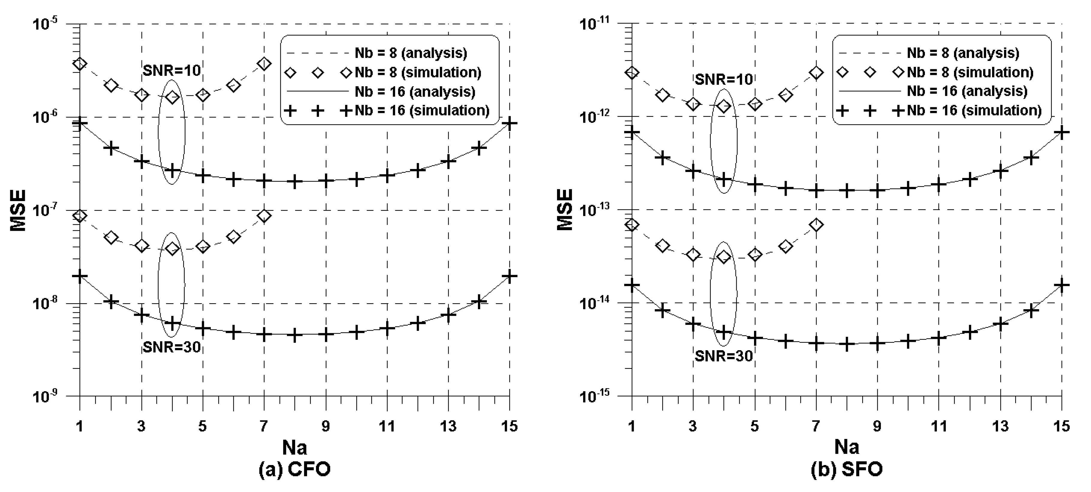
4.2. Pilot Subset Selection

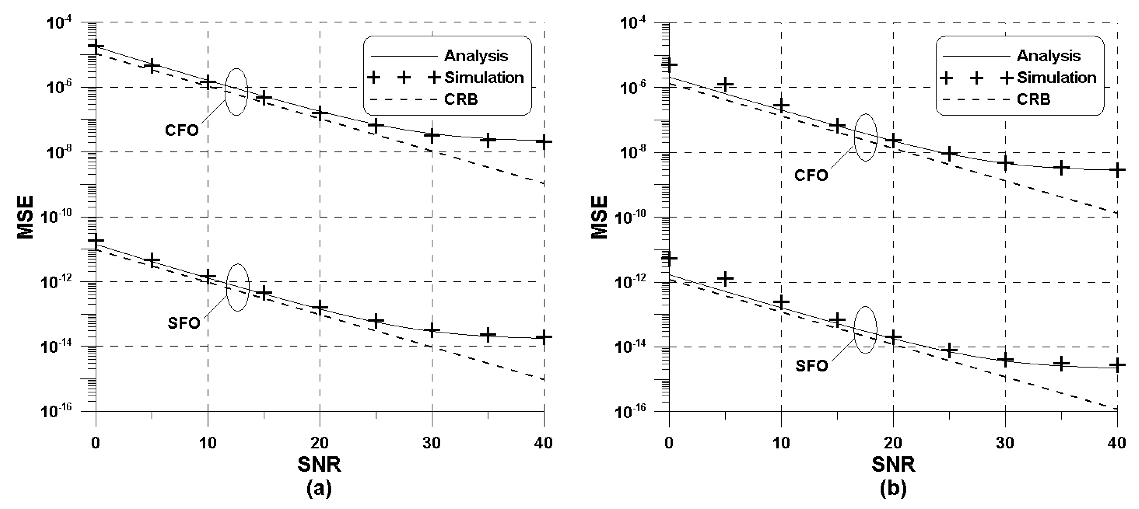
A close look at (35) and (36) reveals that the system parameters such as $N_b$, $N_g$ and N are predetermined, whereas non-zero valued $\epsilon$ and $\xi$ have to be estimated. Therefore, the first term in (35) is determined by variables $N_p$ and $L_p$, whereas the first term in (36) depends on variables $M_p$ and $L_p$. By using non-uniformly- and non-symmetrically-distributed CPs, the first two terms are left as non-zero constants, even as SNR grows, which makes the CFO and SFO estimates tightly related to one another. One possible way to separate these two estimation tasks is to group the CP subcarriers.

Therefore, the quantities $L_p$, $N_p$ and $M_p$ are important design parameters that must be selected appropriately. In order to minimize (35) and (36), one CP subset is chosen to enable $L_p$ to be minimized, as well as to enforce $N_p$ and $M_p$ to be maximized. To achieve this goal, a subset ${\mathcal{S}}_{\widehat{p}}$ is selected to meet the following criteria:

$$\begin{array}{c}\hfill \widehat{p}=\underset{1\le p\le N_c}{\arg \min }\left\{\frac{L_p^2}{N_p^2}\right\}\end{array}$$

(37)

and:

$$\begin{array}{c}\hfill \widehat{p}=\underset{1\le p\le N_c}{\arg \min }\left\{\frac{L_p^2}{M_p^2}\right\}\end{array}$$

(38)

where $N_c$ is the sum of the number of combinations choosing m subcarriers from $N_f$ subcarriers given by $N_c={\sum }_{m=1}^{N_f}{}_{N_f}{C}_m$.

As a consequence, the proposed LLSE scheme is in the same form as (32) and (33), replacing the subset index p with $\widehat{p}$ and putting $L_{\widehat{p}}=0$ thanks to the use of the optimal subset selected from (37) and (38). Assuming the channel is constant over $N_b$ OFDM symbols, the weighted version of the proposed LSE can be obtained similarly to (18) and (19):

$$\begin{array}{cc}\hfill \widehat{\epsilon }& =\frac{1}{\pi \beta N_b{\sum }_{k\in {\mathcal{S}}_{\widehat{p}}}{\left|{\tilde{H}}_l(k)\right|}^2}\sum _{k\in {\mathcal{S}}_{\widehat{p}}}{\left|{\tilde{H}}_l(k)\right|}^2\angle {\tilde{Y}}_l(k)\hfill \end{array}$$

(39)

and:

$$\begin{array}{cc}\hfill \widehat{\xi }& =\frac{1}{\pi \beta N_b{\sum }_{k\in {\mathcal{S}}_{\widehat{p}}}{k}^2{\left|{\tilde{H}}_l(k)\right|}^2}\sum _{k\in {\mathcal{S}}_{\widehat{p}}}k{\left|{\tilde{H}}_l(k)\right|}^2\angle {\tilde{Y}}_l(k).\hfill \end{array}$$

(40)

4.3. MSE Analysis

This section derives the MSE of (32) and (33) in the AWGN channel. For the purpose of notational convenience, (25) is rearranged into:

$$\begin{array}{cc}\hfill {\tilde{Y}}_l(k)& =E_{X}S(\phi (k))e^{j\pi \beta \phi (k)N_b}\left[1+\frac{\left\{{\mathcal{C}}_l(k)+{\mathcal{Z}}_l(k)\right\}{e}^{-j\pi \beta \phi (k)N_b}}{E_{X}S(\phi (k))}\right]\hfill \end{array}$$

(41)

where:

$$\begin{array}{cc}\hfill {\mathcal{C}}_l(k)& =\sum _{m=l}^{N_a+l-1}\sum _{q=N_a+l}^{N_b+l-1}{\tilde{C}}_{m,q}(k)\hfill \end{array}$$

(42)

and:

$$\begin{array}{cc}\hfill {\mathcal{Z}}_l(k)& =\sum _{m=l}^{N_a+l-1}\sum _{q=N_a+l}^{N_b+l-1}{\tilde{Z}}_{m,q}(k).\hfill \end{array}$$

(43)

Under the high SNR assumption [32] and CP boosting factor of 7/3, we make the useful approximation that:

$$\begin{array}{c}\hfill \widehat{\phi }(k)\approx \phi (k)+\frac{1}{\pi \beta N_b}\frac{{\tilde{\mathcal{C}}}_l^Q(k)+{\tilde{\mathcal{Z}}}_l^Q(k)}{E_{X}S(\phi (k))}\end{array}$$

(44)

where $X^Q$ denotes the imaginary component of a complex number X, ${\tilde{\mathcal{C}}}_l(k)={\mathcal{C}}_l(k)e^{-j\pi \beta \phi (k)N_b}$, and ${\tilde{\mathcal{Z}}}_l(k)={\mathcal{Z}}_l(k)e^{-j\pi \beta \phi (k)N_b}$. Notice that the statistics of ${\mathcal{C}}_l(k)$ and ${\mathcal{Z}}_l(k)$ are untouched after multiplying with $e^{-j\pi \beta \phi (k)N_b}$.

Since $L_{\widehat{p}}=0$ from the use of the optimal subset, substituting (44) into (29) and (30) produces the estimation error of the CFO and SFO estimator:

$$\begin{array}{cc}\hfill \widehat{\epsilon }-\epsilon & =\frac{1}{\pi \beta N_b{N}_{\widehat{p}}}\sum _{k\in {\mathcal{S}}_{\widehat{p}}}\frac{{\tilde{\mathcal{C}}}_l^Q(k)+{\tilde{\mathcal{Z}}}_l^Q(k)}{E_{X}S(\phi (k))}\hfill \end{array}$$

(45)

and:

$$\begin{array}{cc}\hfill \widehat{\xi }-\xi & =\frac{1}{\pi \beta N_b{M}_{\widehat{p}}}\sum _{k\in {\mathcal{S}}_{\widehat{p}}}k\frac{{\tilde{\mathcal{C}}}_l^Q(k)+{\tilde{\mathcal{Z}}}_l^Q(k)}{E_{X}S(\phi (k))}.\hfill \end{array}$$

(46)

After some straightforward manipulations, it turns out to be:

$$\begin{array}{cc}\hfill E\left\{{\left|\widehat{\epsilon }-\epsilon \right|}^2\right\}& ={\left(\frac{1}{\pi \beta N_b{N}_{\widehat{p}}{E}_X}\right)}^2\sum _{k\in {\mathcal{S}}_{\widehat{p}}}\frac{E\left\{{\left|{\tilde{\mathcal{C}}}_l^Q(k)\right|}^2\right\}+E\left\{{\left|{\tilde{\mathcal{Z}}}_l^Q(k)\right|}^2\right\}}{S{(\phi (k))}^2}\hfill \end{array}$$

(47)

and:

$$\begin{array}{cc}\hfill E\left\{{\left|\widehat{\xi }-\xi \right|}^2\right\}& ={\left(\frac{1}{\pi \beta N_b{M}_{\widehat{p}}{E}_X}\right)}^2\sum _{k\in {\mathcal{S}}_{\widehat{p}}}\frac{k^{2}E\left\{{\left|{\tilde{\mathcal{C}}}_l^Q(k)\right|}^2\right\}+k^{2}E\left\{{\left|{\tilde{\mathcal{Z}}}_l^Q(k)\right|}^2\right\}}{S{(\phi (k))}^2}.\hfill \end{array}$$

(48)

From (22) and (23), we obtain their variances ${\sigma }_{\tilde{C}}^2=E_X{\sigma }_C^2+{\sigma }_C^2{\sigma }_Z^2+{\sigma }_C^4/2$ and ${\sigma }_{\tilde{X}}^2=E_X{\sigma }_Z^2+{\sigma }_Z^4/2$, respectively. Bearing in mind that $E\left\{{\tilde{\mathcal{C}}}_l^Q(k)\right\}=E\left\{{\tilde{\mathcal{Z}}}_l^Q(k)\right\}=0$, the variances of ${\tilde{\mathcal{C}}}_l^Q(k)$ and ${\tilde{\mathcal{Z}}}_l^Q(k)$ are computed by:

$$\begin{array}{cc}\hfill E\left\{{\left|{\tilde{\mathcal{C}}}_l^Q(k)\right|}^2\right\}& =N_b(N_b-N_a)N_a(E_X{\sigma }_C^2+{\sigma }_C^2{\sigma }_Z^2)/2+(N_b-N_a)N_a{\sigma }_C^4/2\hfill \end{array}$$

(49)

and:

$$\begin{array}{cc}\hfill E\left\{{\left|{\tilde{\mathcal{Z}}}_l^Q(k)\right|}^2\right\}& =N_b(N_b-N_a)N_a{E}_X{\sigma }_Z^2/2+(N_b-N_a)N_a{\sigma }_Z^4/2\hfill \end{array}$$

(50)

which is put into (47) and (48). More importantly, $S(\phi (k))\approx (N_b-N_a)N_a$ for small enough values of $\epsilon$ and $\xi$. With those implications in mind, one gets:

$$\begin{array}{cc}\hfill E\left\{{\left|\widehat{\epsilon }-\epsilon \right|}^2\right\}& \approx \frac{1}{2{\pi }^2{\beta }^2{N}_b^2{N}_{\widehat{p}}(N_b-N_a)N_a}\left[\frac{N_b}{{\rho }_z}+\frac{1}{{\rho }_z^2}+\frac{1}{{\rho }_c}\left(N_b+\frac{N_b}{{\rho }_z}+\frac{1}{{\rho }_c}\right)\right]\hfill \end{array}$$

(51)

and:

$$\begin{array}{cc}\hfill E\left\{{\left|\widehat{\xi }-\xi \right|}^2\right\}& \approx \frac{1}{2{\pi }^2{\beta }^2{N}_b^2{M}_{\widehat{p}}(N_b-N_a)N_a}\left[\frac{N_b}{{\rho }_z}+\frac{1}{{\rho }_z^2}+\frac{1}{{\rho }_c}\left(N_b+\frac{N_b}{{\rho }_z}+\frac{1}{{\rho }_c}\right)\right]\hfill \end{array}$$

(52)

where ${\rho }_z=E_X/{\sigma }_Z^2$ is the SNR and ${\rho }_c=E_X/{\sigma }_C^2$ is the signal-to-ICI ratio. As a baseline for the performance of the estimators, we use the Cramer–Rao bound (CRB) for the estimates of $\epsilon$ and $\xi$ [29]:

$$\begin{array}{cc}\hfill CRB\left\{\epsilon \right\}& =\frac{3}{2{\pi }^2{\beta }^2{N}_{\widehat{p}}{N}_b(N_b^2-1){\rho }_z}·\frac{G(3)}{G(1)G(3)-G^2(2)}\hfill \end{array}$$

(53)

and:

$$\begin{array}{cc}\hfill CRB\left\{\xi \right\}& =\frac{3}{2{\pi }^2{\beta }^2{N}_{\widehat{p}}{N}_b(N_b^2-1){\rho }_z}·\frac{G(1)}{G(1)G(3)-G^2(2)}\hfill \end{array}$$

(54)

where $G(n)=(1/N_{\widehat{p}}){\sum }_{k\in {\mathcal{S}}_{\widehat{p}}}{k}^{n-1}$ for $n=1,2,3$.

It is obvious from (51) and (52) that the choice of some design parameters such as $M_{\widehat{p}}$, $N_{\widehat{p}}$, $N_b$ and $N_a$ has a significant impact on LLSE performance. Once the number of the OFDM block $N_b$ is chosen to be used for synchronization, the variables $N_{\widehat{p}}$ and $M_{\widehat{p}}$ are optimized by means of the pilot subset selection. Since these parameters are a priori known, which are treated as constants, the block size $N_a$ should be determined. The portion that relies on block size $N_a$ is obtained in (51) and (52), as follows:

$$\begin{array}{c}\hfill f(N_a)=\frac{1}{(N_b-N_a)N_a}.\end{array}$$

(55)

To find an optimal $N_a$ that minimizes the MSE of the proposed joint estimator, differentiation of (55) over $N_a$ is set to be zero, yielding:

$$\begin{array}{c}\hfill \frac{N_b-2N_a}{{(N_b-N_a)}^2{N}_a^2}=0\end{array}$$

(56)

where $0<N_a<N_b$. Therefore, (56) says that a unique solution is $N_a=N_b/2$

4.4. Computational Complexity

The complexity of the frequency-offset estimation methods is discussed in terms of the number of real floating point operations (flops). For a fair comparison, a complex multiplication is counted as six real flops, whereas a complex addition as two real flops [33]. We consider the situation where the channel estimation used to obtain ${\tilde{H}}_l(k)$ has been already performed at the receiver. The total number of real flops is calculated by $N_f(8N_b-7)-1$ for the conventional Scheme A, $N_f(6N_b^2-3N_b+13)+9$ for the conventional Scheme B and $8N_f{N}_b-2$ for the conventional Scheme C. On the other hand, the proposed LLSE scheme demands $N_{\widehat{p}}(2N_b+5)-1$ real flops, whereas $N_{\widehat{p}}(2N_b+12)-2$ flops are needed in the proposed WLSE scheme. If $N_f=N_{\widehat{p}}$ and $N_b>2$, it is evident that the complexity of the proposed LLSE method is always less than that of the conventional LLSE method, which is still true for the WLSE scenarios. A detailed computational complexity analysis is presented in Appendix A.

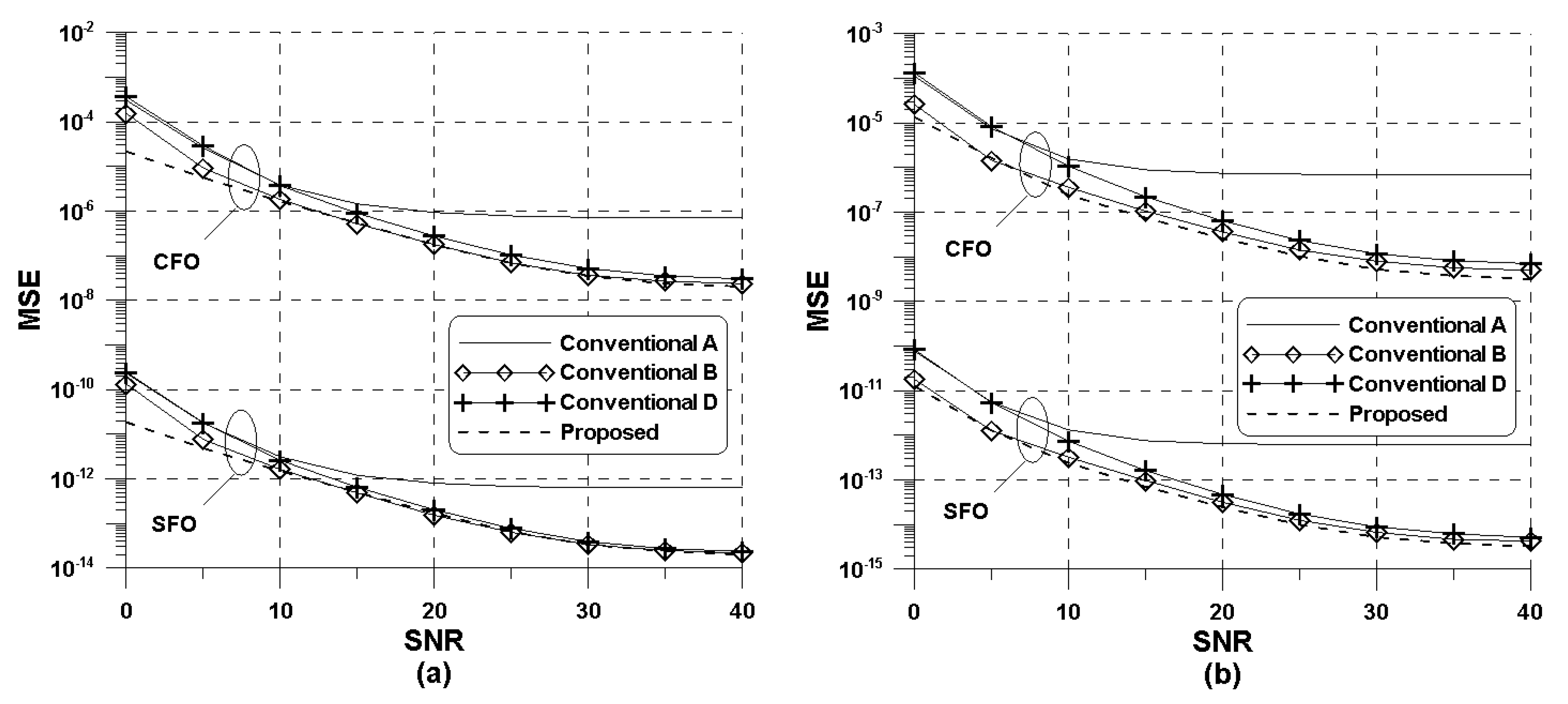
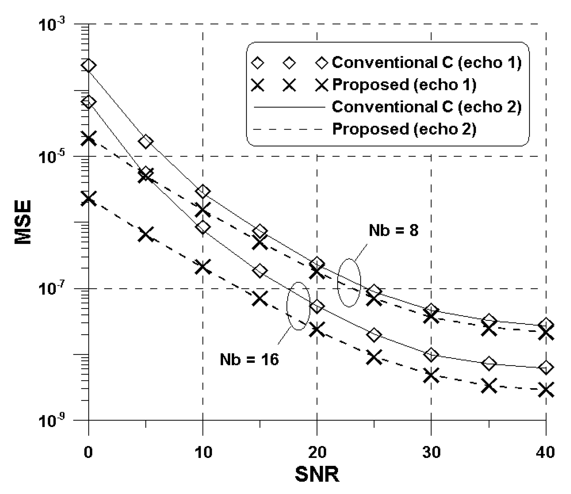
5. Simulation Results

In this section, the performance of the frequency-offset estimation schemes is assessed in accordance with the DVB-C2 standard using MATLAB software. Table 1 and Table 2 summarize the simulation parameters and channel profiles used in our experiments, respectively. The DVB-C2 OFDM system has $N=4096$, $N_g=64$ and $N_f=30$ subcarriers. The bandwidth of 8 MHz, the sampling time of $T_s=7/64$ $\mathsf{\mu }$s and 16 QAM are considered [10]. We simulate under AWGN and two echo channels specified in [11], which are based on the HFCchannel model. The CIR of echo channels can be described as:

$$\begin{array}{c}\hfill h(t)=1+\overline{\gamma }\sum _{i=1}^{N_e}{\gamma }_i{e}^{-j{\theta }_i}\delta (t-{\tau }_i)\end{array}$$

(57)

where $\overline{\gamma }={({\sum }_{i=1}^{N_e}{\gamma }_i^2)}^{-1/2}$, $N_e$ is the number of echoes, the path gain ${\gamma }_i$, the path delay ${\tau }_i$ and the path phase ${\theta }_i$, which are given in Table 2. Since $N_g=64$ is used, an echo delay of up to 7 $\mathsf{\mu }$s can be tolerated. For CFO and SFO, $\epsilon =0.02$ and $\xi =20$ ppm. The performance and complexity of the proposed WLSE method and the conventional Methods B and C are evaluated based on known CFR, while other schemes perform without relying on known CFR.

Table 1. System parameters. GI, guard interval; CP, continual pilot.

Parameters	Values
Bandwidth (Hz)	8 M
FFT size N	4096
Sampling time $T_s$ ($\mathsf{\mu }$s)	7/64
Subcarrier spacing $1/N{T}_s$ (Hz)	2232
Number of used subcarriers $N_z$	3408
Number of GI samples $N_g$	64
Number of CPs $N_f$	30
Subcarrier modulation	16 QAM

Table 2. Channel profiles.

i		Echo Channel 1				Echo Channel 2
	Power ${\mathit{\gamma }}_{\mathit{i}}$ (dB)	Delay ${\mathit{\tau }}_{\mathit{i}}$ (ns)	Phase ${\mathit{\theta }}_{\mathit{i}}$ (rad)		Power ${\mathit{\gamma }}_{\mathit{i}}$ (dB)	Delay ${\mathit{\tau }}_{\mathit{i}}$ (ns)	Phase ${\mathit{\theta }}_{\mathit{i}}$ (rad)
1	−11	38	0.95		−11	162	0.95
2	−14	181	1.67		−14	419	1.67
3	−17	427	0.26		−17	773	0.26
4	−23	809	1.20		−23	1191	1.20
5	−32	1633	1.12		−32	2067	1.12
6	−40	3708	0.81		−40	13,792	0.81

To estimate the CFO and SFO in a decoupled manner using (32) and (33), $L_p$ should be zero because of non-zero valued SFO and CFO in the first term of the RHS of (35) and (36), respectively. The goal of the pilot subset selection scheme is to make $L_p$ zero, as well as to maximize $N_p$ and $M_p$ at the same time. For this purpose, an optimal subset ${\mathcal{S}}_{\widehat{p}}$ is selected using the following procedure. For every possible number of combinations $N_c$, we search for a subset that satisfies (37), where the number of subsets can be one or more if $L_p=0$. In this case, the subset with the largest $N_p$ is chosen. If there is only one subset satisfying (37), this subset is the optimal one. Even after this process, there may be several subsets for the same $N_p$. Since the selected subsets all satisfy (38), if $L_p=0$, it is obvious that the subset giving the minimum MSE of the SFO estimator is the subset with the largest $M_p$. Through this exhaustive search, the optimal subset satisfying both (37) and (38) is found, and its value is $N_{\widehat{p}}=27$.

Figure 1 presents the comparison between the theoretical and simulation results of the proposed LLSE for various configurations in the AWGN. Since the size of the first block $N_a$ falls inside $0<N_a<N_b$, the range of the x-axis is $1\le N_a\le N_b-1$. It is evident that the analytical results are in perfect agreement with the simulated results in the AWGN channel. Hence, one can see that the optimal $N_a$ obtained from (56) exactly accords with the value simulated in Figure 1. It is worthwhile to notice that the performance is symmetric with respect to $N_a=N_b/2$. This is due to the fact that the representation of block-by-block correlation (20) in the symmetric position around $N_a=N_b/2$ is the same except for the conjugate locations because the sum of the sizes of the two blocks is $N_b$. From now on, the optimal value $N_a$ will be used in the proposed scheme.

Figure 1. Performance of the proposed linear LSE (LLSE) method versus $N_a$ in the AWGN channel: (a) carrier frequency offset (CFO) estimation; (b) sampling frequency offset (SFO) estimation.

Figure 2 depicts the comparison between the theoretical and simulation results of the proposed LLSE method versus SNR in the AWGN channel. The CRBs using (53) and (54) are also presented as a baseline. There is a small gap between the analysis and simulation results at low SNR because of the approximation used in (44). For a wide range of SNR values, however, the analysis and simulation results are very close to each other. We observe that the proposed scheme comes close to the CRB in low and medium SNR regions, whereas the CRB is not attainable even as the SNR increases because the ICI is no longer negligible.

Figure 2. Performance of the proposed LLSE method versus SNR in the AWGN channel: (a) $N_b=8$; (b) $N_b=16$.

Figure 3 and Figure 4 show the MSE of the frequency-offset estimation methods in Echo Channels 1 and 2, having a maximum delay of 3.7 $\mathsf{\mu }$ and 13.8 $\mathsf{\mu }$, respectively. In the example, the conventional Scheme D corresponds to (10) and (11) when ${\mathcal{S}}_{\widehat{p}}$ is used instead of ${\mathcal{S}}_f$, which is a simple extension of the work in [25] and needs $N_{\widehat{p}}(8N_b-7)-1$ real flops. As reported in the literature, non-negligible ICI leads to an error floor in the frequency-offset estimation schemes when the SNR is high. The conventional Scheme A suffers from severe irreducible error floor owing to non-symmetrically-distributed CPs, whereas the conventional Scheme D benefits from the selected pilot subset, so that its performance approaches that of the proposed scheme for higher SNR values. In Echo Channel 1, the MSE of the proposed LLSE method is slightly better than that of the conventional Method B, particularly at low SNR values. This phenomenon becomes insignificant as $N_b$ increases. The amounts of phase rotation of the conventional Schemes A, B and C caused by frequency offsets are all $2\pi \beta$, whereas that of the proposed scheme is $\pi \beta N_b$. If the number of observed OFDM symbols is $N_b>2$, the amount of phase rotation of the proposed scheme is greater than that of the conventional schemes, which makes the proposed estimator less sensitive to the noise, especially for a low SNR regime. With the increase of the frequency selectivity in Echo Channel 2, the performance gain of the conventional Scheme B over the proposed LLSE scheme is observed for $SNR>10$ dB. Such a gain of the conventional Scheme B is paid for by far higher computational processing. When $N_b=8$, the total number of real flops used in the proposed LLSE using $N_{\widehat{p}}=27$ is saved by 66.9%, 94.9% and 63.2% compared to that of the existing Methods A, B and D, respectively.

Figure 3. Performance of the frequency-offset estimation methods in Echo Channel 1: (a) $N_b=8$; (b) $N_b=16$.

Figure 4. Performance of the frequency-offset estimation methods in Echo Channel 2: (a) $N_b=8$; (b) $N_b=16$.

Figure 5 depicts the performance of the existing and proposed WLSE method in Echo Channel 1 and Echo Channel 2, using the same simulation parameters as in Figure 3 and Figure 4. In this example, the conventional WLSE scheme (18) using ${\mathcal{S}}_{\widehat{p}}$ instead of ${\mathcal{S}}_f$ is included, whereas the proposed scheme corresponds to (39). As predicted, we observe that the proposed WLSE approach still outperforms the conventional WLSE scheme with the aid of block-by-block estimation. It is clear that there is no significant performance difference between two echo channels in contrast to other methods, as illustrated in Figure 3 and Figure 4. This phenomenon is attributed to the fact that the WLS approach is able to mitigate the effect of frequency selectivity on the different subcarriers. Regarding the complexity of both methods, the flops of the proposed WLSE scheme when $N_b=8$ and 16 are reduced by 56.3% and 65.7% when compared to that of the existing WLSE method, respectively. Note that increasing $N_b$ eases the computational requirement of the proposed scheme at the sacrifice of estimation range.

Figure 5. Performance of the conventional and proposed WLSE methods in Echo Channels 1 and 2.

6. Conclusions

To make full use of the attractive benefits of OFDM in the DVB-C2 system, it is very important to keep the frequency alignment between the transmitter and the receiver. In this study, a reduced-complexity and robust CFO and SFO estimation method was suggested in the DVB-C2 OFDM system, which is based on a block-by-block estimation. The block-by-block estimation was used to make the LSE be complexity effective and noise robust. The optimization of the LSE scheme played an important role in minimizing a bias from non-symmetrically located CPs. Since the amount of phase rotation of the proposed estimation scheme caused by frequency offsets increases in proportion to the number of observed symbols, the proposed method could provide robustness against noise. It has been demonstrated by the presented results that the proposed block-by-block estimation method is proven to be computationally efficient, offering an improved estimation performance, when compared with the conventional estimation methods. Therefore, the proposed frequency-offset estimation scheme can be used to maximize the benefits of OFDM in digital cable communication systems.

Appendix A.1. Conventional Scheme A

Recall that the conventional scheme A is based on three operations: the averaged correlation $Y_l(k)$ in (6), the CFO estimation in (10) and the SFO estimation in (11). For each CP subcarrier, it follows from (6) that $Y_l(k)$ requires $N_b-1$ complex multiplications and $N_b-2$ complex additions, which is converted to $8N_b-10$ real flops. To estimate the CFO $\widehat{\epsilon }$ in (10), the summation over $k\in {\mathcal{S}}_f$ requires $N_f-1$ real additions, and the calculation of $\angle Y_l(k)$ consumes $N_f(8N_b-10)$ real flops for $N_f$ subcarriers. Thus, (10) requires $N_f(8N_b-9)$ real flops. For the estimation of SFO $\widehat{\xi }$ in (11), the summation over $k\in {\mathcal{S}}_f$, denoted by ${\sum }_{k\in {\mathcal{S}}_f}k\angle Y_l(k)$, demands $N_f$ real multiplications and $N_f-1$ real additions. With those calculations in mind, we conclude that the conventional Scheme A uses $N_f(8N_b-7)-1$ real flops.

Appendix A.2. Conventional Scheme B

Bear in mind that the conventional scheme B is comprised of four operations: the g-lag correlation ${\overline{Y}}_g(k)$ in (12), the estimation of total frequency offsets $\widehat{\phi }(k)$ in (13), the CFO estimation in (14) and the SFO estimation in (15). In (12), it can be seen that using ${\overline{Y}}_g(k)$ requires $N_f(3N_b^2/8-N_b/4)$ complex multiplications and $N_f(3N_b^2/8-3N_b/4)$ complex additions. For (13), ${\overline{Y}}_{g-1}(k)$ is also calculated, which requires $N_f(3N_b^2/8-3N_b/4)$ complex multiplications and $N_f(3N_b^2/8-5N_b/4+1)$ complex additions. To estimate $\widehat{\phi }(k)$ in (13), it follows that computing ${\sum }_{g=1}^{N_b/2}w(g)\angle {\overline{Y}}_g(k){\overline{Y}}_{g-1}^{*}(k)$ requires $N_f(N_b/2)$ complex multiplications, $N_f(N_b/2)$ real multiplications and $N_f(N_b/2-1)$ real additions. For $W(n)$’s and $Q(n)$’s, $W(n)$’s ($n=1,2,3$) require $4N_f$ real multiplications and $4N_f-3$ real additions, whereas the calculation of $Q(n)$’s ($n=1,2$) needs $2N_f$ real multiplications and $2N_f-2$ real additions. The calculation of (14) and (15) demands 10 real multiplications and four real additions. As a consequence, the conventional Scheme B requires the number of real flops given by $N_f(6N_b^2-3N_b+13)+9$.

Appendix A.3. Conventional Scheme C

In the case of the conventional scheme C, its complexity is based on the computations of (6), (18) and (19). The number of operations in (6) is the same as that in the conventional Scheme A. From (18), ${\sum }_{k\in {\mathcal{S}}_f}{\left|{\tilde{H}}_l(k)\right|}^2\angle Y_l(k)$ requires $3N_f$ real multiplications and $2N_f-1$ real additions, whereas $N_f-1$ real additions are needed for calculating ${\sum }_{k\in {\mathcal{S}}_f}{\left|{\tilde{H}}_l(k)\right|}^2$. For each CP subcarrier, $\angle Y_l(k)$ is performed, and the summation over $k\in {\mathcal{S}}_f$ requires $N_f(8N_b-10)$ real flops. Then, the number of operations in (18) is $N_f(8N_b-4)-1$ real flops. Estimating SFO $\widehat{\xi }$ in (19), it follows that calculating the quantity ${\sum }_{k\in {\mathcal{S}}_f}k{\left|{\tilde{H}}_l(k)\right|}^2\angle Y_l(k)$ needs $N_f$ real multiplications and $N_f-1$ real additions because some intermediate results in (18) are already available, whereas ${\sum }_{k\in {\mathcal{S}}_f}{k}^2{\left|{\tilde{H}}_l(k)\right|}^2$ requires $N_f$ real multiplications and $N_f-1$ real additions. Thus, it is concluded that $8N_f{N}_b-2$ real flops are needed in the conventional Scheme C.

Appendix A.4. Proposed Scheme

The computational burden of the proposed LLSE method mainly depends on the operations of the block-by-block correlation in (20), the CFO estimation in (29) and the SFO estimation in (30). For each CP subcarrier, it follows from (20) that ${\tilde{Y}}_l(k)$ requires one complex multiplication and $N_b-2$ complex additions, which is converted to $2(N_b+1)$ real flops. For the estimation of CFO $\widehat{\epsilon }$ in (29), it is performed for each CP subcarrier, and the summation over $k\in {\mathcal{S}}_{\widehat{p}}$ requires $N_{\widehat{p}}-1$ real additions. For $N_{\widehat{p}}$ subcarriers, $\angle {\tilde{Y}}_l(k)$ needs $N_{\widehat{p}}(2N_b+2)$ real flops. Eventually, $N_{\widehat{p}}(2N_b+3)$ real flops are used in (29). To estimate the SFO $\widehat{\xi }$ in (30), the summation over $k\in {\mathcal{S}}_{\widehat{p}}$, denoted by ${\sum }_{k\in {\mathcal{S}}_{\widehat{p}}}k\angle {\tilde{Y}}_l(k)$, requires $N_{\widehat{p}}$ real multiplications and $N_{\widehat{p}}-1$ real additions. With those calculations in mind, it can be seen that the proposed LLSE scheme requires $N_{\widehat{p}}(2N_b+5)-1$ real flops.

In the case of the proposed WLSE method, the computational operations of (39) and (40) are exactly the same as those of (18) and (19), except for the computation of (20). Since the presence of $|{\tilde{H}}_l{(k)|}^2$ additionally consumes $4N_f$ real multiplications and $3N_f-1$ real additions in the WLSE compared to the LLSE, one can easily find that $N_{\widehat{p}}(2N_b+12)-2$ real flops are demanded in the proposed WLSE scheme.

References

1. ETSI EN 302 755 V.1.4.1. Digital Video Broadcasting (DVB); Frame Structure Channel Coding and Modulation for a Second Generation Digital Terrestrial Television Broadcasting System (DVB-T2); ETSI: Sophia Antipolis, France, 2015. [Google Scholar]
2. 3GPP TS36.211. Evolved Universal Terrestrial Radio Access (EUTRA); Physical Channels and Modulation; Release 12; 3GPP: Phoenix, AZ, USA, 2015. [Google Scholar]
3. IEEE Std 802.11a. Wireless LAN Medium Access Control (MAC) and Physical Layer (PHY) Specification: High-Speed Physical Layer in the 5GHz Band; IEEE: Piscataway, NJ, USA, 1999. [Google Scholar]
4. Cvijetic, N. OFDM for next-generation optical access networks. J. Lightw. Technol. 2012, 30, 384–398. [Google Scholar] [CrossRef]
5. Shoresh, T.; Katanov, N.; Malka, D. 1 × 4 MMI visible light wavelength demultiplexer based on GaN slot waveguide structures. J. Photon. Nanostruct. Fundam. Appl. 2018, 30, 45–49. [Google Scholar] [CrossRef]
6. Malka, D.; Katz, G. An eight-channel C-band demuxbased on multicore photonic crystal fiber. Nanomaterials 2018, 8, 845. [Google Scholar] [CrossRef] [PubMed]
7. Dadabayev, R.; Shabairoub, N.; Zalevsky, Z.; Malka, D. A visible light RGB wavelength demultiplexer based on silicon-nitride multicore PCF. Opt. Laser Technol. 2019, 111, 411–416. [Google Scholar] [CrossRef]
8. HomePlug Powerline Alliance, Inc. Homeplug Green PHY Specification Release Version 1.1.1; HomePlug Alliance: Portland, OR, USA, 2013. [Google Scholar]
9. IEEE 1901-2010. IEEE Standard for Broadband over Power Line Networks: Medium Access Control and Physical Layer Specifications; IEEE: New York, NY, USA, 2010. [Google Scholar]
10. ETSI EN 302 769 V1.3.1. Digital Video Broadcasting (DVB). Frame Structure Channel Coding and Modulation for a Second Generation Digital Transmission System for Cable Systems (DVB-C2); ETSI: Sophia Antipolis, France, 2015. [Google Scholar]
11. DVB Document A147, Digital Video Broadcasting (DVB). Implementation Guidelines for a Second Generation Digital Cable Transmission System (DVB-C2); ETSI: Sophia Antipolis, France, 2015. [Google Scholar]
12. Jaeger, D.; Schaaf, C. DVB-C2: High Performance Data Transmission on Cable:-Technology, Implementation, Networks; Shaker Verlag GmbH: Herzogenrath/Maastricht, Germany, 2010. [Google Scholar]
13. El-Hajjar, M.; Hanzo, L. A survey of digital television broadcast transmission techniques. IEEE Commun. Surv. Tutor. 2013, 15, 1924–1941. [Google Scholar] [CrossRef]
14. Lee, J.H.; Choi, D.J.; Hur, N.H.; Kim, W.W. Performance analysis of a proposed pre-FEC structure for a DVB-C2 receiver. IEEE Trans. Broadcast. 2013, 59, 638–647. [Google Scholar] [CrossRef]
15. Lee, J.H.; Choi, D.J.; Hur, N.H.; Kim, W.W. The performance of frequency offset estimation in DVB-C2 receiver. In Proceedings of the 2013 International Conference on Advanced Communication Technology (ICACT), PyeongChang, Korea, 27–30 January 2013; pp. 1106–1110. [Google Scholar]
16. Speth, M.; Fechtel, S.A.; Fock, G.; Meyr, H. Optimum receiver design for wireless broad-band systems using OFDM-Part I. IEEE Trans. Commun. 1999, 47, 1668–1677. [Google Scholar] [CrossRef]
17. Oberli, C. ML-based tracking algorithms for MIMO-OFDM. IEEE Trans. Wirel. Commun. 2007, 6, 2630–2639. [Google Scholar] [CrossRef]
18. Yuan, J.; Torlak, M. Joint CFO and SFO estimator for OFDM receiver using common reference frequency. IEEE Trans. Broadcast. 2016, 62, 141–149. [Google Scholar] [CrossRef]
19. Kim, Y.H.; Lee, J.H. Joint maximum likelihood estimation of carrier and sampling frequency offsets for OFDM systems. IEEE Trans. Broadcast. 2013, 57, 277–283. [Google Scholar]
20. Zhou, M.; Feng, Z.; Liu, Y.; Huang, X. An efficient algorithm and hardware architecture for maximum-likelihood based carrier frequency offset estimation in MIMO systems. IEEE Access 2018, 6, 50105–50116. [Google Scholar] [CrossRef]
21. Speth, M.; Fechtel, S.A.; Fock, G.; Meyr, H. Optimum receiver design for OFDM-based broadband transmission-Part II: A case study. IEEE Trans. Commun. 2001, 49, 571–578. [Google Scholar] [CrossRef]
22. Shi, K.; Serpedin, E.; Ciblat, P. Decision-directed fine synchronization in OFDM systems. IEEE Trans. Commun. 2005, 53, 408–412. [Google Scholar] [CrossRef]
23. Liu, S.; Chong, J.A. Study of joint tracking algorithms of carrier frequency offset and sampling clock offset for OFDM-based WLANs. In Proceedings of the 2002 International Conference on Communications, Circuits and Systems and West Sino Expositions, Chengdu, China, 29 June–1 July 2002; pp. 109–113. [Google Scholar]
24. Kwon, K.W.; Cho, Y.S. A simple joint estimation method of residual frequency offset and sampling frequency offset for DVB systems. IEICE Trans. Commun. 2008, E91-B, 1673–1676. [Google Scholar] [CrossRef]
25. Jung, Y.A.; Kim, J.Y.; You, Y.H. Complexity efficient least squares estimation of frequency offsets for DVB-C2 OFDM systems. IEEE Access 2018, 6, 35165–35170. [Google Scholar] [CrossRef]
26. Tsai, P.Y.; Kang, H.Y.; Chiueh, T.D. Joint weighted least-squares estimation of carrier-frequency offset and timing offset for OFDM systems over multipath fading channels. IEEE Trans. Veh. Technol. 2005, 1, 211–223. [Google Scholar] [CrossRef]
27. Chiang, P.; Lin, D.; Li, H.; Stuber, G.L. Joint estimation of carrier-frequency and sampling-frequency offsets for SC-FDE systems on multipath fading channels. IEEE Trans. Commun. 2008, 56, 1231–1235. [Google Scholar] [CrossRef]
28. Lin, Y.; Chen, S. A blind fine synchronization scheme for SC-FDE systems. IEEE Trans. Commun. 2014, 62, 293–301. [Google Scholar] [CrossRef]
29. Morelli, M.; Moretti, M. Fine carrier and sampling frequency synchronization in OFDM systems. IEEE Trans. Wirel. Commun. 2010, 4, 1514–1524. [Google Scholar] [CrossRef]
30. Murin, Y.; Dabora, R. Low complexity estimation of carrier and sampling frequency offsets in burst-mode OFDM systems. Wirel. Commun. Mob. Comput. 2016, 16, 1018–1034. [Google Scholar] [CrossRef]
31. Cheng, Q. Joint estimation of carrier and sampling frequency offsets using OFDM WLAN preamble. Wirel. Person. Commun. 2018, 98, 2121–2161. [Google Scholar] [CrossRef]
32. Fowler, M. Phase-based frequency estimation: A review. Digit. Signal Process. 2002, 4, 590–615. [Google Scholar] [CrossRef]
33. Golub, G.H.; Vanloan, C.F. Matrix Computations; The Johns Hopkins University Press: Baltimore, MA, USA, 1996. [Google Scholar]