Abstract
The definition of a Detour–Harary index is , where G is a simple and connected graph, and is equal to the length of the longest path between vertices u and v. In this paper, we obtained the maximum Detour–Harary index about unicyclic graphs, bicyclic graphs, and cacti, respectively.
1. Introduction
In recent years, chemical graph theory (CGT) has been fast-growing. It helps researchers to understand the structural properties of a molecular graph, for example, References [1,2,3].
A simple graph is an undirected graph without multiple edges and loops. Let G be a simple and connected graph, and and be the vertex set and edge set of G, respectively. For vertices of G, (or for short) is the distance between and , which equals to the length of the shortest path between and in G; (or for short) is the detour distance between and , which equals to the longest path of a shortest path between and in G.
is an induced subgraph of G, the vertex set is S, and the edge set is the set of edges of G and both ends in S. is the induced subgraph ; when , we write for short.
In 1947, Wiener introduced the first molecular topological index–Wiener index. The Wiener index has applications in many fields, such as chemistry, communication, and cryptology [4,5,6,7]. Moreover, the Wiener index was studied from a purely graph-theoretical point of view [8,9,10]. In Reference [11], Wiener gave the definition of the Wiener index:
The Harary index was independently introduced by Plavšić et al. [12] and by Ivanciuc et al. [13] in 1993. In References [12,13], they gave the definition of the Harary index:
In Reference [13], Ivanciuc gave the definition of the Detour index:
Lukovits [14] investigated the use of the Detour index in quantitative structure–activity relationship (QSAR) studies. Trinajstić and his collaborators [15] analyzed the use of the Detour index, and compared its application with Wiener index. They found that the Detour index in combination with the Wiener index is very efficient in the structure-boiling point modeling of acyclic and cyclic saturated hydrocarbons.
In this paper, we introduce a new graph invariant reciprocal to the Detour index, namely, the Detour–Harary index, as
Let G be a simple and connected graph, and . If , then G is a tree; if , then G is a unicyclic graph; if , then G is a bicyclic graph.
Suppose is the set of unicyclic (bicyclic, respectively) graphs set with n vertices. Any bicyclic graph G can be obtained from -graph or -graph by attaching trees to the vertices, where , and at most one of them is equal to 1. We denote be the kernel of G (Figure 1).
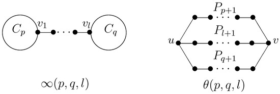
Figure 1.
∞-graph and -graph.
If each block of G is either a cycle or an edge, then we called graph G a cactus graph. Suppose be the set of all cacti with n-vertices and k cycles. Obviously, are trees, are unicyclic graphs, and are bicyclic graphs with exactly two cycles.
There are more results about cacti and bicyclic graphs [16,17,18,19,20,21,22,23,24,25]. More results about Harary index can be found in References [26,27,28,29,30,31,32,33,34], and more results about Detour index can be found in References [14,35,36,37,38,39].
Note that the Detour–Harary index is the same as Harary index for a tree graph; we study the Detour–Harary index of topological structures containing cycles. In this paper, we gave the maximum Detour–Harary index among , and , respectively.
2. Preliminaries
In this section, we introduce useful lemmas and graph transformations.
Lemma 1.
[40] Let G be a connected graph, x be a cut-vertex of G, and u and v be vertices occurring in different components that arise upon the deletion of vertex x. Then
2.1. Edge-Lifting Transformation
The edge-lifting transformation [41]. Let and be two graphs with and vertices. and , G is the graph obtained from and by adding an edge between and . is the graph obtained by identifying to and adding a pendent edge to . We called graph the edge-lifting transformation of graph G (see Figure 2).
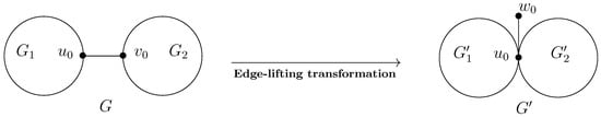
Figure 2.
Edge-lifting transformation.
Lemma 2.
Let graph be the edge-lifting transformation of graph G. Then .
Proof.
By the definition of and Lemma 1,
Obviously,
Then
□
2.2. Cycle-Edge Transformation
Suppose is a cactus as shown in Figure 3. is a cycle of G; is a cactus, and , ; , . is the graph obtained from G by deleting the edges from to , while adding the edges from to .
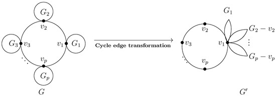
Figure 3.
Cycle-edge transformation.
We called graph the cycle-edge transformation of graph G (see Figure 3).
Lemma 3.
Suppose is a cactus, , and is the cycle-edge transformation of G (see Figure 3). Then, , and the equality holds if and only if .
Proof.
Let , . By the definition of and Lemma 1,
Obviously,
Then
The proof is completed. □
2.3. Cycle Transformation
Suppose is a cactus, as shown in Figure 4. is a cycle of G, and is a simple and connected graph, . is the graph obtained from G by deleting the edges from to , meanwhile, adding the edges from to .
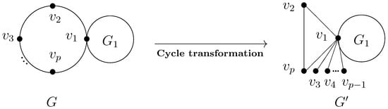
Figure 4.
Cycle transformation.
Lemma 4.
Suppose graph G is a simple and connected graph with , and is the cycle transformation of G(see Figure 4). Then, .
Proof.
Let , , . By the definition of ,
Obviously,
Then
□
3. Maximum Detour–Harary Index of Unicyclic Graphs
For any unicyclic graph , by repeating edge-lifting transformations, cycle-edge transformations, cycle transformations, or any combination of these on G, we get from G, where graph is defined in Figure 5.
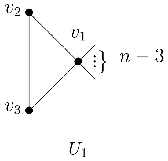
Figure 5.
Unicyclic graph .
Theorem 1.
Let be defined as Figure 5. Then, is the unique graph that attains the maximum Detour–Harary index among all graphs in , and
Proof.
By Lemmas 2–4, is the unique graph which attains the maximum Detour–Harary index of all graphs in . We then calculate the value .
Let It can be checked directly that
Then
The proof is completed. □
4. Maximum Detour–Harary Index of Bicyclic Graphs
For any bicyclic graph with exactly two cycles, by repeating edge-lifting transformations, cycle-edge transformations, cycle transformations, or any combination of these on G, we get from G, where graph is defined in Figure 6.
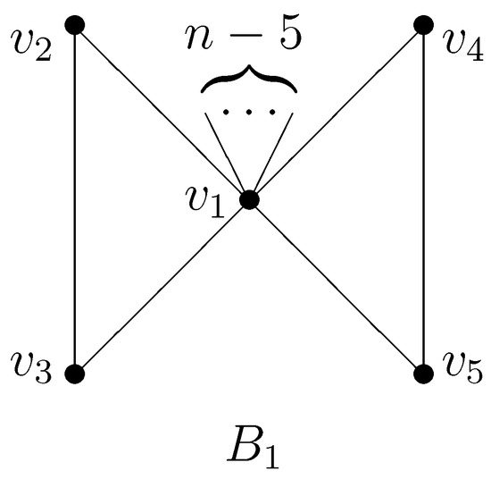
Figure 6.
Bicyclic graph .
For any bicyclic graph with n vertices, by repeating edge-lifting transformations on G, we get from G, where graph is defined in Figure 7.
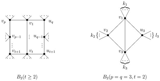
Figure 7.
Bicyclic graph ().
Theorem 2.
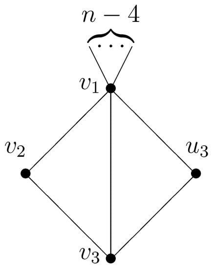
Figure 8.
Bicyclic graph ().
Proof.
Case 1. . Obviously,
Let , and and , and and for .
Easily,
Then,
the equality holds if and only if .
On the other hand , where , then
the equality holds if or or or .
By (1)–(3) and , we have .
Case 3. and .
It can be checked directly that
are bicyclic graphs and . Since then and , we have
The proof is completed. □
Proof.
Let , by Lemmas 2–4, we have , and the equality holds if and only if
For any bicyclic graph with , by Lemmas 2–4 and Theorem 2, we have , and the equality holds if and only if Thus, .
It can be checked directly that
Therefore
The proof is completed. □
5. Maximum Detour–Harary Index of Cacti
For any cactus graph , by repeating edge-lifting transformations, cycle-edge transformations, cycle transformations, or any combination of these on G, we get from G, where graph is defined in Figure 9.
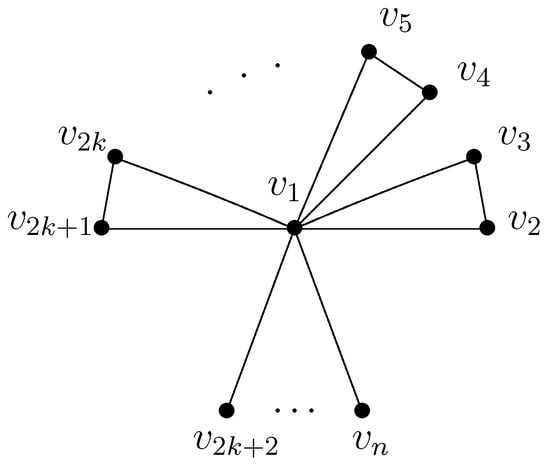
Figure 9.
Cactus graph .
Theorem 4.
Let be defined as Figure 9. Then, is the unique cactus graph in that attains the maximum Detour–Harary index, and
Proof.
By Lemmas 2–4, is the unique graph that attains the maximum Detour–Harary index of all graphs in .
Let , and it can be checked directly that
Then,
The proof is completed. □
Author Contributions
Conceptualization, W.F. and W.-H.L.; methodology, F.-Y.C.; Z.-J.X. and J.-B.L.; writing—original draft preparation, W.F. and Z.-M.H; writing—review and editing, W.-H.L.
Funding
This research was funded by NSFC Grant (No.11601001, No.11601002, No.11601006).
Conflicts of Interest
The authors declare no conflict of interest.
References
- Imran, M.; Ali, M.A.; Ahmad, S.; Siddiqui, M.K.; Baig, A.Q. Topological sharacterization of the symmetrical structure of bismuth tri-iodide. Symmetry 2018, 10, 201. [Google Scholar] [CrossRef]
- Liu, J.; Siddiqui, M.K.; Zahid, M.A.; Naeem, M.; Baig, A.Q. Topological Properties of Crystallographic Structure of Molecules. Symmetry 2018, 10, 265. [Google Scholar] [CrossRef]
- Shao, Z.; Siddiqui, M.K.; Muhammad, M.H. Computing zagreb indices and zagreb polynomials for symmetrical nanotubes. Symmetry 2018, 10, 244. [Google Scholar] [CrossRef]
- Dobrynin, A.; Entringer, R.; Gutman, I. Wiener Index of Trees: Theory and Applications. Acta Appl. Math. 2001, 66, 211–249. [Google Scholar] [CrossRef]
- Alizadeh, Y.; Andova, V.; Zar, S.K.; Skrekovski, R.V. Wiener dimension: Fundamental properties and (5,0)-nanotubical fullerenes. MATCH Commun. Math. Comput. Chem. 2014, 72, 279–294. [Google Scholar]
- Needham, D.E.; Wei, I.C.; Seybold, P.G. Molecular modeling of the physical properties of alkanes. J. Am. Chem. Soc. 1988, 110, 4186–4194. [Google Scholar] [CrossRef]
- Vijayabarathi, A.; Anjaneyulu, G.S.G.N. Wiener index of a graph and chemical applications. Int. J. ChemTech Res. 2013, 5, 1847–1853. [Google Scholar]
- Gutman, I.; Cruz, R.; Rada, J. Wiener index of Eulerian graphs. Discret. Appl. Math. 2014, 162, 247–250. [Google Scholar] [CrossRef]
- Lin, H. Extremal Wiener index of trees with given number of vertices of even degree. MATCH Commun. Math. Comput. Chem. 2014, 72, 311–320. [Google Scholar]
- Lin, H. Note on the maximum Wiener index of trees with given number of vertices of maximum degree. MATCH Commun. Math. Comput. Chem. 2014, 72, 783–790. [Google Scholar]
- Wiener, H. Structural determination of paraffin boiling points. Am. Chem. Soc. 1947, 69, 17–20. [Google Scholar] [CrossRef]
- Plavšić, D.; Nikolić, S.; Trinajstić, N.; Mihalić, Z. On the Harary index for the characterization of chemical graphs. J. Math. Chem. 1993, 12, 235–250. [Google Scholar] [CrossRef]
- Ivanciuc, O.; Balaban, T.S.; Balaban, A.T. Reciprocal distance matrix, related local vertex invariants and topological indices. J. Math. Chem. 1993, 12, 309–318. [Google Scholar] [CrossRef]
- Lukovits, I. The Detour index. Croat. Chem. Acta 1996, 69, 873–882. [Google Scholar]
- Trinajstić, N.; Nikolić, S.; Lučić, B.; Amić, D.; Mihalić, Z. The Detour matrix in chemistry. J. Chem. Inf. Comput. Sci. 1997, 37, 631–638. [Google Scholar] [CrossRef]
- Chen, S. Cacti with the smallest, second smallest, and third smallest Gutman index. J. Comb. Optim. 2016, 31, 327–332. [Google Scholar] [CrossRef]
- Chen, Z.; Dehmer, M.; Shi, Y.; Yang, H. Sharp upper bounds for the Balaban index of bicyclic graphs. MATCH Commun. Math. Comput. Chem. 2016, 75, 105–128. [Google Scholar]
- Fang, W.; Gao, Y.; Shao, Y.; Gao, W.; Jing, G.; Li, Z. Maximum Balaban index and sum-Balaban index of bicyclic graphs. MATCH Commun. Math. Comput. Chem. 2016, 75, 129–156. [Google Scholar]
- Fang, W.; Wang, Y.; Liu, J.-B.; Jing, G. Maximum Resistance-Harary index of cacti. Discret. Appl. Math. 2018. [Google Scholar] [CrossRef]
- Gutman, I.; Li, S.; Wei, W. Cacti with n-vertices and t-cycles having extremal Wiener index. Discret. Appl. Math. 2017, 232, 189–200. [Google Scholar] [CrossRef]
- Ji, S.; Li, X.; Shi, Y. Extremal matching energy of bicyclic graphs. MATCH Commun. Math. Comput. Chem. 2013, 70, 697–706. [Google Scholar]
- Liu, J.; Pan, X.; Yu, L.; Li, D. Complete characterization of bicyclic graphs with minimal Kirchhoff index. Discret. Appl. Math. 2016, 200, 95–107. [Google Scholar] [CrossRef]
- Wang, H.; Hua, H.; Wang, D. Cacti with minimum, second-minimum, and third-minimum Kirchhoff indices. Math. Commun. 2010, 15, 347–358. [Google Scholar]
- Wang, L.; Fan, Y.; Wang, Y. Maximum Estrada index of bicyclic graphs. Discret. Appl. Math. 2015, 180, 194–199. [Google Scholar] [CrossRef]
- Lu, Y.; Wang, L.; Xiao, P. Complex Unit Gain Bicyclic Graphs with Rank 2,3 or 4. Linear Algebra Appl. 2017, 523, 169–186. [Google Scholar] [CrossRef]
- Furtula, B.; Gutman, I.; Katanić, V. Three-center Harary index and its applications. Iran. J. Math. Chem. 2016, 7, 61–68. [Google Scholar]
- Feng, L.; Lan, Y.; Liu, W.; Wang, X. Minimal Harary index of graphs with small parameters. MATCH Commun. Math. Comput. Chem. 2016, 76, 23–42. [Google Scholar]
- Hua, H.; Ning, B. Wiener index, Harary index and hamiltonicity of graphs. MATCH Commun. Math. Comput. Chem. 2017, 78, 153–162. [Google Scholar]
- Li, X.; Fan, Y. The connectivity and the Harary index of a graph. Discret. Appl. Math. 2015, 181, 167–173. [Google Scholar] [CrossRef]
- Xu, K.; Das, K.C. On Harary index of graphs. Discret. Appl. Math. 2011, 159, 1631–1640. [Google Scholar] [CrossRef]
- Xu, K. Trees with the seven smallest and eight greatest Harary indices. Discret. Appl. Math. 2012, 160, 321–331. [Google Scholar] [CrossRef]
- Xu, K.; Das, K.C. Extremal unicyclic and bicyclic graphs with respect to Harary Index. Bull. Malaysian Math. Sci. Soc. 2013, 36, 373–383. [Google Scholar]
- Xu, K.; Wang, J.; Das, K.C.; Klavžar, S. Weighted Harary indices of apex trees and k-apex trees. Discret. Appl. Math. 2015, 189, 30–40. [Google Scholar] [CrossRef]
- Zhou, B.; Cai, X.; Trinajstić, N. On Harary index. J. Math. Chem. 2008, 44, 611–618. [Google Scholar] [CrossRef]
- Fang, W.; Yu, H.; Gao, Y.; Jing, G.; Li, Z.; Li, X. Minimum Detour index of cactus graphs. Ars Comb. 2019, in press. [Google Scholar]
- Qi, X.; Zhou, B. Detour index of a class of unicyclic graphs. Filomat 2010, 24, 29–40. [Google Scholar]
- Qi, X.; Zhou, B. Hyper-Detour index of unicyclic graphs. MATCH Commun. Math. Comput. Chem. 2011, 66, 329–342. [Google Scholar]
- Rücker, G.; Rücker, C. Symmetry-aided computation of the Detour matrix and the Detour index. J. Chem. Inf. Comput. Sci. 1998, 38, 710–714. [Google Scholar] [CrossRef]
- Zhou, B.; Cai, X. On Detour index. MATCH Commun. Math. Comput. Chem. 2010, 44, 199–210. [Google Scholar]
- Qi, X. Detour index of bicyclic graphs. Util. Math. 2013, 90, 101–113. [Google Scholar]
- Deng, H. On the Balaban index of trees. MATCH Commun. Math. Comput. Chem. 2011, 66, 253–260. [Google Scholar]
© 2018 by the authors. Licensee MDPI, Basel, Switzerland. This article is an open access article distributed under the terms and conditions of the Creative Commons Attribution (CC BY) license (http://creativecommons.org/licenses/by/4.0/).