Article

A Coarse-to-Fine Fully Convolutional Neural Network for Fundus Vessel Segmentation

1
School of Software Engineering, Tongji University, Shanghai 201804, China
2
Institute of Translational Medicine, Tongji University, Shanghai 201804, China
3
High School Affiliated to Fudan University, Shanghai 200082, China
*
Author to whom correspondence should be addressed.
Symmetry 2018, 10(11), 607; https://doi.org/10.3390/sym10110607
Submission received: 8 October 2018 / Revised: 29 October 2018 / Accepted: 4 November 2018 / Published: 7 November 2018
(This article belongs to the Special Issue Symmetry and Asymmetry in Computational Biology and Bioinformatics)

Abstract

:
Fundus vessel analysis is a significant tool for evaluating the development of retinal diseases such as diabetic retinopathy and hypertension in clinical practice. Hence, automatic fundus vessel segmentation is essential and valuable for medical diagnosis in ophthalmopathy and will allow identification and extraction of relevant symmetric and asymmetric patterns. Further, due to the uniqueness of fundus vessel, it can be applied in the field of biometric identification. In this paper, we remold fundus vessel segmentation as a task of pixel-wise classification task, and propose a novel coarse-to-fine fully convolutional neural network (CF-FCN) to extract vessels from fundus images. Our CF-FCN is aimed at making full use of the original data information and making up for the coarse output of the neural network by harnessing the space relationship between pixels in fundus images. Accompanying with necessary pre-processing and post-processing operations, the efficacy and efficiency of our CF-FCN is corroborated through our experiments on DRIVE, STARE, HRF and CHASE DB1 datasets. It achieves sensitivity of 0.7941, specificity of 0.9870, accuracy of 0.9634 and Area Under Receiver Operating Characteristic Curve (AUC) of 0.9787 on DRIVE datasets, which surpasses the state-of-the-art approaches.

1. Introduction

Fundus vessel is the vessel which can be screened through non-traumatic examination in the human body [1]. Its morphological attributes (i.e., length, width and tortuosity) have been widely used to predict ophthalmological diseases, including diabetic retinopathy, hypertension, glaucoma and choroidal neovascularization [2,3]. Hence, the analysis of the vasculature in retinal images is essential to evaluate and monitor the development of these diseases [4].
Vessel segmentation is a basic step used for the analysis of fundus images [5]. However, manual vessel segmentation is tedious and time-consuming. It needs experts of consummate skills and rich experiences to manipulate due to the interference of noise and inherently poor contrast of fundus images. The presence of the lesions and exudates in pathologic images undoubtedly further complicate the segmentation task. The computer-assisted method is a effective way to address the task of fundus vessel segmentation with satisfactory performance [6,7,8].

1.1. Related Works

In the field of computer-assisted systems, intense research efforts have been contributed to automatic fundus vessel segmentation for efficient screening. These methods can be divided into unsupervised and supervised methods, which are mainly based on the public dataset DRIVE [9], STARE [10], HRF [11] and CHASE DB1 [12].
Unsupervised methods: This kind of approaches often exploits enhancement approaches or filter responses approaches to address the task of fundus vessel segmentation. For example, Azzopardi et al. [4] applied a combination of shifted filter responses to extract the fundus vessel. Jiang et al. [5] used the adaptive thresholding to tackle this problem. Singh et al. [13] obtained the vessel map through a adaptive threshold on account of accuracy evaluation, Morphological operations are applied to remove the influence of the optical disk or other brighter regions on the performance of vessel segmentation. Simultaneously, they applied non-orthogonal wavelet transformation based on Log-Gabor to further eliminate the noise. Neto et al. [6] first enhanced the image contrast via Gaussian smoothing and morphological top-hat transformation. Then, they set a local threshold according to the image’s gray intensity and spatial dependencies between pixels to extract vessel preliminarily. To avoid the effect of the false positive regions in the preliminary extraction result, they further applied morphology to rebuild a gray-scale image curvature chart for optimizing the vessel segmentation performance. Dash et al. [14] adopted contrast limited adaptive histogram equalization and median filter to enhance the image, and used mean-C thresholding to obtain the final result. Odstrcilik et al. [15] used an improved matched filtering for vessel segmentation. Through designing five kinds of filters based on general vessel section profile, they fused the results to obtain the pixel with local maximum response and form the vessel maps with a threshold. Xiao et al. [8] applied adaptive gaussian filter with different scale coefficients to segment the fundus vessel, and superpose 12 directions adaptive gaussian filtering results to optimize the performance.
Supervised methods: The supervised methods are less labor-intensive and tend to formulate the model for learning valuable information from the input data with annotated labels. Zhu et al. [7] used the green channel of the original fundus images as the research object, and extracted a 36-dimensional feature vector for each pixel based on morphological features. Adaboost and CART decision tree are used to carry on the preliminary classification work and then these two classifiers are combined to form a stronger one for the final pixel-level classification. Because these methods are prone to focus on the feature extraction and then use the extracted features to classify each pixel in the image into vessel or non-vessel, and although classifiers such as support vector machines (SVM) [16] and boosted decision trees [12] are the most popular and effective classification methods applied in the final pixel classification stage, the features they employ are always restricted to low-level features or hand-crafted features.
In recent years, the capability of convolutional neural networks (CNNs) have been witnessed through promising performance in the field of medical image segmentation [17,18]. Many works are inspired to apply CNNs by remolding it as fully convolutional neural network (FCN) to meet the requirement of pixel-level classification in fundus vessel segmentation [19,20,21]. These deep learning methods can extract high-level and more discriminative representation rather than only depending on the manual designed algorithms used before. Li et al. [19] regarded the task of segmentation as a problem of cross-modality data transformation from fundus image to vessel map, and designed a five-layer neural network to model the transformation. With the necessary pre-processing operations, Fu et al. [22] adopted a multi-scale and multi-level CNN with a slide-out layer to learn a rich hierarchical representation. They achieved average accuracy and sensitivity of 0.9523 and 0.7603, respectively on DRIVE database. To better integrate space information with the abstract information, Song et al. [20] fused the different convolution layers’ outputs, and classified the pixel with largest possibility scores. They achieved average accuracy, sensitivity and specificity of 0.9499, 0.7501 and 0.9795, respectively. Similar works are also used in [23,24].
In addition, probabilistic graphical models recently achieve satisfactory performance in taking more non-local correlations into consideration. Many studies have already verified their efficacy in the fundus vessel segmentation via combining it with FCN [22,25].

1.2. Our Motivations and Contributions

Although these deep learning methods have yielded good performance in fundus vessel segmentation, some coexisting problems cannot be ignored. Firstly, most methods do not make full use of the original images in several aspects. For example, in the pre-processing stage, many approaches only adopt the green channel of the original colored images for the subsequent process due to its high contrast. However, gray images cannot match the nature superiority of RGB images which have more space and color information. In addition, because fundus vessel segmentation is a kind of end-to-end prediction, up-sample operation is requisite after pooling layers used in common methods to restore image size. However, it will inevitably bring about the loss of resolution, and small objects in images cannot be rebuilt after these operations. However, these methods rarely account for non-local correlations or only apply probabilistic graphical models such as condition random field (CRF) as the post-processing part, which do not fully harness their strengths. In this case, the result of these methods are prone to be coarse, which needs to be optimized. Secondly, to better mimic the findings that an ophthalmologist would note during the clinical examination, post-processing operation is indispensable to rectify the misclassified pixel such as discontinuous vessels (non-vessel pixels misclassified as vessels) and fractured vessels (vessel pixels in a complete vascellum are not detected).
Based on these consideration, the main contributions of this paper can be summarized as follows:
(1)
Different from previous methods, we utilize RGB images instead of using the gray green channel image only to retain as much as possible raw information inside the Field of View (FOV). Morphological transformations are also applied to enhance the contrast of RGB input images for accurate vessel segmentation.
(2)
We propose a specially designed network structure for full gauge fundus vessel segmentation named FG-FCN which replaces pooling layers in original FCN with dilated convolution layers to keep the spatial and semantic information with large receptive fields.
(3)
We integrate CRF as recurrent neural networks (RNN) into our structure to adapt the weights of FG-FCN during the training stage for refining its coarse output which do not consider non-local correlations.

2. CF-FCN: A Coarse-to-Fine FCN for Fundus Vessel Segmentation

We propose a coarse-to-fine fully convolutional neural network (CF-FCN) in the task of vessel segmentation in retinal images to take full advantage of the original fundus images and improve the segmentation performance. The vessel segmentation procedure will be regarded as classifying each pixel in the image into vessel or non-vessel category. Figure 1 (middle) shows the main flow of our CF-FCN. First, instead of only using the gray green channel image as the input of FCN, original RGB image after contrast enhancement is employed as our network input, thus more information (e.g., space relationship, color, etc.) can be incorporated for fundus vessel segmentation. Moreover, we obtain the output with full resolution after each layer of convolution by using FG-FCN instead of the original FCN. Then, as only the relationships of pixels within a local patch are considered in FG-FCN, we further unify FG-FCN with CRF systematically to tackle the non-local correlations during the pixel-wise fundus vessel segmentation. At last, due to the existence of the discontinuous or fractured vessels (which contain misclassified pixels) in the output vessel map, morphological operations as post-processing are used to fill the gap of the discontinuous vessels and remove the isolated nodes to improve the final vessel map.
The map of vessel tree can be obtained by synthesizing the 64 × 64 output patches after the pixel-wise classification. The structure we adopted can be divided into four steps: data pre-processing, coarse vessel segmentation, fine optimization and morphological post-processing. We explain each part of our architecture in detail.

2.1. Data Pre-Processing

The contrast of the image plays a significant role in segmentation task which tends to be varied due to the factors such as eye movement and media opacity to some degree. To improve the quality and diversity of data, we apply the following pre-processing techniques sequentially on the fundus images: intensity adjustment, contrast enhancement and horizontal flip. We use the original RGB images for pre-processing due to its superior information compared to the gray images applied in many other research topics. All these pre-processing operations are carried out using Matlab software. These operations are described in Algorithm 1.
Algorithm 1 Pre-processing algorithm.
Input: origin fundus images X
Output: pre-processed fundus images Y
1:
for each x i X do
2:
    set the intensity to be 0.8 and 1.5 times of the origin fundus images to get x i ^
3:
    use an isotropic disk of radius 10 on x i ^ by top-hat operation to get images x i ˇ
4:
    use an isotropic disk of radius 10 on reversed x i by bottom-hat operation to get images x i ˜
5:
    fuse the result of Steps 3 and 4: x i ˙ x i + x i ˇ , x i ¯ x i ˙ x i ˜
6:
    apply flip operation on x i ¯ to get y i in Y
7:
end for
Intensity adjustment: The intensity of the fundus image is a pivotal influence factor to differ the vessel and background. It is prone to be varied due to the environment and equipment effects. We adjust the intensity of original images to different intensities to make the dataset more aligned with the data of randomness in clinical and enhance the robustness of the model trained by these data.
Contrast Enhancement: The morphological top-hat transformation can be applied on the light object in a dark background to enhance the edge information of the images which is defined as follows:
T h a t ( f ) = f ( f b ) ,
where f is the input images, b is the structuring element (an isotropic disk of radius 10 is used in our experiment) and ∘ present morphological opening operation in Equation (1). The bottom-hat transformation is the morphological operation can highlight the boundaries between interconnecting objects, which can be formulated as follows:
B h a t ( f ) = ( f b ) f ,
where f is the input images, b is the structuring element (an isotropic disk of radius 10 is used in our experiment) and • represents morphological closing operation in Equation (2). In our work, we apply top-hat transformation to highlight the vessel’s gray scale peak and enhance the vessel boundaries. Meanwhile, we combine the bottom-hat operation with it to obtain the valley value of the images and further enhance the detailed information.
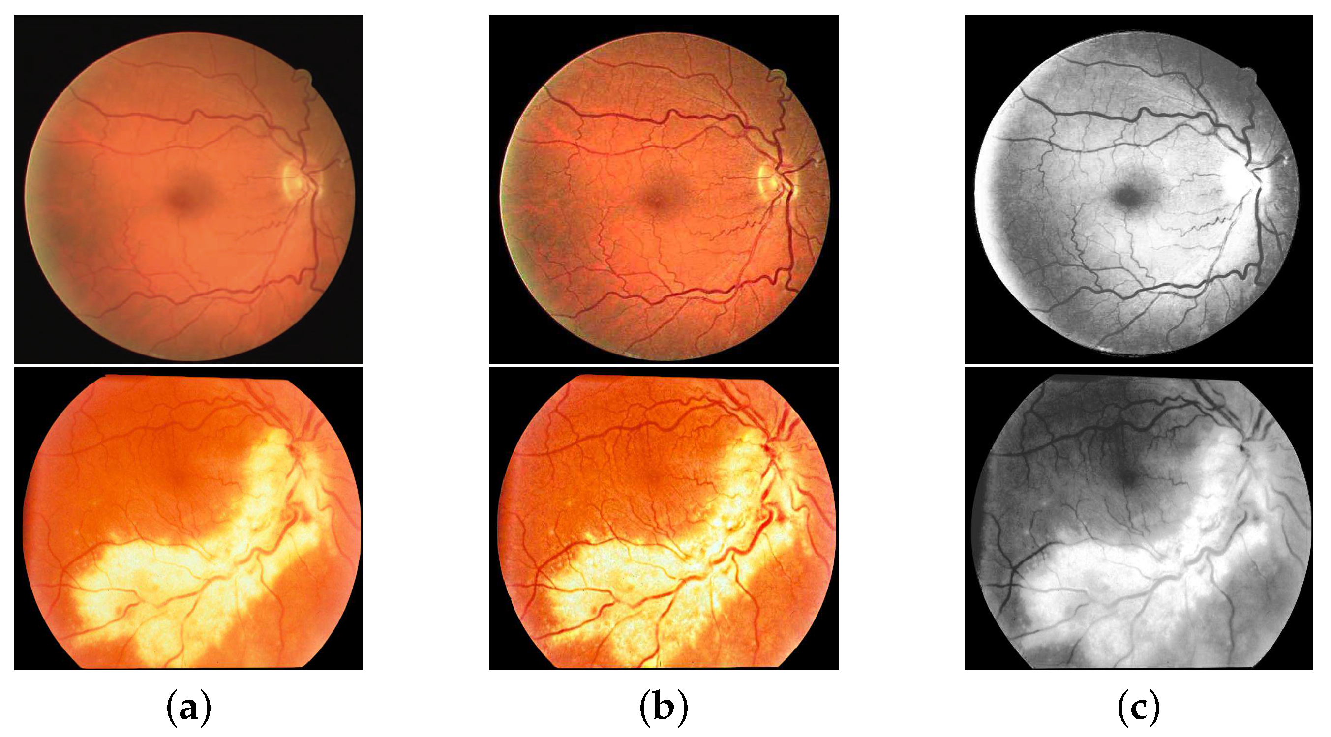
In this way, the gray scale of the vessel and background are stretched which is beneficial for the vessel separation. The comparison result of our enhancement operation is illustrated in Figure 2.
Horizontal flip: Image data offered in the dataset are often lacking paired fundus images (the left eye and corresponding right eye) which offer more information. We apply the horizontal flip operation on each fundus image to fill this gap and make the training data with more diversity.

2.2. Coarse Vessel Segmentation

Fundus vessel segmentation is the task of dense prediction in the computer vision filed which needs to assign each pixel in the image its corresponding category. It should take the pixel-level accuracy and multi-scale contextual reasoning into the consideration. Previous studies remold convolutional network for dense prediction by replacing fully-connected layers with fully-convolution layers, namely FCN. However, as image pixels are continuously changing, features extracted from small receptive field may not be obvious, that is to say, image information is unrepresentative. The traditional FCN used in the semantic segmentation tends to adopt pooling layers for expanding receptive field and reducing the output size. Because vessel segmentation is a end-to-end prediction, up-sampling layers are needed to restore the size of the image. Undoubtedly, this series of process will make images lose the resolution information. In view of this contradiction, we adopt dilated convolution (proposed in [26]) to replace the pooling layer in the original FCN, namely FG-FCN.
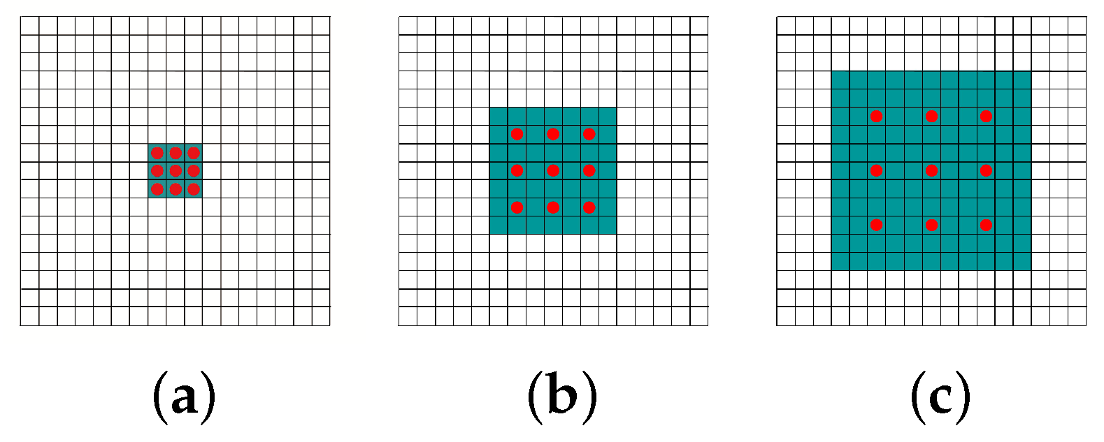
Dilated convolution is a novel mode of convolution which can apply the same filter (such as the 3 × 3 kernel used in our experiments) on different ranges using different dilation factors φ . It applies a kind of discrete convolution to fill zero values between every two valid points in the convolution kernel. In this way, it can have large receptive field without the increase of computation cost and retain more image semantic information. As the exemplary dilated convolution images shown in Figure 3, the red points mean the valid calculation ones in the convolution process and the weights of other points are set to be zero. The receptive field grows exponentially while the parameters increase linearly. Define the output of the layers as y [ i ] , and φ as the dilation rate. In one-dimensional case, dilated convolution with input x [ i ] is defined as follows. The w [ l ] here corresponds to the filter of length L.
y [ i ] = l = 1 L x [ i + φ · l ] w [ l ]
The structure of our FG-FCN is VGG16-style (stems from the schema of VGG16 [27]). We replace the pooling layers in VGG16 with dilated convolution layers and adjust the fully-connect layers to fully-convolution pattern for the requirement of pixel-level segmentation. As shown in Table 1, the dilation rates of FG-FCN are inspired by the concept of hybrid dilated convolution (HDC) [28]. This design of the dilation rate does not have a common divisor greater than one to avoid gridding effect [28], and it can make the perceived pixel of the kernel continuous at the same time. The alternative use of the traditional convolution and dilated convolution are aimed at dealing with vessels of different sizes. In this way, our network will avoid down-sampling operation and efficiently expand the network’s receptive field. Simultaneously, it can make full use of the raw information and keep more internal data structures compared to the original FCN. To train the network, we use the cross entropy loss and Adam optimizer [29] with learning rate = 0.0001. The ReLu activation function is employed to enhance the expression ability of the model.

2.3. Fine Optimization

CRF model is a graphical model which is widely used to take non-local correlations into account. For a given image X, CRF can model the conditional distribution of the category label and consider all the characteristics (i.e., shape, texture, color, location and edge) to obtain the global optimal solution. It still considers the label agreement between similar pixels which can overcome the shortcomings in remolding CNN for pixel-level labelling tasks. Many studies have used CRF to refine the coarse output of the network by regarding it as a post-processing step. It does not fully harness the superiority of the CRF as it cannot apply the weights of the former networks in CRF during the training stage. In our work, we adopt CRF as RNN [30] (see Algorithm 2) to integrate it with our FG-FCN for further optimizing its coarse output vessel map, namely CF-FCN, and it can train the weights and bias of FG-FCN and CRF as RNN simultaneously via back-propagation process.
CRF as RNN fully combines CNN and CRF in one unified framework, and each step accepts the information transferred from the former layers. Its target is to minimize a energy function given by:
E ( x ) = i ψ u ( x i ) + i < j ψ ( x i , x j ) ,
where ψ u ( x i ) is the unary terms measuring the cost of the pixel i belonging to the label x i , and the pairwise energy term ψ ( x i , x j ) is used to measure the cost of assigning labels x i , x j to pixels i, j simultaneously. Here, x i = 1 is the vessel pixel and x i = 0 is the non-vessel pixel. Due to the intractability of the E ( X ) , we implement the mean-field inference to approximate the CRF model as in [30]. After initializing the model with Q i ( l ) (i presents the ith pixel of the image and l (the label of it from 1 to the number of label L) obtained by a softmax function over the unary potentials U i ( l ) (the output of the final convolution layer of FG-FCN) for label l specific to each pixel i, the following four steps are applied. Z i used here is the partition function [31].
Message Passing: In this step, M Gaussian filters (a spatial kernel and a bilateral kernel used in our experiment) are applied on unary values Q i ( l ) . These filters are based on the characteristic such as the pixel locations to measure the relationship between the pixels.
Weighting Filter Outputs: To combine the result of the Gaussian filters used in last step, this part applies a 1 × 1 filter (similar to w ( m ) in Algorithm 2) on the output of the message passing phase. It is a weighted sum of the former two filters’ output for each label l and the error differentials can be computed through the back-propagation process.
Compatibility Transform: Compatibility Transform is a operation applied to consider the relationship between the similar pixels. It makes a fixed penalty μ ( l , l ) ( l , l are two labels) if pixels with similar properties are classified to different categories (l and l , respectively). This can be regarded as a convolution layer where the spatial receptive field of the filter is 1 × 1. We can obtain label compatibility function μ by learning the weights of this filter. The error differentials from the output of this step will be transferred to the input to carry out the update operation of the parameters.
Adding Unary Potentials: In this step, we subtract the output of compatibility transform element-wise from the former unary inputs U i ( l ) to transfer error differentials of this step.
Algorithm 2 CRF as RNN.
1:
Q i ( l ) 1 Z i e x p ( U i ( l ) ) for all i
2:
while not converged do
3:
     Q ˜ i ( m ) ( l ) j i k ( m ) ( f i , f j ) Q j ( l ) for all m
4:
     Q ˘ i ( l ) m w ( m ) Q ˜ i ( m ) ( l )
5:
     Q ^ i ( l ) l L μ ( l , l ) Q ˘ i ( l )
6:
     Q ˇ i ( l ) U i ( l ) Q ^ i ( l )
7:
end while

2.4. Morphological Post-Processing

The result of the neural network is prone to have discontinuous vessels (i.e., the pixels completely surrounded by vessel nodes, but are labeled as background pixels) or isolated nodes (i.e., the pixels misclassified as vessels, but the surrounding pixels are not) which need to be tackled. In the post-processing phase, we use morphological operations to enhance the binary output vessel maps generated by CF-FCN. The morphological closing operation is first used to fill the hole smaller than the structuring element (a disk of radius 10 is used in our experiment) in the vessel maps. For the isolated nodes, the acreage of these pixel area connected in the eight connectivity area is measured. We remove these misclassified pixel regions of the acreage below 100, and it will be reclassified as background pixels. In Figure 4, we show the exemplification for the performance of our post-processing. In Figure 4a,b, we can find the discontinuous vessels have been filled to a large degree. In addition, the isolated nodes that are smaller than our structuring element are removed.

3. Experiments

3.1. Dataset

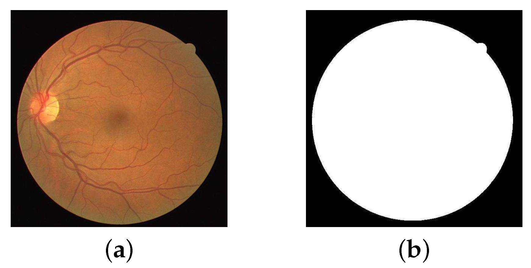
To validate our proposed method, we performed extensive experiments on four public fundus datasets, DRIVE, STARE, HRF and CHASE DB1, to evaluate the effectiveness of our method. Based on the consideration of the computation complexity and deficiency of the data, we crop these images into a quantity of 64 × 64 RGB patches to carry on our subsequent works. The mask is also provided for extracting the FOV of each fundus image, as shown in Figure 5. For those dataset (STARE and CHASE DB1) which do not offer masks for extracting FOV of the images, we created these masks for them, as described in [32]. We present a mask sample in DRIVE dataset in Figure 5.
DRIVE dataset: It is established to carry on comparative studies about vessel segmentation in retinal images. Each of them was digitalized to produce 565 × 584 images. There are all together 40 fundus images offered which have already been divided into training set (20 images) and testing set (20 images). Two manual observer segmentations are available in the dataset. All the ground-truth images we used in our experiments are the first human observer (the “gold standard”).
STARE dataset: The images and clinical data in STARE dataset were provided by the Shiley Eye Center at the University of California, San Diego, and by the Veterans Administration Medical Center in San Diego. The dataset contains 20 retinal images with manual segmentation results digitized of 700 × 605. We divide the data into training set and test set in equal proportion, and both contain healthy objects and pathological cases (the first five healthy and pathological images in the dataset for training and remaining for testing ).
HRF dataset: This database has been established by a collaborative research group to support comparative studies on automatic segmentation algorithms on retinal fundus images. It contains 15 high resolution images of healthy patients, 15 images of diabetic retinopathy patients and 15 images of glaucomatous patients. We chose the first eight images in each kind of cases for training and the others for testing. Gold standard fundus vessel segmentation results are offered by experienced experts. All images are digitized of 2336 × 3504.
CHASE DB1 dataset: It contains 28 high quality fundus images digitized of 999 × 960 collected from 14 school-age children’s left and right eyes. According to the convention, we used the first 20 images as training set and adopted the remaining images as test set. Data augmentation was also operated as narrated above.

3.2. Evaluation Metrics

In our work of fundus vessel segmentation, there are two possible labels: vessel and non-vessel. By comparing the vessel maps generated by our model with the ground-truth, four cases can be obtained: True Positive (TP), True Negative (NP), False Positive (FP) and False Negative (FN). TP is the pixel classified correctly as vessel and TN is the pixel classified correctly as non-vessel. FP is the pixel of background but misclassified as vessel, and FN is the pixel of vessel but misclassified as background in the vessel map. In our experiments, we used four measures to scrutinize our methods: Sensitivity ( S e ), Specificity ( S p ), Accuracy ( A c c ) and Area Under Receiver Operating Characteristic Curve ( A U C ). All evaluations were calculated only for pixels inside the FOV.
S e = T P T P + F N , S p = T N T N + F P
A c c = T P + T N T P + T N + F P + F N

3.3. Experimental Results

We scrutinized our proposed method on the test sets with 64 × 64 RGB patches, respectively. All manual segmentation we compared are from the first observer which served as the “gold standard”. For each fundus image in the test dataset, a binary vessel map can be obtained through our trained model. We calculated S e , S p , A c c and A U C indicators on the result to indicate our methods’ effectiveness. The implementation of our method is based on Tensorflow framework with NVIDIA GeForce GTX 1080 GPU.

3.3.1. The Improvement of the Data Quality

Instead of using green channel of original fundus images, we applied RGB fundus images with suitable enhancement operations. Although the green channel of the images own high contrast, colored images have inherent superiority of rich information. In our experiments, we applied green channel or RGB fundus images as the input of our CF-FCN with post-processing (CF-FCN-post) separately. As shown in Table 2, green channel images achieve S e of 0.6309, S p of 0.9891 and A c c of 0.9556, while RGB images obtain better performance with S e of 0.7941, S p of 0.9870 and A c c of 0.9634.

3.3.2. Comparison with the State-of-the-Art Works

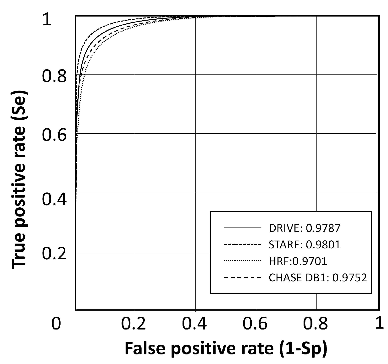
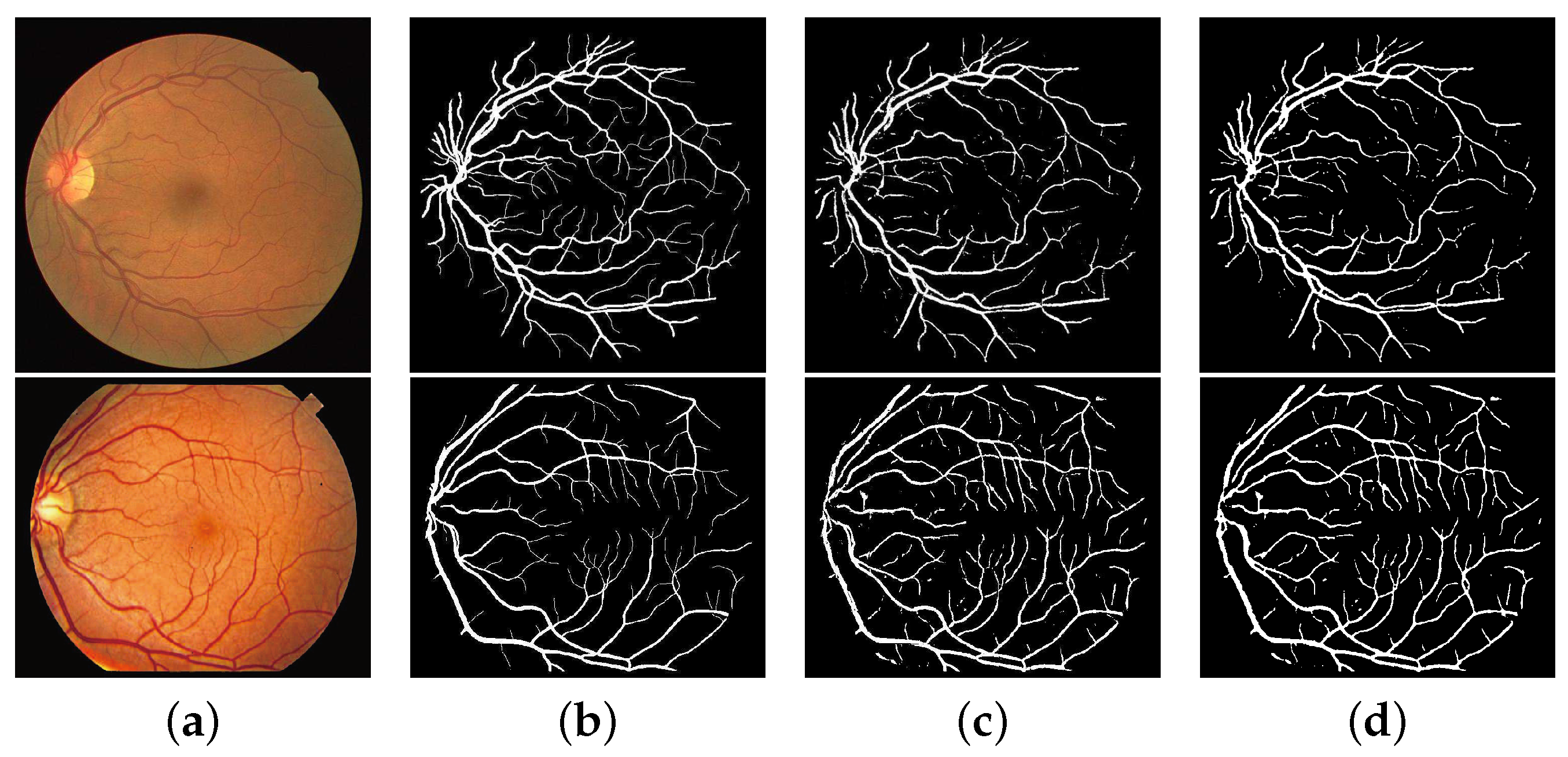
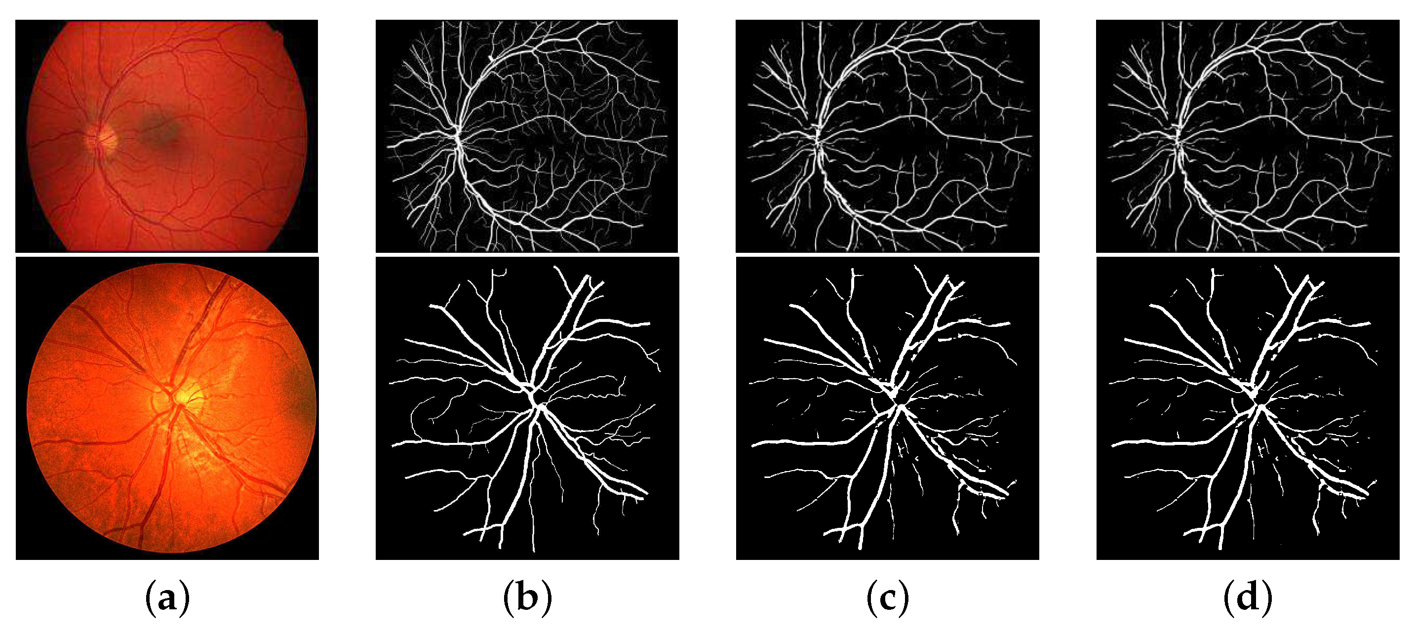
We verified our method by comparing it with state-of-the-art methods on DRIVE, STARE, HRF and CHASE DB1 datasets in Table 3, Table 4 and Table 5. To support our results, we show Confidence Interval (CI) on A c c in Table 6 and Receiver Operating Characteristic Curve (ROC) on datasets in Figure 6. In Table 3, we can see that the performance of our CF-FCN with post-processing achieves the best performance of S p (from the second best [7] 0.9838 to 0.9870) and A c c (from the second best [7] 0.9618 to 0.9634) on DRIVE dataset, and we get comparable result of Se with [8] on this dataset. Our method obtained an A U C of 0.9787. Similar results can be seen on STARE dataset in Table 4. Among other methods, our method achieved the best performance in terms of S p (0.9770), A c c (0.9628) and A U C (0.9801). Comparable result was obtained with regard to Se between our method and [6]. The binary vessel map results are in Figure 7 and Figure 8, which show our method works well on both healthy and pathological cases. To further validate the efficiency of our model, we tested it on HRF and CHASE DB1 datasets, as shown in Table 5. Compared with the listed methods, our model achieved the best performance of S e (0.7762), S p (0.9760), A c c (0.9608) and A U C (0.9701) on HRF dataset, and S e (0.7571), S p (0.9823), A c c (0.9664) and A U C (0.9752) on CHASE DB1 dataset. Further, we also show our segmentation results on HRF and CHASE DB1 datasets in Figure 9.

3.3.3. Improvement of the Network’s Structure

Different steps of our model: To show the effectiveness of the different steps of our proposed CF-FCN with post-processing, we compared the results by using traditional FCN (hereafter, FCN), FCN with dilated convolution but without CRF (FG-FCN), and CF-FCN-post. As shown in Table 7, compared to FCN, FG-FCN improves S e from 0.7110 to 0.7481, S p from 0.9750 to 0.9822, and A c c from 0.9508 to 0.9600, respectively. By further optimizing the coarse result of FG-FCN via CRF, the performance results of CF-FCN are further promoted to 0.7732 ( S e ), 0.9876 ( S p ) and 0.9623 ( A c c ). By using morphological enhancement as the post-processing in our CF-FCN in Figure 9, we get further performance improvement and total improvement up to 8.31% ( S e ), 1.2% ( S p ), and 1.26% ( A c c ) compared to FCN on DRIVE dataset. Examples of the binary vessel map of different steps are shown in Figure 10. In this figure, we can see that more detailed information of the vessels are kept in FG-FCN and CF-FCN compared to FCN.
Parameters adjustment of our model: We have elaborated in Section 2.2 that our designed dilated parameters can avoid efficiently gridding problem. Through Figure 11b, it can be clearly seen that gridding problem exists in the vessel segmentation result using casual dilated parameters (using dilated rate increasing proportionally such as series of 1, 2, 4 and 8). Although it can be a little bit better in the latter iterations in Figure 11c, there are more background pixels misclassified as vessel pixels than in Figure 11d caused by poor results from former iterations. In our work, we used dilated rates 1, 2, 3, 5 and 7 in order according to Table 1, which validated its efficacy through our comparison experiments. In Figure 11d, our vessel segmentation result performs better without the existing of gridding problem.
Comparison of similar works: To validate our improvement of dealing with the problem of the loss of resolution, we compared our CF-FCN with post-processing with some typical similar networks (U-net and Deeplab v3 ) also focused on this aspect. As shown in Table 8, our CF-FCN-post shows improvement compared to U-net in the aspect of S e from 0.7912 to 0.7941, S p from 0.9704 to 0.9870, and A c c from 0.9561 to 0.9634. Compared with Deeplab v3, our CF-FCN-post still works better than it, as shown in Table 8.

4. Discussion and Conclusions

In this paper, we propose a CF-FCN with post-processing to address the problem of fundus vessel segmentation. Our methods retain more internal information and make full use of the data. At the same time, we better consider the non-local correlations through optimizing the coarse output of our FG-FCN. After extracting fundus vessel tree using our method, it can be used for the quantitative analysis of patients or for biometric identification due to its uniqueness.
To the best of our knowledge, we are the first to apply this kind of CF-FCN accompanying with necessary and efficient pre- and post-processing operations in the field of fundus vessel segmentation. The experimental results display that our method surpasses reported state-of-the-art methods in terms of sensitivity, specificity and accuracy on the publicly-available datasets DRIVE, STARE, HRF and CHASE DB1.
Since vessels’ size vary greatly a fundus image, the characteristics of each kind of vessel are often overlooked. For example, large receptive fields are friendly to the large vessels but not suitable for tiny vessels. However, small ones are not a good choice for non-local information. In our method, we tend to apply a balanced approach to take large and small vessels into the consideration at the same time. To improve our methods in the future, we will explore some multi-stream methods which solve different vessels in different streams to better address tiny and large vessels separately.

Author Contributions

J.L. and Y.X. conceived and designed the experiments; Y.X. performed the experiments and analyzed the data; M.C. validate our methods and do the data collections; J.L. wrote the paper; Y.L. is the person in charge of the research.

Funding

This research was funded by National Natural Science Foundation of China (NSFC) under grant No. 61806147, Shanghai Natural Science Foundation under Grant No. 18ZR1441200 and Fundamental Research Funds for the Central Universities under Grant No. 22120180012.

Conflicts of Interest

The authors declare no conflict of interest.

References

  1. Li, J.; Hu, Q.; Imran, A.; Zhang, L.; Yang, J.; Wang, Q. Vessel Recognition of Retinal Fundus Images Based on Fully Convolutional Network. In Proceedings of the 2018 IEEE 42nd Annual Computer Software and Applications Conference (COMPSAC), Tokyo, Japan, 23–27 July 2018; pp. 413–418. [Google Scholar] [CrossRef]
  2. Poplin, R.; Varadarajan, A.V.; Blumer, K.; Liu, Y.; Mcconnell, M.V.; Corrado, G.S.; Peng, L.; Webster, D.R. Predicting Cardiovascular Risk Factors from Retinal Fundus Photographs using Deep Learning. arXiv, 2017; arXiv:1708.09843. [Google Scholar]
  3. Fraz, M.M.; Remagnino, P.; Hoppe, A.; Uyyanonvara, B.; Rudnicka, A.R.; Owen, C.G.; Barman, S.A. Blood vessel segmentation methodologies in retinal images—A survey. Comput. Methods Prog. Biomed. 2012, 108, 407–433. [Google Scholar] [CrossRef] [PubMed]
  4. Azzopardi, G.; Strisciuglio, N.; Vento, M.; Petkov, N. Trainable COSFIRE filters for vessel delineation with application to retinal images. Med. Image Anal. 2015, 19, 46–57. [Google Scholar] [CrossRef] [PubMed] [Green Version]
  5. Jiang, X.; Mojon, D. Adaptive local thresholding by verification-based multithreshold probing with application to vessel detection in retinal images. IEEE Trans. Patt. Anal. Mach. Intell. 2015, 25, 131–137. [Google Scholar] [CrossRef]
  6. Ramalho, G.L.B.; Ramalho, G.L.B.; Veras, R.M.S.; Veras, R.M.S.; Medeiros, F.N.S. An unsupervised coarse-to-fine algorithm for blood vessel segmentation in fundus images. Expert Syst. Appl. 2017, 78, 182–192. [Google Scholar] [CrossRef]
  7. Zhu, C.; Zou, B.; Xiang, Y.; Cui, J.; Hui, W.U. An ensemble retinal vessel segmentation based on supervised learning in fundus images. Chin. J. Electron. 2016, 25, 503–511. [Google Scholar] [CrossRef]
  8. Xiao, Z.; Wang, M.; Zhang, F.; Geng, L.; Wu, J.; Su, L.; Tong, J. Retinal vessel segmentation based on adaptive difference of Gauss filter. In Proceedings of the IEEE International Conference on Digital Signal Processing, Beijing, China, 16–18 October 2016; pp. 15–19. [Google Scholar]
  9. Staal, J.; Abramoff, M.D.; Niemeijer, M.; Viergever, M.A.; Van Ginneken, B. Ridge-based vessel segmentation in color images of the retina. IEEE Trans. Med. Imaging 2004, 23, 501–509. [Google Scholar] [CrossRef] [PubMed]
  10. Hoover, A.D.; Kouznetsova, V.; Goldbaum, M. Locating blood vessels in retinal images by piecewise threshold probing of a matched filter response. IEEE Trans. Med. Imaging 2000, 19, 203–210. [Google Scholar] [CrossRef] [PubMed] [Green Version]
  11. Budai, A.; Bock, R.; Maier, A.; Hornegger, J.; Michelson, G. Robust vessel segmentation in fundus images. Int. J. Biomed. Imaging 2013, 2013, 154860. [Google Scholar] [CrossRef] [PubMed]
  12. Fraz, M.; Remagnino, P.; Hoppe, A.; Uyyanonvara, B.; Rudnicka, R.A.; Owen, G.C.; Barman, S.A. An Ensemble Classification-Based Approach Applied to Retinal Blood Vessel Segmentation. IEEE Trans. Biomed. Eng. 2012, 59, 2538–2548. [Google Scholar] [CrossRef] [PubMed] [Green Version]
  13. Singh, D.; Dharmveer, S.; Singh, B. A new morphology based approach for blood vessel segmentation in retinal images. In Proceedings of the 2014 Annual IEEE India Conference (INDICON), Pune, India, 11–13 December 2014; pp. 1–6. [Google Scholar]
  14. Dash, J.; Bhoi, N. A thresholding based technique to extract retinal blood vessels from fundus images. Future Comput. Inf. J. 2017, 2, 103–109. [Google Scholar] [CrossRef]
  15. Odstrcilik, J.; Kolar, R.; Budai, A.; Hornegger, J. Retinal vessel segmentation by improved matched filtering: Evaluation on a new high-resolution fundus image database. IET Image Process. 2013, 7, 373–383. [Google Scholar] [CrossRef]
  16. Osareh, A.; Shadgar, B. Automatic blood vessel segmentation in color images of retina. Iran. J. Sci. Technol. Trans. B 2009, 33, 191–206. [Google Scholar]
  17. Havaei, M.; Davy, A.; Warde-Farley, D.; Biard, A.; Courville, A.; Bengio, Y.; Pal, C.; Jodoin, P.; Larochelle, H. Brain Tumor Segmentation with Deep Neural Networks. Med. Image Anal. 2017, 35, 18–31. [Google Scholar] [CrossRef] [PubMed]
  18. Dan, C.C.; Giusti, A.; Gambardella, L.M.; Schmidhuber, J. Deep neural networks segment neuronal membranes in electron microscopy images. Adv. Neural Inf. Process. Syst. 2012, 25, 2852–2860. [Google Scholar]
  19. Li, Q.; Feng, B.; Xie, L.P.; Liang, P.; Zhang, H.; Wang, T. A cross-modality learning approach for vessel segmentation in retinal images. IEEE Trans. Med. Imaging 2016, 35, 109–118. [Google Scholar] [CrossRef] [PubMed]
  20. Song, J.; Boreom, L. Development of automatic retinal vessel segmentation method in fundus images via convolutional neural networks. In Proceedings of the 2017 39th Annual International Conference of the IEEE Engineering in Medicine and Biology Society (EMBC), Seogwipo, Korea, 11–15 July 2017; pp. 681–684. [Google Scholar] [CrossRef]
  21. Liskowski, P.; Krawiec, K. Segmenting retinal blood vessels with deep neural networks. IEEE Trans. Med. Imaging 2016, 35, 2369–2380. [Google Scholar] [CrossRef] [PubMed]
  22. Fu, H.; Xu, Y.; Lin, S.; Wong, D.W.K.; Liu, J. DeepVessel: Retinal Vessel Segmentation via Deep Learning and Conditional Random Field. In Proceedings of the International Conference on Medical Image Computing and Computer-Assisted Intervention, Quebec City, QC, Canada, 11–13 September 2017; pp. 132–139. [Google Scholar]
  23. Dasgupta, A.; Singh, S. A fully convolutional neural network based structured prediction approach towards the retinal vessel segmentation. In Proceedings of the ISBI, Melbourne, VIC, Australia, 18–21 April 2017; pp. 248–251. [Google Scholar] [CrossRef]
  24. Li, Q.; Xie, L.; Zhang, Q.; Qi, S.; Liang, P.; Zhang, H.; Wang, T. A supervised method using convolutional neural networks for retinal vessel delineation. In Proceedings of the 2015 8th International Congress on Image and Signal Processing (CISP), Shenyang, China, 14–16 October 2015; pp. 418–422. [Google Scholar]
  25. Fu, H.; Xu, Y.; Wong, D.W.K.; Liu, J. Retinal vessel segmentation via deep learning network and fully-connected conditional random fields. In Proceedings of the 2016 IEEE 13th International Symposium on Biomedical Imaging (ISBI), Prague, Czech, 13–16 April 2016; pp. 698–701. [Google Scholar]
  26. Yu, F.; Koltun, V. Multi-scale context aggregation by dilated convolutions. arXiv, 2015; arXiv:1511.07122. [Google Scholar]
  27. Simonyan, K.; Zisserman, A. Very deep convolutional networks for large-scale image recognition. arXiv, 2014; arXiv:1409.1556. [Google Scholar]
  28. Wang, P.; Chen, P.; Yuan, Y.; Liu, D.; Huang, Z.; Hou, X.; Cottrell, G. Understanding convolution for semantic segmentation. WACV 2017, 2018, 1451–1460. [Google Scholar] [CrossRef]
  29. Kingma, D.P.; Ba, J. Adam: A method for stochastic optimization. arXiv, 2014; arXiv:1412.6980. [Google Scholar]
  30. Zheng, S.; Jayasumana, S.; Romeraparedes, B.; Vineet, V.; Su, Z.; Du, D.; Huang, C.; Torr, P.H.S. Conditional random fields as recurrent neural networks. In Proceedings of the 2015 IEEE International Conference on Computer Vision (ICCV), Santiago, Chile, 7–13 December 2015; pp. 1529–1537. [Google Scholar]
  31. Lafferty, J.D.; Mccallum, A.; Pereira, F.C.N. Conditional Random Fields: Probabilistic Models for Segmenting and Labeling Sequence Data. In Proceedings of the Eighteenth International Conference on Machine Learning, Williamstown, MA, USA, 28 June–1 July 2001; pp. 282–289. [Google Scholar]
  32. Soares, J.V.B.; Leandro, J.J.G.; Cesar, R.M.; Jelinek, H.F.; Cree, M.J. Retinal vessel segmentation using the 2-D gabor wavelet and supervised classification. IEEE Trans. Med. Imaging 2006, 25, 1214–1222. [Google Scholar] [CrossRef] [PubMed] [Green Version]
  33. Ngo, L.; Han, J.H. Multi-level deep neural network for efficient segmentation of blood vessels in fundus images. Electron. Lett. 2017, 53, 1096–1098. [Google Scholar] [CrossRef]
  34. Niemeijer, M.; Ginneken, B.V.; Loog, M. Comparative study of retinal vessel segmentation methods on a new publicly available database. In Proceedings of the Medical Imaging 2004: Image Processing, San Diego, CA, USA, 12 May 2004; pp. 648–656. [Google Scholar] [CrossRef]
  35. Fraz, M.M.; Barman, S.A.; Remagnino, P.; Hoppe, A.; Basit, A.; Uyyanonvara, B.; Rudnicka, A.R.; Owen, C.G. An approach to localize the retinal blood vessels using bit planes and centerline detection. Comput. Meth. Prog. Biomed. 2017, 108, 600–616. [Google Scholar] [CrossRef] [PubMed]
  36. Budai, A.; Hornegger, J.; Michelson, G. Multiscale approach for blood vessel segmentation on retinal fundus images. Arvo Meet. Abst. 2009, 50, 325. [Google Scholar]
  37. Ronneberger, O.; Fischer, P.; Brox, T. U-net: Convolutional networks for biomedical image segmentation. In Proceedings of the International Conference on Medical Image Computing and Computer-Assisted Intervention, Munich, Germany, 5–9 October 2015; pp. 234–241. [Google Scholar]
  38. Chen, L.C.; Papandreou, G.; Schroff, F.; Adam, H. Rethinking Atrous Convolution for Semantic Image Segmentation. arXiv, 2017; arXiv:1706.05587. [Google Scholar]
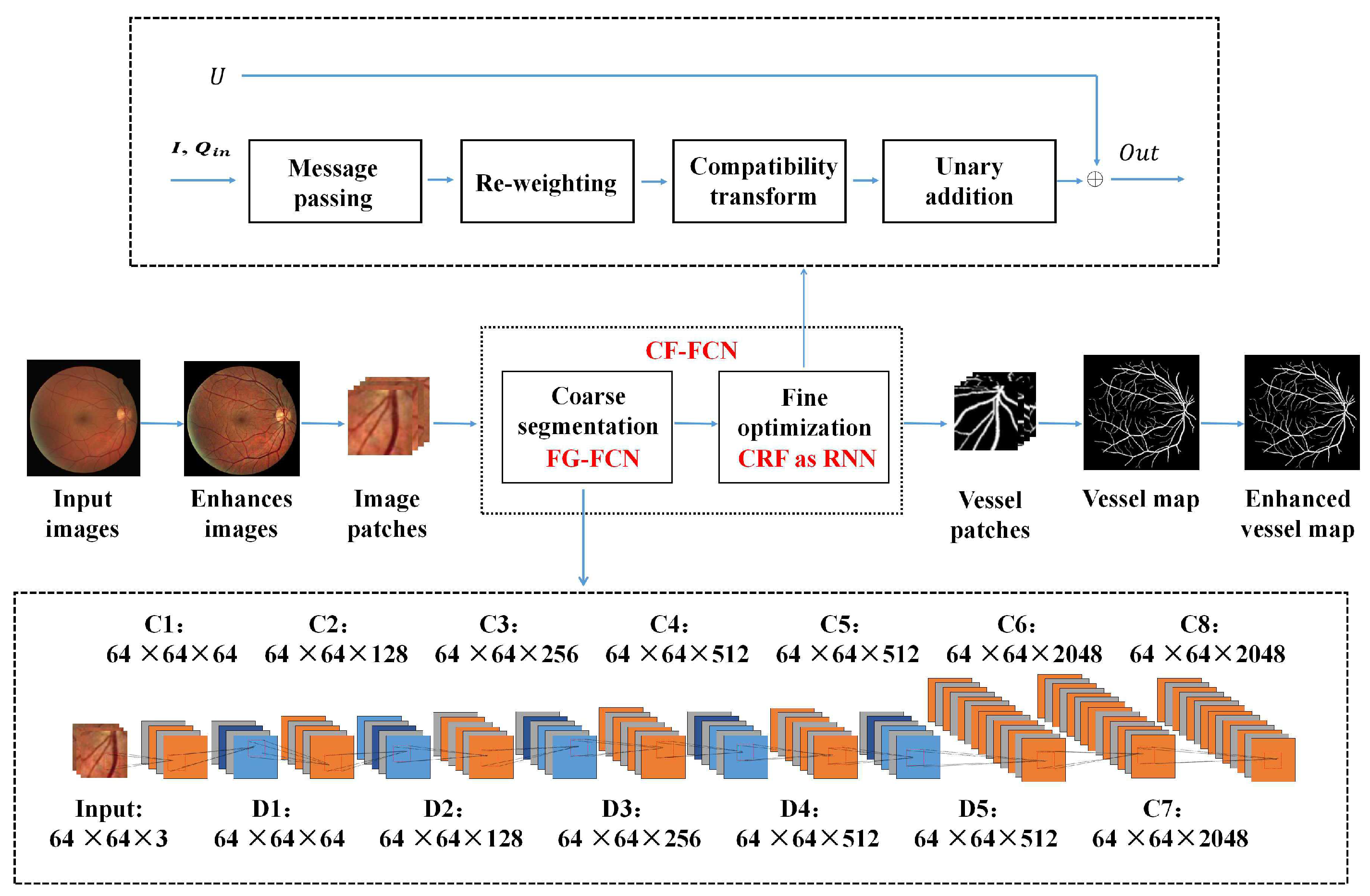
Figure 1. The overall structure of our method (CF-FCN with post-processing). We use FG-FCN to refer to traditional FCN with dilated convolution but without CRF. The top line of the figure is the steps of CRF as RNN. In bottom line of the figure is the details of FG-FCN. C i represents the tied convolution layers (the numbers of tied convolution layers are shown in Table 1). The final three C i layers are the single convolution layers. D i means dilated convolution layers. All layers are denoted as “width × height × number of feature maps”.
Symmetry 10 00607 g001
Figure 2. The fist line is the fundus image in DRIVE dataset. The second line is the fundus image in STARE dataset: (a) the original fundus image; (b) the fundus image with contrast enhancement on (a); and (c) the green channel image of (a). It can be clearly seen that the vessels are more prominent in (b) which retain more internal information than (a,c).
Symmetry 10 00607 g002
Figure 3. (a) The dilated convolution with the rate of 1; (b) the dilated convolution with the rate of 2; and (c) the dilated convolution with the rate of 3.
Symmetry 10 00607 g003
Figure 4. Comparison of the fundus vessel images before and after our post-processing: (a) the images before the operation and we circle the region in red to focus; and (b) the images after the operation of (a). The same regions are circled in red to compare the performance of our post-processing. The first line is the sample in DRIVE dataset. The second line is the sample in STARE dataset.
Symmetry 10 00607 g004
Figure 5. (a) The fundus image in DRIVE dataset; and (b) the mask of (a).
Symmetry 10 00607 g005
Figure 6. ROC of our methods on the four datasets.
Symmetry 10 00607 g006
Figure 7. Segmentation results of our method. The first line is the healthy objects in DRIVE dataset. The second line is the healthy case in STARE dataset: (a) is the fundus image; (b) is the manual segmentation; (c) is the vessel map generated by our CF-FCN; and (d) is the enhanced result of CF-FCN with morphological post-processing.
Symmetry 10 00607 g007
Figure 8. Segmentation results of our method. The first line is the pathological objects in DRIVE dataset. The second line is the pathological case in STARE dataset: (a) the fundus image; (b) the manual segmentation; (c) the vessel map generated by our CF-FCN; and (d) the enhanced result of CF-FCN with morphological post-processing.
Symmetry 10 00607 g008
Figure 9. Segmentation results of our method. The first line is the objects in HRF dataset. The second line is the case in CHASE DB1 dataset: (a) the fundus image; (b) the manual segmentation; (c) the vessel map generated by our CF-FCN; and (d) the enhanced result of CF-FCN with morphological post-processing.
Symmetry 10 00607 g009
Figure 10. Segmentation comparison with different steps of the proposed models on DRIVE dataset: (a) the fundus image; (b) the output of FCN; (c) the vessel map result of FG-FCN; and (d) the result of CF-FCN.
Symmetry 10 00607 g010
Figure 11. (a) The ground-truth of the fundus vessel segmentation; (b) the vessel images using the casual dilated parameter in the front iteration; (c) the vessel images using the casual dilated parameter in the iteration with stable loss; and (d) the vessel images using the our designed dilated parameter with stable loss.
Symmetry 10 00607 g011
Table 1. The parameters configuration of our FG-FCN. Conv represents the convolution layers, and DConv represents the dilated convolution layers. Maps column refers to the number of the feature maps in this layer. In Para. column, the stride parameters are used in convolution layers and dilation rate is applied instead of stride factor.
LayerTypeMapsKernelPara.LayerTypeMapsKernelPara.
0Input3--11Conv5123 × 31
1Conv643 × 3112Conv5123 × 31
2Conv643 × 3113Conv5123 × 31
3DConv643 × 3114DConv5123 × 35
4Conv1283 × 3115Conv5123 × 31
5Conv1283 × 3116Conv5123 × 31
6DConv1283 × 3217Conv5123 × 31
7Conv2563 × 3118DConv5123 × 37
8Conv2563 × 3119Conv20487 × 71
9Conv2563 × 3120Conv20481 × 11
10DConv2563 × 3321Conv20481 × 11
Table 2. Performance comparison with different channels as input of CF-FCN-post on DRIVE dataset.
TypeSeSpAcc
Green channel images0.63090.98910.9556
RGB images0.79410.98700.9634
Table 3. Comparison with state-of-the-art methods on DRIVE dataset.
TypeMethodSeSpAccAUC
UnsupervisedSingh et al. [13]0.71380.98010.9460-
methodsOdstrcilik et al. [15]0.70600.96930.93400.9519
Xiao et al. [8]0.81270.97860.9580-
Neto et al. [6]0.78060.96290.8718-
SupervisedLi et al. [19]0.75690.98160.95270.9738
methodsSong et al. [20]0.75010.97950.9499-
Ngo et al. [33]0.74640.98360.95330.9752
Zhu et al. [7]0.74620.98380.9618-
Li et al. [24]0.76590.97970.9522-
CF-FCN-post0.79410.98700.96340.9787
Table 4. Comparison with state-of-the-art methods on STARE dataset.
TypeMethodSeSpAccAUC
UnsupervisedNiemeijer et al. [34]0.68980.96960.9417-
methodsOdstrcilik et al. [15]0.78470.95120.93410.9569
Xiao et al. [8]0.76410.97570.9569-
Neto et al. [6]0.83440.94430.8894-
SupervisedFraz et al. [12]0.75480.97630.95340.9768
methodsFu et al. [25]0.7140-0.9545-
Fraz et al. [35]0.73110.96800.9442-
Soares et al. [32]0.71030.97370.9480-
CF-FCN-post0.80900.97700.96280.9801
Table 5. Comparison with state-of-the-art methods on HRF and CHASE DB1 dataset.
DatasetMethodSeSpAccAUC
HRFOdstrcilik et al. [15]0.77410.96690.94940.9667
Budai et al. [36]0.70990.97450.9481-
CF-FCN-post0.77620.97600.96080.9701
CHASE DB1Li et al. [19]0.75690.98160.95270.9712
Fu et al. [22]0.7130-0.9489-
CF-FCN-post0.75710.98230.96640.9752
Table 6. CI of Acc on datasets.
DatasetsDRIVESTAREHRFCHASE DB1
CI[0.9612, 0.9641][0.9620, 0.9679][0.9584, 0.9612][0.9624, 0.9705]
Table 7. Performance comparison with different steps of the proposed models on DRIVE dataset.
StepSeSpAcc
FCN0.71100.97500.9508
FG-FCN0.74810.98220.9600
CF-FCN0.77320.98760.9623
CF-FCN-post0.79410.98700.9634
Table 8. Performance comparison with other similar networks on DRIVE dataset.
NetworkSeSpAcc
U-Net [37]0.79120.97040.9561
Deeplab v3 [38]0.77110.97770.9595
CF-FCN-post0.79410.98700.9634