The α-Representation Inexact T2 Fuzzy Sets Programming Model for Water Resources Management of the Southern Min River Basin under Uncertainty

Abstract

In this study, a new α-representation of the inexact T2 fuzzy sets programming model (α-RITF2SP) is proposed for water resources planning under uncertainties. The developed model is a hybrid of inexact type-2 (T2) fuzzy sets (FSs) optimal programming based on α-cuts and α-planes (z-slices) algorithms, and both can be used in problems of water resource management without a loss of generality. Therefore, this novel method represents a complementary method to combine both of these algorithms to make inexact T2FSs methods easier and faster for users under uncertainties. This method provides not only a reduction in computations when computing fuzzy functions, but also a map of the primary variable of T2FSs in the secondary membership function. The α-RITF2SP is applied to a real case study of the operation of water resource systems in the southern Min River basin that involves three cities: Xiamen, Zhangzhou, and Quanzhou. The results of the water allocations and benefits have been analyzed. The symptoms of results indicate the higher profit with a higher wastewater treatment rate. It also represents that this model has enhanced abilities and it is relevant and practical as well as can serve as a guide for the development of this regional economy.

1. Introduction

With the development of the economy and the increase in the population, the demand for water resources is increasing. However, due to the irrational exploitation and unitization of water resources, many countries, especially developing countries, such as India, China, Mexico, and South Africa, experience different levels of water shortage. In response to the issue of water resource allocation and optimization, many scholars have studied and addressed this issue based on operation research studies. To date, these studies can be divided into linear programming (LP) and nonlinear programming (NLP) according to the function relationships. Similarly, these studies can be distinguished by crisp models and uncertain models. However, uncertainty is an important factor that could highly affect water resources allocation [1]. For example, there is a peak period and bottom period for just one day of water consumption; the seasonality of water resources is also an important factor of volatility. In fact, very few water resources remain at a constant amount. In addition, other human controlled conditions of the social economy and environmental policy are constantly changing year to year. These issues require uncertain methods to address such complex inputs. Consequently, inexact, fuzzy, and stochastic models or algorithms have been preferred to consider uncertainty beyond the conventional planning methods. In agricultural water resource management, uncertainty is frequently considered because of incomplete data records. Therefore, this study mainly provides a relatively in-depth understanding of water resources management of local agriculture combined with discussions of the relevant regulations and various related optimal planning studies in the world; the results of this study can provide powerful decision support for water resources allocation in the southern Min River basin. Moreover, a new α-representation fuzzy sets (FS) optimization model is proposed in this study. This study also provides a valuable analysis of the economic development and optimal utilization of the limited water resources in this area.

Regarding the uncertainty of water resources management, many research studies have been conducted on this issue. In 2000, Huang et al. [2] developed an inexact two-stage stochastic programming (ITSP) model for water resources management. This algorithm can reflect not only uncertainties that are expressed as probability distributions, but also those made available as interval numbers. In 2005, Maqsood et al. [3] presented an interval-parameter fuzzy two-stage stochastic programming (IFTSP) method for the planning of water resources management; the authors used an optimization framework to represent predefined water policies and then applied discrete interval numbers with the possibility and probability distribution in their solution process, resulting in an efficient policy to use the water. Li et al. [4], in 2008, developed an inexact multistage stochastic integer programming (IMSIP) method for the management of water resources; this method can use probabilities and dynamics methods to reflect a complete scenario set over a multistage context. In 2017, Liu et al. [5] introduced a two-stage regional multi-water source allocation model (TRMSA) to determine the water supply that consisted of surface water, ground water, and transit water. This model can optimize water supply for a shortage year of water and satisfy requirements of each targets in the water systems. In general, these studies could address uncertainty by using interval numbers, probability degrees and the two-stage programming (TSP) model; however, none of the aforementioned studies considered the type-2 (T2) fuzzy sets model, which has been used extensively to capture linguistic uncertainty in decision-making problems [6].

Recently, studies of the optimal fuzzy linear programming have been conducted. As an extension of the conventional FS concept, the higher levels of fuzzy sets, the T2FSs, have been coupled into the water model to handle more uncertainty and hence to produce more accurate and robust results [7,8] because of the introduction of the T2FSs into the optimal process. This approach has been widely used because T2FSs can consider more uncertainty in various areas. Çebi and Otay [9] proposed an approach using the interval T2FSs method. The suggested approach has been applied to a site selection problem of a cement factory. The interval T2FSs method is a special version of the general T2FSs method. IT2FSs are the most applicable T2FSs because of the reduced computational effort in comparison with normal T2FSs. Mehdi et al. [10] integrated both IT2FSs and multiple criteria decision making (MCDM) problems, in which there is done an intensive research concerning the application of other fuzzy sets to solve it [11,12,13,14,15]. This MCDM can be transferred into a new approach based on the weight aggregated sum product assessment (WASPAS) method. The WASPAS method can help increase the stability of the uncertain issues. Runkler et al. [16] extended type 1 fuzzy sets (T1FSs) to IT2FSs in a decision-making situation by considering the risk associated with the decision making; they revealed that the T2 approach contains a larger solution space to enable a better decision. Suo et al. [17] developed a T2 fuzzy chance-constrained programming (TFCP) method for energy systems planning under uncertainty. Roy and Bhaumik [18] considered a triangular T2FSs intuitionistic fuzzy matrix game to treat policy-management toward the free and fair accession of water against its limited resources. In their study, the T2FSs mathematic programming reduced the time of calculation to obtain the final results in water resource management.

However, these aforementioned research studies had obvious limitations in terms of the reduction of the calculated intensity and accuracy of T2FSs. These studies cannot reflect the features of the primary variable of a T2FSs, which is especially useful in the problems of the engineering planning. If the application of T2FSs is to reflect the “level of uncertainty” of a problem, but the solution process in the engineering scope does oversimplify the feature of the T2FSs regarding the operability. The definitions of T2FSs are given by Mendel [19]. $\tilde{A}$ is a mapping $\tilde{A}=X\to F\left(\left[0,1\right]\right)$ defined over a nonempty universe, where $A$ is a linguistic word, $\tilde{A}$ indicates the uncertainty of $A$, and $F_1\left(X\right)$ is the class of all FSs over the $X$; the corresponding $F_2\left(X\right)$ is the class of all T2FSs over the $X$. Previously, the α-cut, which is defined as ${}^{a}A=\left\{x|{\mu }_A(x)\ge \alpha \right\}$, was the most commonly used solution method for functions of T2FSs, especially in the interval type-2 fuzzy sets (IT2FSs) problems. The α-cut mapping ${}^{\alpha }\tilde{A}$ is the union of all fulfilled requirements of the FSs. However, this method is incapable of reflecting the uncertainty of the third dimension membership function of the T2FSs. Consequently, the α-plane was introduced for a general T2FS [20]. The α-plane denotes a T2 fuzzy set of ${\tilde{A}}_{\alpha }$, which is the union of all first memberships of $\tilde{A}$, whose secondary grades are greater or equal to α $\left(0\le \alpha \le 1\right)$. Both methods are usually given by experts who may use their perceptions. The flaws are very obvious in these complex engineering problems. Therefore, based on these studies either on α-cuts or α-planes, none of the algorithms can precisely reflect the characteristic of the general T2FSs. Thus, although the decision managers are willing to receive a higher profit in the existing water resources, the results that were obtained from uncertain analysis based on experts’ experience often lead to more confusion and subjectivity. The advantages of applying T2FSs in the practical problems have not been proved by optimal controllers [21]. The T2FSs are better able to handle uncertainties than the traditional type-1 fuzzy sets. Thus, to achieve a better solution, the concepts of α-cuts and α-planes can be combined and defined to produce a small uncertainty area of the decision space. The inexact T2FSs programming algorithm containing the α-representation can achieve more accurate results for fuzzy optimization and fuzzy equations.

This study aims to develop an α-representation model that offers advantages on both α-cuts and α-planes/z-slices for the general T2FSs as the complementary measures. The α-representation method can combine α-cuts and α-planes into a smaller space over a particular $x\in X$. This double cut algorithm, which corresponds to the cuts both in two-dimensional and three-dimensional spaces, can certainly produce a small uncertainty decision area. Clearly, the larger cuts of the α-cut and z-slice will result in less uncertainty. Thus, the union of all $x\in X$ for cut and plane provides a better result for the decision maker. The α-RITF2S programming model can integrate the α-representation method in a general optimal framework. This new innovative method is capable of reflecting the uncertainty of the parameter constraints expressed as T2FSs and offers an accurate decision support. This developed model will be applied to a real case study of management of the irrigation water system of the southern Min River Basin located in southeastern China. The study is based on the predecessor’s study of fuzzy linear programming and inexact linear programming methods, and the developed model is combined with the carrying capacity of agricultural environmental resources. This study attempts to establish a water system allocation model with uncertain factors that provides a valuable reference for the sustainable development of the Southern Min river basin. The results from the α-RITF2S programming model support the less uncertain results that were obtained from the in-depth uncertainty among volatility of water resources, the changes in supply and demand, and the perceptions between water authority and users; the results will benefit the local residents and descendants in this area for a long time and provide a reference for environmentally sustainable development in other regions. However, in this paper, many factors are considered to reflect the actual situation in this area; as a result, a certain one-sidedness may exist. The participants should make the corresponding adjustments according to the specific conditions when referring to the results of this paper.

2. Methodology

Consider a problem in which a water manager is charged with supplying water from various sources during a dry season to multiple users. The users are expanding their activities and determine how much water they can expect. If an insufficient amount of water is available, then they will curtail their expansion plans. In a real-life problem, parameter B on the right side of model denotes a higher level of an uncertain situation that can be treated as a T2FS. Prior to proposing the α-RITF2S programming model, the following definition gives the background information of Type-2 fuzzy sets (T2FSs).

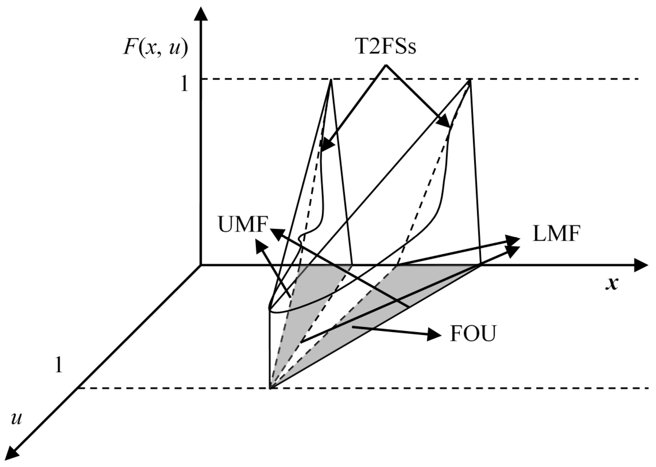
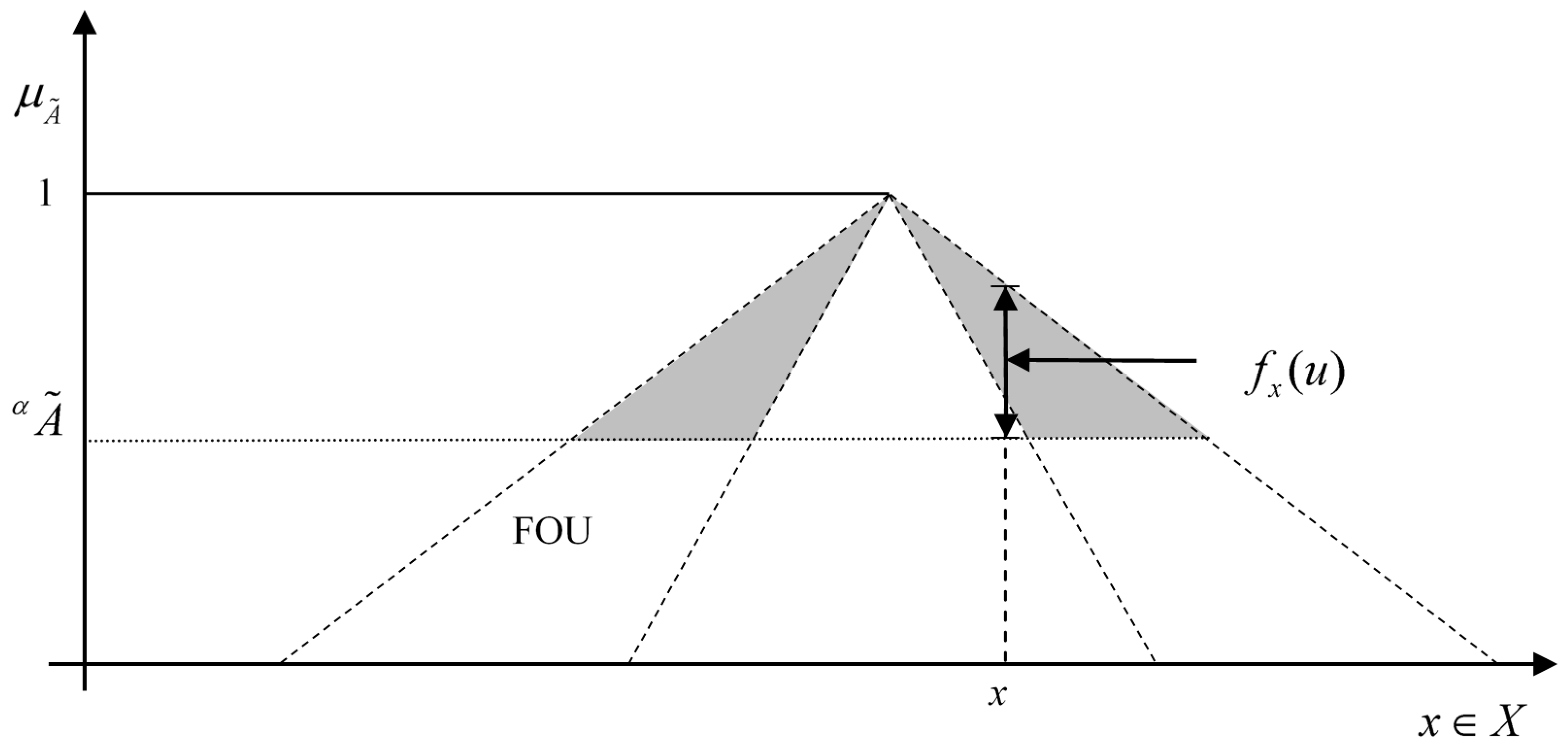
Definition 1.

A T2FS$\tilde{A}$(as shown Figure 1) in the universe of discourse X can be represented by a type-2 membership function${\mu }_{\tilde{A}}$[22] as follows:

$$\tilde{A}={\displaystyle {\int }_{x\in X}{\displaystyle {\int }_{u\in J_X}{\mu }_{\tilde{A}}\left(x,u\right)/\left(x,u\right)}}$$

(1)

where$J_X$denotes an interval in [0, 1], and${\displaystyle \iint }$denotes the union over all admissible x and u. The LMF denotes the lower membership function of T2FS; the UMF represents the upper membership function of T2FS. Fuzzy sets can be represented through α-cuts (also known as α level), which basically are horizontal slices over its membership function. The α-cut of A is defined as${}^{\alpha }\tilde{A}=\left\{x|{\mu }_{\tilde{A}}x\ge \alpha \right\}$. f (x) represents the secondary membership function of T2FSs. This approach simplifies the computation of any function f (x) in presence of fuzzy sets. Figure 2 shows a particular value over${}^{\alpha }\tilde{A}$for α = 0.6.

The concept of footprint of uncertainty (FOU) of an interval Type-2 fuzzy set (IT2FS) can be extended to α-planes [23], which are represented by a T2FS through α-planes that are z-slices over the secondary membership $f_x(u)/u$. An α-plane for a general T2FS $\tilde{A}$, denoted as ${\tilde{A}}_{\alpha }$, is the union of all primary memberships of $\tilde{A}$ whose secondary grades are greater than or equal to α, ($0\le \alpha \le 1$), i.e.,

$${\tilde{A}}_{\alpha }=\underset{x\in X}{\cup }\left\{\left(x,u\right)|{\mu }_{\tilde{A}}\left(x,u\right)\ge \alpha \right\},$$

(2a)

$${\tilde{A}}_{\alpha }={\displaystyle \underset{x\in X}{\cup }{S}_{\tilde{A}}\left(x|\alpha \right)},$$

(2b)

$$S_{\tilde{A}}\left(x|\alpha \right)={\left({\mu }_{\tilde{A}}\left(x\right)\right)}_{\alpha }.$$

(2c)

To reduce the uncertainty of fuzzy coefficients, Figuroa [24] presented a method of T2FSs that is based on the existing α-cuts and α-planes algorithm.

Definition 2.

Let${}^{\alpha }\tilde{A}$be the α-cut, and${\tilde{A}}_{\alpha }$be the α-plane of$\tilde{A}$. Denoting${\alpha }_c=c$and${\alpha }_p=p$, the$\alpha =\left\{c,p\right\}$representation of$\tilde{A}$, namely,${}^{c,p}\tilde{A}$, is the union of all${\alpha }_c$and${\alpha }_p$of$\tilde{A}$:

$${}^{c,p}\tilde{A}={\displaystyle \underset{x\in X}{\cup }{\displaystyle \underset{u\in J_x}{\cup }\left\{\left(x,u\right)|{\mu }_{\tilde{A}}\left(x,u\right)\ge \left\{c,p\right\}\right\}}},$$

(3a)

$${}^{c,p}\tilde{A}={\displaystyle \underset{x\in X}{\cup }{S}_{\tilde{A}}\left(x|c,p\right)},$$

(3b)

$$S_{\tilde{A}}\left(x|c,p\right)={}^{c,p}\left({\mu }_{\tilde{A}}\left(x\right)\right).$$

(3c)

This definition combines both the α-cut and the α-plane of $\tilde{A}$ into a single representation. This definition is also useful to examine the effect of decomposing $\tilde{A}$ into slices, and it can be useful for computing functions of fuzzy sets via a fuzzy extension principle. Thus, any Type-2 fuzzy set A can be recomposed using ${}^{c,p}\tilde{A}$, as defined as follows. This part given the definition of representation algorithm.

Definition 3.

Let${}^{\alpha }\tilde{A}$be the α-cut and${\tilde{A}}_{\alpha }$be the α-plane of A. Thus, the fuzzy set$\tilde{A}$can be composed as the union of all${\alpha }_c$and${\alpha }_p$:

$$\tilde{A}={\displaystyle \underset{{\alpha }_c\in \left[0,1\right]}{\cup }{\displaystyle \underset{{\alpha }_p\in \left[0,1\right]}{\cup }\left\{c,p\right\}}}$$

(4)

Definition 4.

Let${}^{\alpha }\tilde{A}$be the α-cut and${\tilde{A}}_{\alpha }$be the α-plane of$\tilde{A}$. The boundaries of${}^{\alpha }\tilde{A}$given${\tilde{A}}_{\alpha }$, namely${}^{c,p}\tilde{A}^L$and${}^{c,p}\tilde{A}^R$, are defined as:

$${}^{c,p}\tilde{A}^L=\left[\underset{x}{\inf }{}^{c,p}\overline{\mu }_{\tilde{A}}\left(a,u\right);\underset{x}{\inf }{}^{c,p}\underset{\_}{\mu }_{\tilde{A}}\left(a,u\right)\right]=\left[{}^{c,p}\tilde{A}^{L+},{}^{c,p}\tilde{A}^{L-}\right],$$

(5a)

$${}^{c,p}\tilde{A}^R=\left[\underset{x}{\inf }{}^{c,p}\underset{\_}{\mu }_{\tilde{A}}\left(a,u\right);\underset{x}{\inf }{}^{c,p}\overline{\mu }_{\tilde{A}}\left(a,u\right)\right]=\left[{}^{c,p}\tilde{A}^{R-},{}^{c,p}\tilde{A}^{R+}\right],$$

(5b)

That is,

$${}^{c,p}\tilde{A}=\left[\left[{}^{c,p}\tilde{A}^{L+},{}^{c,p}\tilde{A}^{L-}\right],\left[{}^{c,p}\tilde{A}^{R-},{}^{c,p}\tilde{A}^{R+}\right]\right].$$

(5c)

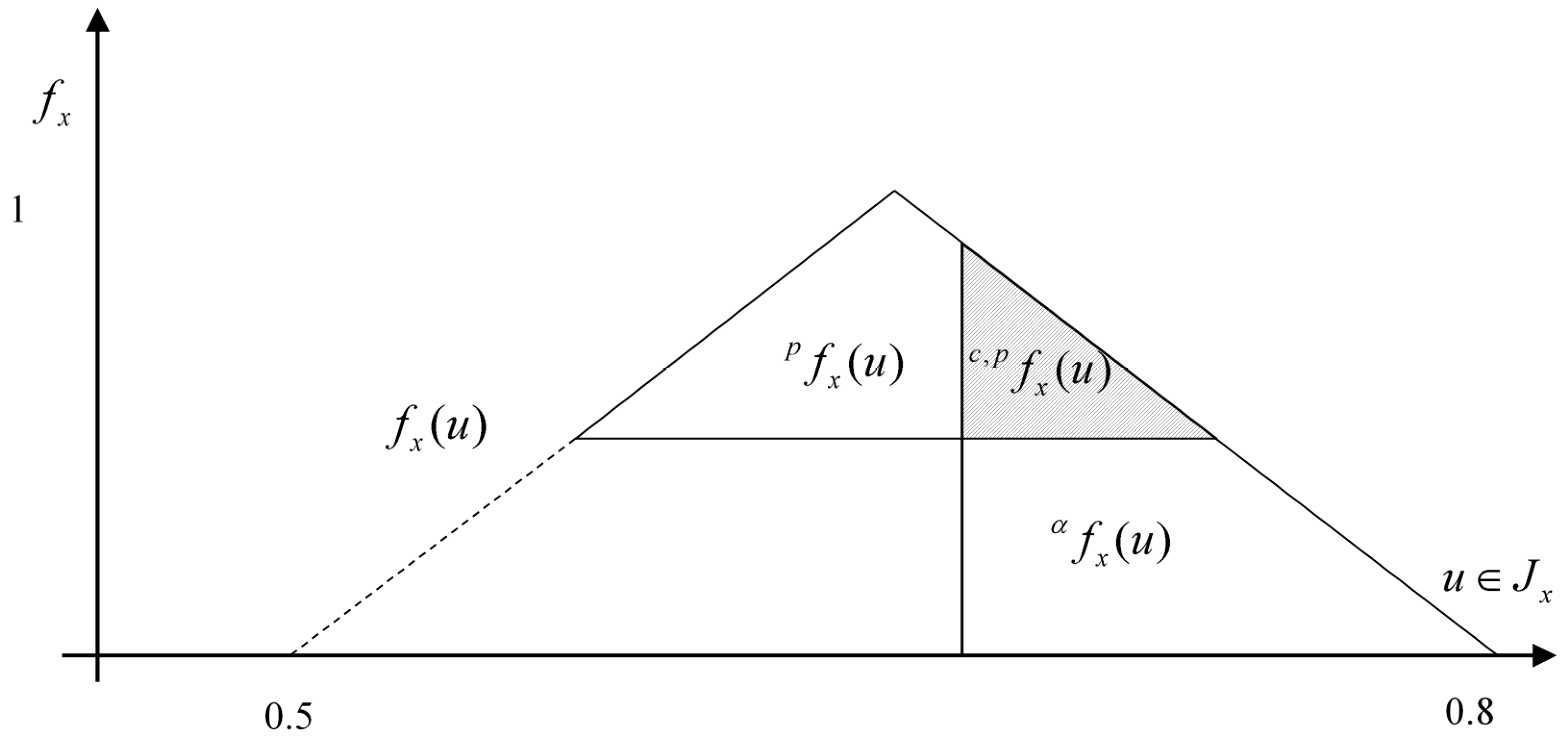
The above definition given the solution of representation algorithm, In Figure 3, the larger solid triangle in the right side shows a vertical slice of X where ${}^{\alpha }\tilde{A}$ cuts $f_x\left(u\right)$ over α = 0.6. Moreover, the ${}^p\tilde{A}$ for the p-cut value of ${}^p{f}_x\left(u\right)$ (p = 0.5) is shown as the solid triangle at the top of Figure 3.

The solutions from the above equations can be combined into ${}^{c,p}\tilde{A}$ for $\left\{c,p\right\}=\left\{0.6,0.5\right\}$ over a particular $x\in X$, leading to ${}^{0.6,0.5}\tilde{A}$, as shown in Figure 3. Consequently, the intersection of all $x\in X$ for $\left\{c,p\right\}=\left\{0.6,0.5\right\}$ is organized as ${}^{c,p}\tilde{A}$ over c = 0.6, p = 0.5, as shown in the shadow part of Figure 3. According to the figure, this double cut produces a small uncertainty area, i.e., a larger c, p of the cut corresponds to less uncertainty.

Thus, according to the inexact linear programming (ILP) [25], the T2FS programming model can be rewritten, as follows:

$$\mathrm{Min}{f}^{\pm }=C^{\pm }{X}^{\pm }$$

(6a)

subject to

$$A^{\pm }{X}^{\pm }\tilde{\le }\underset{˜}{\tilde{B}}$$

(6b)

$$X^{\pm }\ge 0$$

(6c)

where $A^{\pm }$ and $C^{\pm }$ represent interval parameters, $A^{\pm }\in R^{\pm \left(m\times n\right)}$ and $C^{\pm }\in {\left\{R^{\pm }\right\}}^{1\times n}$, respectively, and $\underset{˜}{\tilde{B}}\in {\underset{˜}{\tilde{b}}}^{\left(m\times 1\right)}$ where $\tilde{b}$ is a T2FSs coefficient.

According to the arithmetic operations on the T2FS coefficients introduced above, a α-representation level $\left\{c,p\right\}$ is selected for all T2FS coefficients. Thus, model (6) can be rewritten as:

$$\mathrm{Max}{f}^{\pm }=C^{\pm }{X}^{\pm }$$

(7a)

subject to

$$A^{\pm }{X}^{\pm }\tilde{\le }\left[\left[{}^{c,p}\tilde{B}^{L+},{}^{c,p}\tilde{B}^{L-}\right],\left[{}^{c,p}\tilde{B}^{R-},{}^{c,p}\tilde{B}^{R+}\right]\right],$$

(7b)

$$X^{\pm }\ge 0.$$

(7c)

To solve model (7), it can be transferred into two boundary models by using a robust two-step-method (RTSM), as follows:

$$\mathrm{Max}{f}^{\pm }=C^{\pm }{X}^{\pm }$$

(8a)

subject to

$$A^{\pm }{X}^{\pm }\le \left[{}^{c,p}\tilde{B}^{L+},{}^{c,p}\tilde{B}^{L-}\right],$$

(8b)

$$X^{\pm }\ge 0,$$

(8c)

and

$$\mathrm{Max}{f}^{\pm }=C^{\pm }{X}^{\pm }$$

(9a)

subject to

$$A^{\pm }{X}^{\pm }\le \left[{}^{c,p}\tilde{B}^{R-},{}^{c,p}\tilde{B}^{R+}\right],$$

(9b)

$$X^{\pm }\ge 0.$$

(9c)

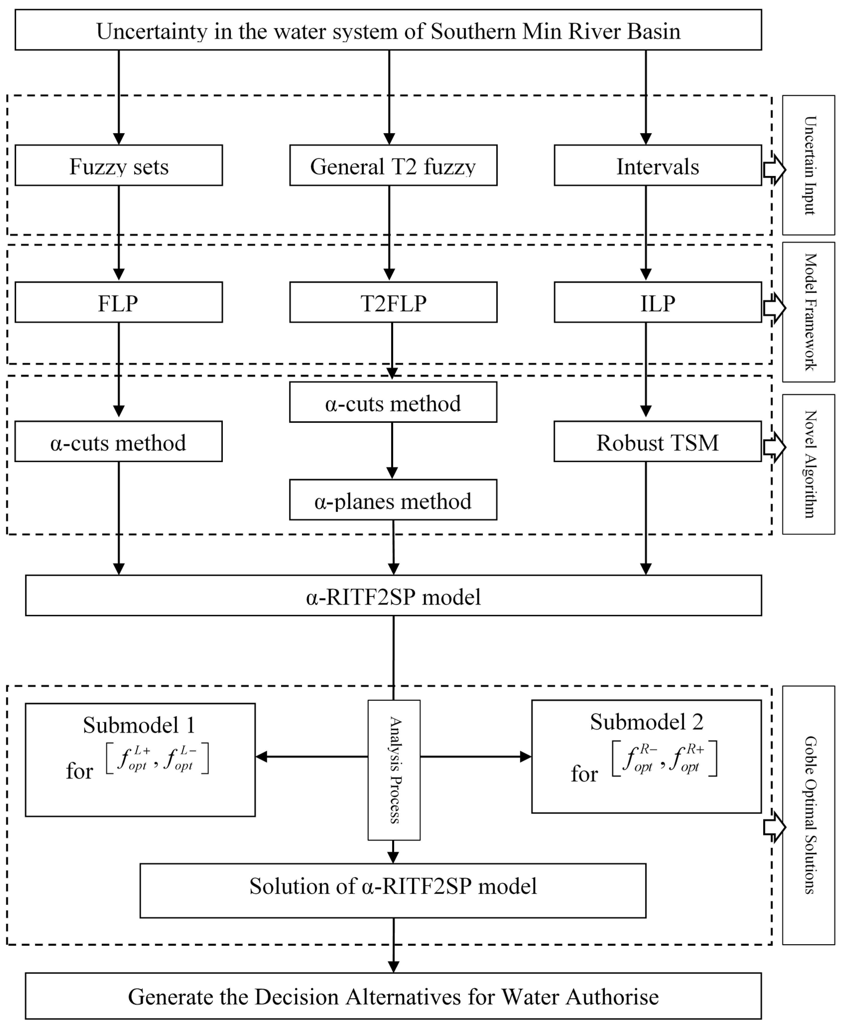
According to Chinneck and Ramadan [26], we convert each boundary model into two LP models corresponding to upper and lower approximation intervals. Thus, the optimal solutions for model (6) are as follows (Figure 4 shows the relevant flow chart of the proposed approach from a linear programming perspective).

$$f^{\pm }=\left[\left[f_{opt}^{L+},f_{opt}^{L-}\right]\left[f_{opt}^{R-},f_{opt}^{R+}\right]\right],$$

(10a)

$$x^{\pm }=\left[\left[x_{opt}^{L+},x_{opt}^{L-}\right]\left[x_{opt}^{R-},x_{opt}^{R+}\right]\right].$$

(10b)

Briefly, the procedure for solving the α-RITF2SP approach can be summarized, as follows:

Step 1 

Formulate the inexact linear programming T2 model.

Step 2 

Apply the α-cuts and α-planes methods over the higher degrees of uncertainty.

Step 3 

Obtain two more specific inexact LP submodels.

Step 4 

Solve these two T2FSsLP functions by applying the RTSM algorithm.

Step 5 

Obtain the optimal solutions $x_{jopt}^{R\&L*}$ and $f_{opt}^{R\&L*}$.

3. Water Resources Management under Uncertainty

3.1. Overview of the Water System

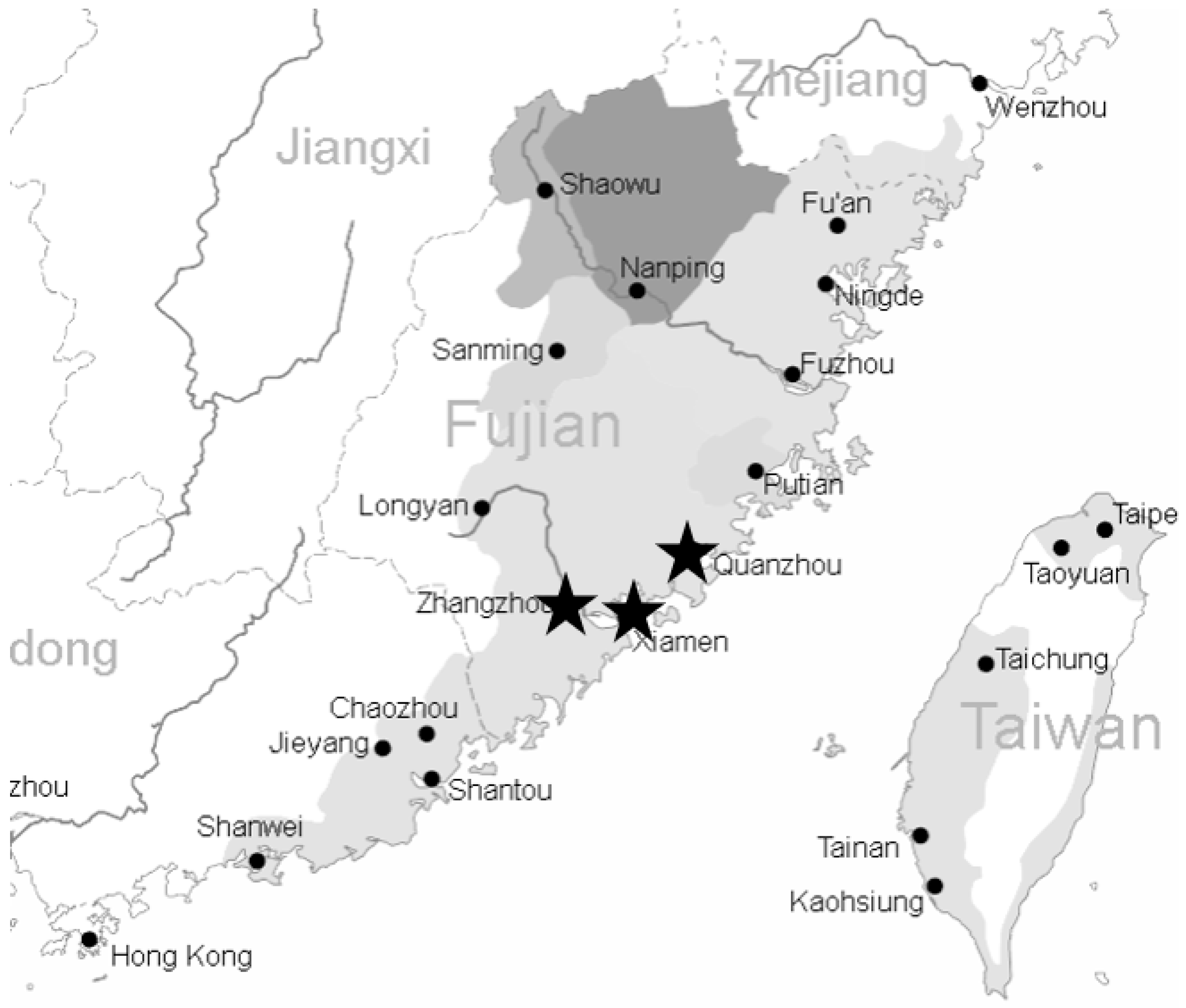
The developed model is applied to a real case study of water resources management for the agriculture area. Figure 5 (the picture was obtained from wikimedia.org) [27] shows the location map of the southern Min River basin. The river basin is located in the South Asian subtropics; the area mainly refers to the areas of Xiamen, Zhangzhou, and Quanzhou, including the Jiulong River. The river basin has superior climatic conditions, adequate light and heat resources, fertile land, and abundant products. In the southern Min agricultural basin, there are more than five million people, and the land accounts for 13% of the province. Although the southern Min River basin has superior climatic conditions, natural disasters occur frequently because of the unstable monsoon climate. Although adequate light and heat resources are favorable conditions for agricultural development, these conditions have not been fully utilized. The spatial and temporal distributions of rainfall are uneven, making this basin vulnerable to natural disasters, such as floods and droughts. These phenomena provide the most basic information on the status of water resources in the region.

This river basin has a variety of landforms, such as plains, hills, mesas, basins, and mountains. These geomorphological features are conducive to the comprehensive development of agriculture. However, the per capita arable land is small, at only 0.8 acres. This arable land area is less than the average (1.5 acres) and it is even lower than the world’s per capita arable land area (4.7 acres). Moreover, most of the land resources available for cultivation have been used; this situation restricts the development of crop farming to some extent. However, the water treatment cost of arable land has not been considered in this model due to the currently local environmental and agricultural regulations.

Because of its advantageous geographical location, adequate resources, and a strong rainforest landscape, this natural environment is suitable for a variety of living creatures. Rich biological resources have created excellent conditions for agriculture, animal husbandry, forestry, fishery, and other industries. However, these conditions have not been effectively and reasonably used and developed; in addition, many rare wild animal resources, forest resources, and various economic fish resources have been destroyed to varying degrees, resulting in low efficiency, and the ecological environment has also been destroyed. The water resources in the southern Min River basin are relatively abundant, but the current utilization rate is low and thus has great development potential in a model of planning patter. In addition to considering water supply in Xiamen and other places, it is also possible to consider the rational planning and construction of hydroelectric power stations.

The water basin has a long history and pleasant scenery; this situation has created rich tourism resources in this area. For example, in Xiamen City, with its strong subtropical climate, graceful and clean city bay style, passionate and simple overseas Chinese customs, delicious tropical fruits, and fresh seafood products, is a nationally famous tourist city, attracting tourists from all over the country. The large number of tourists visiting Xiamen has exerted great pressure on its water supply, water use, water treatment, and garbage disposal as an increase in the cost of water treatment.

3.2. Analysis of the Environmental Issues of Southern Min Area

3.2.1. Ecological Issues

Floods are an historical problem in this watershed. As a result of typhoons, rainstorms, climate change, and soil erosion, flood disasters are frequent. The causes of more serious soil erosion are as follows: (1) overexploitation of orchards and tea plantation, and (2) overexploitation of mines and rivers and planting inappropriate trees in large areas, destroying vegetation on the ground. The increasing severity of soil erosion has also contributed to the occurrence of floods. As a result, a vicious cycle has been formed. Ecological problems can reduce the ability of natural water bodies to degrade pollutions, thereby increasing the cost of water treatment for this region.

3.2.2. Air Pollution Issues

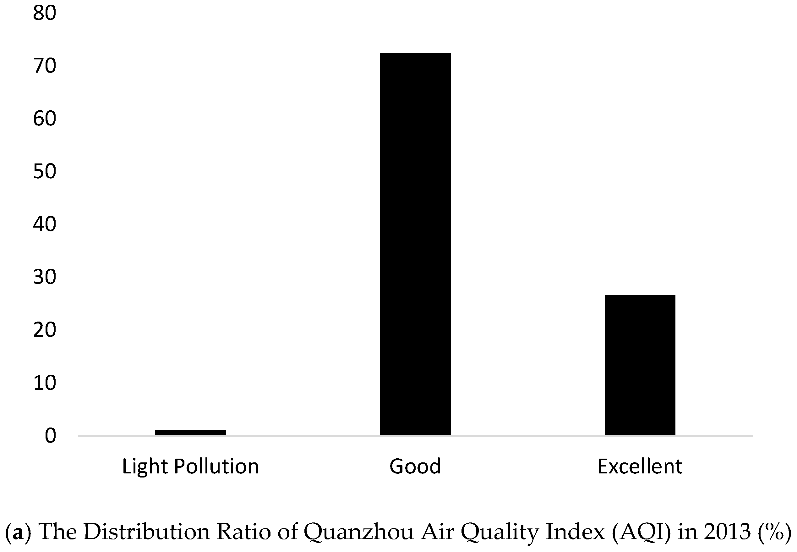
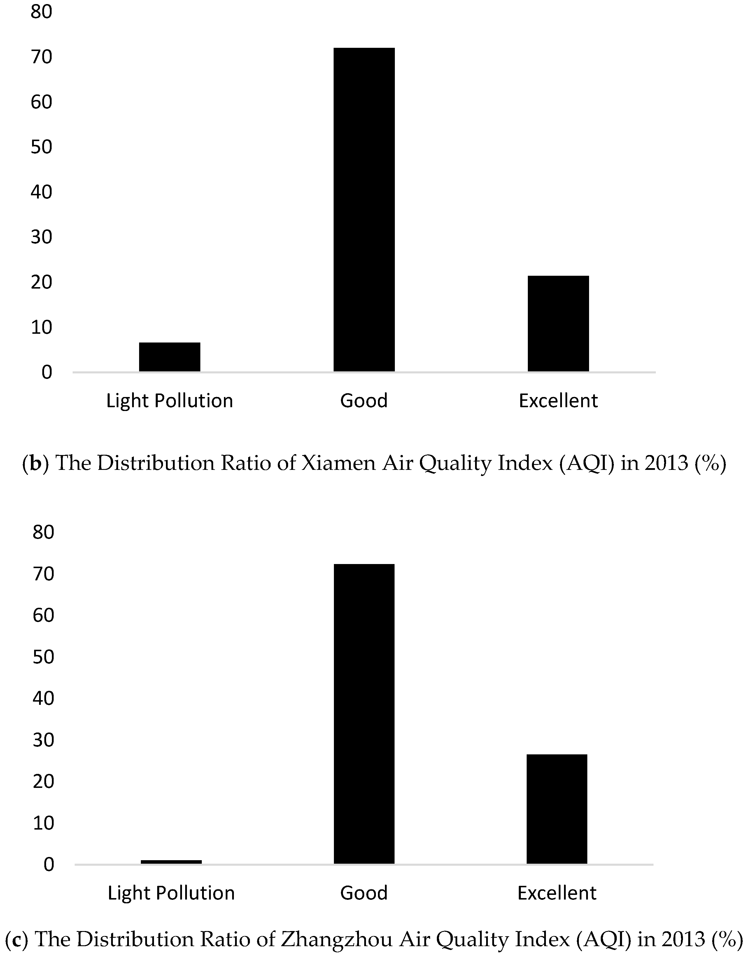
There is a strong correlation between atmospheric deposition and water quality. But, the air pollution in the southern Min River basin is much better than that in many other cities of China. Figure 6 represents the air quality of index for this area. However, many problems have been raised in recent years. The severe air pollution has caught the attention of the regional environmental protection office. Recently, Xiamen City has taken some measures to improve air quality of the city, such as strengthening the treatment of exhaust pollution from motor vehicles, the control of fume pollution in the catering industry, and the prevention of dust. In contrast, for the cities of Quanzhou and Zhangzhou, the supervision and control requirements must be strengthened in the future. The issues of air pollution among cities should be redefined and monitored more clearly. Thus, this strengthening will improve water quality and reduce water treatment costs.

3.2.3. Water Pollution Issues

The excessive and unsustainable construction of hydropower stations led to the drought and low flow conditions in the tributaries and main stream of the Jiulong River. “Lake servitization” increases the hydraulic retention time and easily leads to water bloom and water eutrophication in the reservoir area. In 2009, there were algal bloom incidents in the area of the North-Stream Reservoir that caused the pollution of drinking water in Xiamen City, severely affecting daily lives. This example represents just one of the causes of water pollution; the author believes that the main reason may be the discharges of various pollution sources of wastewater. As a result, overall reasonable planning of the construction of hydropower stations should be implemented to amplify the advantages and reduce the disasters that are caused by the hydropower stations.

Because eighty percent of Xiamen’s drinking water comes from the Jiulong River, the pollution of Jiulong River is an extremely important issue. Affected by industries such as the Longyan Paper Mill and the Zhangzhou Sugar Mill, the north-stream and west-stream of Jiulong River have suffered from various levels of pollution. However, in the wet season, the water flow is large and the dilution effect is more obvious; as a result, the water quality of the watershed will be better than that in the dry season. Therefore, a summary of the water pollutants in the area is as follows: (1) the pollution that is caused by the breeding of livestock and poultry from upstream of this river. There is a large amount of pig breeding in the basin, with most of the farms experiencing serious pollution problems, and their treatment facilities are incomplete, with some farms even directly discharging the wastewater into the river. As a result, the nitrogen, phosphorus, and other indicators in the relevant water areas and land in the basin have been seriously exceeded. (2) The construction of the hydropower station is unreasonable, with the distribution density being excessively high, thereby preventing the natural purification of water quality to proceed normally. As a result, the water resources are prone to algae blooms and eutrophication. (3) Although the discharge amounts from the industries (such as paper mills, sugar factories, pharmaceutical factories, and metal processing plants) were not very high, the pollutants from these plants accounted for more than 90% of the watershed. These companies must rectify the situation, as economic conditions permit, and minimize the total amount of pollution. Excessive usages of chemical fertilizers and pesticides also pollute nearby waters resources and land to a certain extent, thereby directly or indirectly endangering the cities welfare. (4) The quantity and scale of wastewater and waste treatment facilities do not meet the corresponding needs in this area.

Table 1. The annual pollutant discharges of the Fujian Province in 2013.

Proportion of Total Discharges (%)	Industrial Source	Agricultural Source	Municipal Source	Treatment Facility	Traffic Vehicle
COD	12.70	32.56	54.09	0.65	--
NH3-N	6.76	35.23	57.57	0.44	--
SO2	94.75	--	5.25
NOX	75.43	--	0.54	0.01	24.03

and

Table 2. Pollutant discharges from the agricultural source of the Fujian province in 2013.

Proportions of Total Discharges (%)	Livestock and Poultry Farming	Aquaculture Industry	Planting Industry
COD	84.22	15.78	--
NH3-N	66.10	21.80	12.10
SO2	59.12	11.67	29.21
NOX	60.70	15.42	23.88

show the pollution discharges from the sources. Therefore, in this rapid economic development, if decision makers want to develop and maintain a green economy or/and recycling economy, the environmental protection facilities, policies, and regulations should also develop rapidly to match the pace of social and economic developments.

3.3. Modeling Formulation

The maximum profit of the water resources system is inevitably guided by the industries that make reasonable usage of water resources. However, these industries will discharge waste water and therefore generate corresponding treatment costs. Consequently, the maximum profit should be received under a reasonable manufacturing process. The largest profit is equal to the net profit minus both the water cost and the cost of treatment of pollution. However, the manufacturing process must satisfy every constraint: the total amount of water usages should not exceed the carrying capacity of the local environmental resources; the total amount of sewage treatment should remain within the capacity of the wastewater treatment plants; the industrial scale constraint on production should consider the economic factors and equipment constraints for every industry; and, the expenditure of investments cannot exceed the government budget. It is also obvious that the water system must be profitable; thus, all input values are considered to be nonnegative. In this study, the planning horizon covers 15 years with five years per period, i.e., 2018–2022, 2022–2027, and 2027–2032. During the planning horizon, Fujian will upgrade its industrial structure. However, limited by water resource, the size of population will be controlled strictly. According to the future economic and social development of Fujian, and considering uncertain events, the forecasted water demand for each end-user is uncertain with three possible scenarios, i.e., low, medium and high, with the corresponding probability of 0.25, 0.6, and 0.15, respectively. Therefore, the α-RITF2SP model can be formulated, as follows:

$$\mathrm{Max}{f}^{\pm }=f_1^{\pm }-f_2^{\pm }-f_3^{\pm }-f_4^{\pm }-f_5^{\pm }$$

(1)

Water utilization benefits

$$f_1^{\pm }={\displaystyle \sum _{s=1}^3{p}_s{\displaystyle \sum _{t=1}^3\left({\displaystyle \sum _{h=1}^{2}NB{P}_{th}^{\pm }}\cdot P{T}_{sth}^{\pm }+{\displaystyle \sum _{i=1}^{2}NB{M}_{ti}^{\pm }}\cdot M{T}_{sti}^{\pm }+{\displaystyle \sum _{j=1}^{9}NB{F}_{tj}^{\pm }}\cdot F{T}_{stj}^{\pm }+NB{E}_t^{\pm }\cdot E{T}_{st}^{\pm }+NB{I}_t^{\pm }\cdot I{T}_{st}^{\pm }\right)}}$$

(11a)

(2)

Water supply cost

$$f_2^{\pm }={\displaystyle \sum _{t=1}^3{\displaystyle \sum _{m=1}^{5}WS{C}_{tm}^{\pm }}}\left({\displaystyle \sum _{h=1}^{2}P{W}_{tmh}^{\pm }}+{\displaystyle \sum _{i=1}^{2}M{W}_{tmi}^{\pm }}+{\displaystyle \sum _{j=1}^{9}F{W}_{tmj}^{\pm }}+E{W}_{tm}^{\pm }+I{W}_{tm}^{\pm }\right)$$

(3)

Extra water supply cost

$$f_3^{\pm }={\displaystyle \sum _{t=1}^3{\displaystyle \sum _{m=4}^5{\displaystyle \sum _{s=1}^3{p}_s\cdot EWS{C}_{tm}^{\pm }\left({\displaystyle \sum _{s=1}^{3}EP{W}_{tmhs}^{\pm }}+{\displaystyle \sum _{i=1}^{2}EM{W}_{tmis}^{\pm }}+{\displaystyle \sum _{j=1}^{9}EF{W}_{tmjs}^{\pm }}+EE{W}_{tms}^{\pm }+EI{W}_{tms}^{\pm }\right)}}}$$

(4)

Sewage treatment cost

$$f_4^{\pm }={\displaystyle \sum _{t=1}^3{\displaystyle \sum _{s=1}^3{p}_s\cdot {\gamma }_t^{\pm }\cdot {\eta }_t^{\pm }}}\left({\displaystyle \sum _{h=1}^{2}TC{P}_{th}^{\pm }}\cdot P{T}_{sth}^{\pm }+{\displaystyle \sum _{i=1}^{2}TC{M}_{ti}^{\pm }}\cdot M{T}_{sti}^{\pm }+{\displaystyle \sum _{j=1}^{9}TC{F}_{tj}^{\pm }}\cdot F{T}_{stj}^{\pm }+TC{E}_t^{\pm }\cdot E{T}_{st}^{\pm }+TC{I}_t^{\pm }\cdot I{T}_{st}^{\pm }\right)$$

(5)

Water shortage penalty

$$f_5^{\pm }={\displaystyle \sum _{t=1}^3{\displaystyle \sum _{s=1}^3{p}_s\cdot \left\{\begin{array}{l}{\displaystyle \sum _{h=1}^{2}CP{P}_{th}^{\pm }}\cdot \left(P{D}_{sth}^{\pm }-P{T}_{sth}^{\pm }\right)+{\displaystyle \sum _{i=1}^{2}CP{M}_{ti}^{\pm }}\cdot \left(M{D}_{sti}^{\pm }-M{T}_{sti}^{\pm }\right)+\\ {\displaystyle \sum _{j=1}^{9}CP{F}_{tj}^{\pm }}\cdot \left(F{D}_{stj}^{\pm }-F{T}_{stj}^{\pm }\right)+CP{E}_t^{\pm }\cdot \left(E{D}_{st}^{\pm }-E{T}_{st}^{\pm }\right)+CP{I}_t^{\pm }\cdot \left(I{D}_{st}^{\pm }-I{T}_{st}^{\pm }\right)\end{array}\right\}}}$$

Constraints:

(1)

Water availability constraints:

$$\begin{array}{l}\left({\displaystyle \sum _{h=1}^{2}P{W}_{tmh}^{\pm }}+{\displaystyle \sum _{i=1}^{2}M{W}_{tmi}^{\pm }}+{\displaystyle \sum _{j=1}^{9}F{W}_{tmj}^{\pm }}+E{W}_{tm}^{\pm }+I{W}_{tm}^{\pm }\right)+\\ \left({\displaystyle \sum _{h=1}^{2}EP{W}_{tmhs}^{\pm }}+{\displaystyle \sum _{i=1}^{2}EM{W}_{tmis}^{\pm }}+{\displaystyle \sum _{j=1}^{9}EF{W}_{tmjs}^{\pm }}+EE{W}_{tms}^{\pm }+EI{W}_{tms}^{\pm }\right)\le \otimes A{W}_{tm\max }^{\pm },\forall t,s,m=1,2,3\end{array}$$

(11b)

(2)

Seawater desalinization constraints:

$$\begin{array}{l}\left({\displaystyle \sum _{h=1}^{2}P{W}_{tmh}^{\pm }}+{\displaystyle \sum _{i=1}^{2}M{W}_{tmi}^{\pm }}+{\displaystyle \sum _{j=1}^{9}F{W}_{tmj}^{\pm }}+E{W}_{tm}^{\pm }+I{W}_{tm}^{\pm }\right)+\\ \left({\displaystyle \sum _{h=1}^{2}EP{W}_{tmhs}^{\pm }}+{\displaystyle \sum _{i=1}^{2}EM{W}_{tmis}^{\pm }}+{\displaystyle \sum _{j=1}^{9}EF{W}_{tmjs}^{\pm }}+EE{W}_{tms}^{\pm }+EI{W}_{tms}^{\pm }\right)\le AD{D}_t^{\pm }\cdot {\mu }_t^{\pm }\cdot D{C}_t^{\pm },\forall t,s,m=4\end{array}$$

(11c)

(3)

Water recycling constraints:

$$\begin{array}{l}\left({\displaystyle \sum _{h=1}^{2}P{W}_{tmh}^{\pm }}+{\displaystyle \sum _{i=1}^{2}M{W}_{tmi}^{\pm }}+{\displaystyle \sum _{j=1}^{9}F{W}_{tmj}^{\pm }}+E{W}_{tm}^{\pm }+I{W}_{tm}^{\pm }\right)+\\ \left({\displaystyle \sum _{h=1}^{2}EP{W}_{tmhs}^{\pm }}+{\displaystyle \sum _{i=1}^{2}EM{W}_{tmis}^{\pm }}+{\displaystyle \sum _{j=1}^{9}EF{W}_{tmjs}^{\pm }}+EE{W}_{tms}^{\pm }+EI{W}_{tms}^{\pm }\right)\\ \le {\alpha }_t^{\pm }\cdot {\lambda }_t^{\pm }\cdot {\eta }_t^{\pm }\cdot \left({\displaystyle \sum _{h=1}^{2}P{T}_{sth}^{\pm }}+{\displaystyle \sum _{i=1}^{2}M{T}_{sti}^{\pm }}+{\displaystyle \sum _{j=1}^{9}F{T}_{stj}^{\pm }}+E{T}_{st}^{\pm }+I{T}_{st}^{\pm }\right),\forall t,s,m=5\end{array}$$

(11d)

(4)

Water supply and demand balance constraints:

$${\displaystyle \sum _{m=1}^5\left(P{W}_{tmh}^{\pm }+EP{W}_{tmhs}^{\pm }\right)}\cdot \left(1-{\beta }_{tm}^{\pm }\right)=P{T}_{sth}^{\pm },\forall t,s,h$$

(11e)

$${\displaystyle \sum _{m=1}^5\left(M{W}_{tmi}^{\pm }+EM{W}_{tmis}^{\pm }\right)}\cdot \left(1-{\beta }_{tm}^{\pm }\right)=M{T}_{sti}^{\pm },\forall t,s,i$$

(11f)

$${\displaystyle \sum _{m=1}^5\left(F{W}_{tmj}^{\pm }+EF{W}_{tmjs}^{\pm }\right)}\cdot \left(1-{\beta }_{tm}^{\pm }\right)=F{T}_{stj}^{\pm },\forall t,s,j$$

(11g)

$${\displaystyle \sum _{m=1}^5\left(E{W}_{tm}^{\pm }+EE{W}_{tms}^{\pm }\right)}\cdot \left(1-{\beta }_{tm}^{\pm }\right)=E{T}_{st}^{\pm },\forall t,s$$

(11h)

$${\displaystyle \sum _{m=1}^5\left(I{W}_{tm}^{\pm }+EI{W}_{tms}^{\pm }\right)}\cdot \left(1-{\beta }_{tm}^{\pm }\right)=I{T}_{st}^{\pm },\forall t,s$$

(11i)

$$P{D}_{sth}^{\pm }-P{T}_{sth}^{\pm }\le e_t^{\pm }\cdot P{D}_{sth}^{\pm },\forall s,t,h$$

(11j)

$$M{D}_{sth}^{\pm }-M{T}_{sth}^{\pm }\le e_t^{\pm }\cdot M{D}_{sth}^{\pm },\forall s,t$$

(11k)

$$F{D}_{sti}^{\pm }-F{T}_{sti}^{\pm }\le e_t^{\pm }\cdot F{D}_{sti}^{\pm },\forall s,t,i$$

(11l)

$$E{D}_{st}^{\pm }-E{T}_{st}^{\pm }\le e_t^{\pm }\cdot E{D}_{st}^{\pm },\forall s,t$$

(11m)

$$I{D}_{st}^{\pm }-I{T}_{st}^{\pm }\le e_t^{\pm }\cdot I{D}_{st}^{\pm },\forall s,t$$

(11n)

(5)

Nonnegative constraints:

$$P{W}_{tmh}^{\pm }\ge 0,EP{W}_{tmhs}^{\pm }\ge 0\forall t,m,h,s$$

(11o)

$$M{W}_{tmi}^{\pm }\ge 0,EM{W}_{tmis}^{\pm }\ge 0\forall t,m,i,s$$

(11p)

$$F{W}_{tmj}^{\pm }\ge 0,EF{W}_{tmjs}^{\pm }\ge 0,\forall t,m,j,s$$

(11q)

$$E{W}_{tm}^{\pm }\ge 0,EE{W}_{tms}^{\pm }\ge 0,\forall t,m,s$$

(11r)

$$I{W}_{tm}^{\pm }\ge 0,EI{W}_{tms}^{\pm }\ge 0,\forall t,m,s$$

(11s)

where the index of model (11) is given as follows:

$f^{\pm }$	total system profit;
t	the period;
h	petrochemical industry, h = 1, 2 for different companies;
i	marine chemical industry, h = 1, 2 for different companies;
j	fine chemical industry, j = 1, ..., 9 for different companies;
m	water source, m = 1, 2, 3, 4, 5 for surface water, underground water, transferred water, desalination water and reused water, respectively;
s	water level;
$\otimes$	T2 fuzzy set;
$p_s$	scenario probability;
$NB{P}_{th}^{\pm }$	water utilization benefit from petrochemical industry h in period t (million ¥/106 m3);
$NB{M}_{ti}^{\pm }$	water utilization benefit from marine chemical industry i in period t (million ¥/106 m3);
$NB{F}_{tj}^{\pm }$	water utilization benefit from fine chemical industry j in period t (million ¥/106 m3);
$NB{E}_t^{\pm }$	water utilization benefit from energy industry in period t (million ¥/106 m3);
$NB{I}_t^{\pm }$	water utilization benefit from steel industry in period t (million ¥/106 m3);
$P{T}_{ths}^{\pm }$	water consumed by petrochemical industry h in period t under scenario s (106 m3);
$M{T}_{tis}^{\pm }$	water consumed by marine chemical industry i in period t under scenario s (106 m3);
$F{T}_{tjs}^{\pm }$	water consumed by fine chemical industry j in period t under scenario s (106 m3);
$E{T}_{ts}^{\pm }$	water consumed by energy industry in period t under scenario s (106 m3);
$I{T}_{ts}^{\pm }$	water consumed by steel industry in period t under scenario s (106 m3);
$WS{C}_{ti}^{\pm }$	water supply cost from source m in period t (million ¥/106 m3);
$EWS{C}_{ti}^{\pm }$	extra cost from water source m in period t (million ¥/106 m3);
$P{W}_{tmh}^{\pm }$	provided amount from water source m to petrochemical industry h in period t (106 m3);
$M{W}_{tmi}^{\pm }$	provided amount from water source m to marine chemical industry i in period t (106 m3);
$F{W}_{tmj}^{\pm }$	provided amount from water source m to fine chemical industry j in period t (106 m3);
$E{W}_{tm}^{\pm }$	provided amount from water source m to energy industry in period t (106 m3);
$I{W}_{tm}^{\pm }$	provided amount from water source m to steel industry in period t (106 m3);
$EP{W}_{tmhs}^{\pm }$	extra supply from water source m to petrochemical industry h under scenario s in period t (106 m3);
$EM{W}_{tmis}^{\pm }$	extra supply from water source m to marine chemical industry i under scenario s in period t (106 m3);
$EF{W}_{tmjs}^{\pm }$	extra supply from water source m to fine chemical industry j under scenario s in period t (106 m3);
$EE{W}_{tms}^{\pm }$	extra supply from water source m to energy industry under scenario s in period t (106 m3);
$EI{W}_{tms}^{\pm }$	extra supply from water source m to steel industry under scenario s in period t (106 m3);
${\gamma }_t^{\pm }$	discharge ratio of wastewater per unit water consumption j during period t;
${\eta }_t^{\pm }$	sewage treatment ratio of emission from during period t;
$TC{P}_{th}^{\pm }$	sewage treatment cost for petrochemical industry h in period t (million ¥/106 m3);
$TC{M}_{ti}^{\pm }$	sewage treatment cost for marine chemical industry i in period t (million ¥/106 m3);
$TC{F}_{tj}^{\pm }$	sewage treatment cost for fine chemical industry j in period t (million ¥/106 m3);
$TC{E}_t^{\pm }$	sewage treatment cost for energy industry in period t (million ¥/106 m3);
$TC{I}_t^{\pm }$	sewage treatment cost for steel industry in period t (million ¥/106 m3);
$CP{P}_{th}^{\pm }$	penalty cost for water shortage for petrochemical industry h in period t (million ¥/106 m3);
$CP{M}_{ti}^{\pm }$	penalty cost for water shortage for marine chemical industry i in period t (million ¥/106 m3);
$CP{F}_{tj}^{\pm }$	penalty cost for water shortage for fine chemical industry j in period t (million ¥/106 m3);
$CP{E}_t^{\pm }$	penalty cost for water shortage for energy industry in period t (million ¥/106 m3);
$CP{I}_t^{\pm }$	penalty cost for water shortage for steel industry in period t (million ¥/106 m3);
$P{D}_{ths}^{\pm }$	water demand for petrochemical industry h during period t under scenario s (106 m3);
$M{D}_{tis}^{\pm }$	water demand for marine chemical industry i during period t under scenario s (106 m3);
$F{D}_{tjs}^{\pm }$	water demand for fine chemical industry j during period t under scenario s (106 m3);
$E{D}_{ts}^{\pm }$	water demand for energy industry during period t under scenario s (106 m3);
$I{D}_{ts}^{\pm }$	water demand for steel industry during period t under scenario s (106 m3);
$A{W}_{ti\max }^{\pm }$	maximum available water (106 m3);
$AD{D}_t^{\pm }$	average working days (days/year);
${\mu }_t^{\pm }$	production efficiency;
$D{C}_t^{\pm }$	the capacity of sea water desalinization (106 m3/day);
${\alpha }_t^{\pm }$	recycling ratio during period t;
${\beta }_t^{\pm }$	transmission loss ratio during period t; and,
$e_t^{\pm }$	maximum tolerance of water shortage during period t.

3.4. Data Source

Combing the specific circumstances of the southern Min River basin, the enterprises or factories that must be analyzed and optimized are divided into petrochemicals, marine chemicals, fine chemicals, energy utilization industry, and steel industry. Taking into account the current study of the southern Min River basin, this paper focused on the major pollution sources as the objects of modeling that are typically represented in the three cities of Xiamen, Zhangzhou, and Quanzhou. However, because of the changes of the industries, these data do not represent the entire industries but represent only part of them.

Table 3. Planed water consumption (10⁶ m³).

Industry Category	t = 1			t = 2			t = 3
	Low	Medium	High	Low	Medium	High	Low	Medium	High
Petrochemical industry
h = 1	[20.5, 20.9]	[20.7, 21.1]	[20.9, 21.3]	[21.5, 21.9]	[21.7, 22.1]	[21.9, 22.3]	[22.5, 22.9]	[22.7, 23.1]	[22.9, 23.3]
h = 2	[20.1, 20.6]	[20.3, 20.8]	[20.5, 21.0]	[21.1, 21.6]	[21.3, 21.8]	[22.1, 22.5]	[22.1, 22.6]	[22.3, 22.8]	[23.1, 23.5]
Marine chemical industry
i = 1	[3.3, 3.5]	[3.5, 3.7]	[3.7, 3.9]	[4.3, 4.5]	[4.5, 4.7]	[4.7, 4.9]	[5.3, 5.5]	[5.5, 5.7]	[5.7, 5.9]
i = 2	[2.6, 3.1]	[2.8, 3.3]	[3.0, 3.5]	[3.6, 4.1]	[3.8, 4.3]	[4.0, 4.5]	[4.6, 5.1]	[4.8, 5.3]	[5.0, 5.5]
Fine chemical industry
j = 1	[7.5, 8.2]	[7.7, 8.4]	[7.9, 8.6]	[8.5, 9.2]	[8.7, 9.4]	[8.9, 9.6]	[9.5, 10.2]	[9.7, 10.4]	[9.9, 10.6]
j = 2	[7.1, 7.8]	[7.3, 8.0]	[7.5, 8.2]	[8.1, 8.8]	[8.5, 9.0]	[8.5, 9.2]	[9.1, 10.8]	[9.3, 10.0]	[9.5, 10.2]
j = 3	[7.3, 8.2]	[7.5, 8.4]	[7.7, 8.6]	[8.5, 9.2]	[8.7, 9.4]	[8.7, 9.6]	[9.3, 10.2]	[9.5, 10.4]	[9.7, 10.6]
j = 4	[7.3, 8.5]	[7.5, 8.7]	[7.7, 8.9]	[8.3, 9.5]	[8.7, 9.7]	[8.7, 9.9]	[9.3, 10.5]	[9.5, 10.7]	[9.7, 10.9]
j = 5	[6.5, 7.6]	[6.7, 7.8]	[6.9, 8.0]	[8.5, 8.6]	[8.7, 8.8]	[7.9, 9.0]	[8.5, 9.6]	[8.7, 9.8]	[8.9, 10.0]
j = 6	[6.8, 7.1]	[7.0, 7.3]	[7.2, 7.5]	[8.5, 8.1]	[8.9, 9.0]	[8.2, 8.5]	[8.8, 9.1]	[9.0, 9.3]	[9.2, 9.5]
j = 7	[6.6, 6.9]	[6.8, 7.1]	[7.0, 7.3]	[7.7, 7.9]	[8, 8.1]	[8.0, 8.3]	[8.6, 8.9]	[8.8, 9.1]	[9.0, 9.3]
j = 8	[7.2, 7.9]	[7.4, 8.1]	[7.6, 8.3]	[8.0, 8.9]	[8.6, 9.1]	[8.6, 9.3]	[9.2, 9.9]	[9.4, 10.1]	[9.6, 10.3]
j = 9	[6.1, 7.2]	[6.3, 7.4]	[6.5, 7.6]	[8.6, 8.2]	[7.5, 8.4]	[7.5, 8.6]	[8.1, 9.2]	[8.3, 9.4]	[8.5, 9.6]
Energy industry	[41.6, 42.5]	[41.8, 42.8]	[42.0, 43.1]	[42.6, 43.5]	[4.28, 43.8]	[43.0, 44.1]	[43.6, 4.45]	[4.38, 44.8]	[44.0, 45.1]
Steel industry	[53.2, 54.6]	[54.5, 54.8]	[54.8, 55.0]	[54.2, 55.6]	[54.5, 55.8]	[54.8, 56.0]	[55.2, 56.6]	[55.5, 56.8]	[55.8, 57.0]

and

Table 4. The economic parameters (10⁴ CNY/m³).

Industry Category	Net Benefit for Water Utilization			Penalty Cost for Water Shortage
	t = 1	t = 2	t = 3	t = 1	t = 2	t = 3
Petrochemical industry
h = 1	[10.5, 11]	[12.2, 13.0]	[13.1, 14.3]	[11.5, 12.5]	[14.5, 16.8]	[16.5, 19.2]
h = 2	[10.5, 11]	[12.2, 13.0]	[13.1, 14.3]	[11.5, 12.5]	[14.5, 16.8]	[16.5, 19.2]
Marine chemical industry
i = 1	[2.8, 3.0]	[3.5, 3.8]	[4.2, 4.9]	[4.0, 5.0]	[4.8, 5.5]	[5.0, 6.0]
i = 2	[2.8, 3.0]	[3.5, 3.8]	[4.2, 4.9]	[4.0, 5.0]	[4.8, 5.5]	[5.0, 6.0]
Fine chemical industry
j = 1	[22.5, 23.5]	[23.5, 24.5]	[24.6, 25.8]	[23.5, 25.5]	[24.5, 26.5]	[26.5, 28.5]
j = 2	[22.5, 23.5]	[23.5, 24.5]	[24.6, 25.8]	[23.5, 25.5]	[24.5, 26.5]	[26.5, 28.5]
j = 3	[22.5, 23.5]	[23.5, 24.5]	[24.6, 25.8]	[23.5, 25.5]	[24.5, 26.5]	[26.5, 28.5]
j = 4	[22.5, 23.5]	[23.5, 24.5]	[24.6, 25.8]	[23.5, 25.5]	[24.5, 26.5]	[26.5, 28.5]
j = 5	[22.5, 23.5]	[23.5, 24.5]	[24.6, 25.8]	[23.5, 25.5]	[24.5, 26.5]	[26.5, 28.5]
j = 6	[22.5, 23.5]	[23.5, 24.5]	[24.6, 25.8]	[23.5, 25.5]	[24.5, 26.5]	[26.5, 28.5]
j = 7	[22.5, 23.5]	[23.5, 24.5]	[24.6, 25.8]	[23.5, 25.5]	[24.5, 26.5]	[26.5, 28.5]
j = 8	[22.5, 23.5]	[23.5, 24.5]	[24.6, 25.8]	[23.5, 25.5]	[24.5, 26.5]	[26.5, 28.5]
j = 9	[22.5, 23.5]	[23.5, 24.5]	[24.6, 25.8]	[23.5, 25.5]	[24.5, 26.5]	[26.5, 28.5]
Energy industry	[11.5, 12.0]	[13.2, 14.0]	[14.3, 14.8]	[12.5, 14.5]	[14.5, 16.5]	[16.5, 18.5]
Steel industry	[4.8, 5.0]	[5.5, 5.8]	[6.1, 6.8]	[5.0, 6.0]	[6.5, 7.5]	[7.0, 8.0]

list the parameter data from the relevant area obtained from the Environmental Status Bulletin of Fujian Province [28] and the Statistical Bulletin and the local market price in 2013 that are required for the model calculations [29]. By considering that there are too many small chemical companies in this area to consider, in this study, we selected only nine of them to represent this chemical industry. In the future, if more data can be found, all of the chemical companies should be considered. The data show the approximate price range of the respective products of the companies or factories in various industries in each term. The uncertain changes in prices are affected by many factors, such as demand relations, seasonal changes, international market prices, and domestic policy implications.

4. Results Analysis

4.1. System Benefit through the Water Model

Figure 7 shows the water benefits under different ratios of wastewater treatment through the α-RITF2SP model. Clearly, a higher wastewater treatment rate will bring a higher profit to this area, rather causing a loss of system benefit, as some people think. With the η coefficient of processing from 0.1 to1.0, this water system’s profit has increased six-fold, both at a higher system cost and lower system cost. This system profit indicates that, if the water manager reduces the wastewater treatment rate, then it will directly affect the net profit of the local area. Moreover, according to current wastewater treatment rate (92%), the total system benefit would be from 51,143.97 × 10⁴ yuan to 52,596.09 × 10⁴ yuan, corresponding to the cost between upper bound and lower bound. This result implies that increased wastewater treatment rate in next five years would result in higher profits of the water resources system.

4.2. Water Planning Results

Table 5. Optimal water supply allocation in different periods (10⁶ m³).

Industry Category	t = 1					t = 2					t = 3
	m = 1	m = 2	m = 3	m = 4	m = 5	m = 1	m = 2	m = 3	m = 4	m = 5	m = 1	m = 2	m = 3	m = 4	m = 5
Petrochemical industry
h = 1	[0.0, 0.34]	0.34	17.26	0	0	0	[0.3, 0.7]	0	18.1	0	0.17	0.34	[18.8, 19.14]	0	0
h = 2	[0.0, 0.17]	0.34	[0.0, 0.43]	16.91	0	[0.0, 0.3]	18.1	0	0	0	[0.0, 0.86]	18.97	0	0	[0.0, 0.26]
Marine chemical industry
i = 1	[0.0, 0.37]	2.83	0	0	0	[0.2, 0.3]	[0.3, 3.4]	3.4	0	0	0.34	0	0	[4.2, 4.38]	0
i = 2	0	[2.23, 2.83]	[0.0, 0.43]	0	0	[0.3, 0.4]	[0.3, 2.8]	2.8	0	0	[0.0, 0.43]	3.95	0	0	0
Fine chemical industry
j = 1	[0.0, 2.58]	[4.86, 6.78]	0	0	0	[0.0, 17.4]	0.5	0	0	[3.2, 29.4]	[0.0, 0.86]	1.2	[0.0, 7.73]	0	[0.0, 7.3]
j = 2	[0.0, 7.04]	0	0	[0.0, 38]	0	[0.0, 7.9]	0	0	0	[0.0, 7.8]	[0.0, 9.27]	0	0	[0.0, 8.15]	0
j = 3	[0.0, 7.38]	[0.0, 6.61]	0	0	0	0	[0.0, 10.9]	0	0	[0.0, 8.2]	0	[0.0, 0.17]	0	[0.0, 39.41]	[9.1, 34.47]
j = 4	0	0	[4.98, 6.61]	[0.0, 2.66]	0	0	0	[8.0, 27.8]	0	0	[31.52, 52.3]	[2.91, 2.92]	0	[0.0, 61.82]	[0.0, 8.59]
j = 5	0	[0.0, 5.92]	0	0	[0.0, 6.87]	0	[0.0, 7.7]	[0.0, 7.3]	0	0	0	0	[0.0, 34.7]	0	0
j = 6	[0.0, 6.1]	[0.17, 6.19]	0	0	0	[7.6, 7.7]	0	0	0	0	[0.34, 1.2]	[6.61, 7.56]	0	[0.0, 0.6]	0
j = 7	[0.0, 6.27]	0	0	[0.0, 6.01]	0	[0.0, 33.9]	0	0	[7.1, 33.7]	[0.0, 28.4]	0	0	[0.0, 7.98]	[0.0, 7.73]	0
j = 8	[9.79, 39.5]	[0.01, 0.51]	0	0	0	[0.0, 0.9]	[0.0, 0.2]	[7.6, 20.1]	0	0	0	0	[0.0, 18.64]	0	[0.0, 8.24]
j = 9	0	[0.0, 20.35]	0	[0.0, 29.72]	[297.2, 304.07]	[0.0, 7.4]	0	0	0	[0.0, 7.00]	[0.0, 8.24]	0	0	[0.0, 7.3]	0
Energy industry	0	1.72	[0.0, 0.77]	0	34	0	[1.7, 2.6]	[0.0, 34.3]	[0.0, 34.2]	0	[0.0, 0.86]	[13.58, 13.66]	0	[22, 48]	0
Steel industry	0	1.71	15.63	[28.33, 29.53]	0	0	[0.9, 1.7]	0	0	45.93	0	[0.86, 1.72]	0	0	46.2

represents the results received through the α-RITF2SP model for the southern Min River basin (10⁶ m³). The index m indicates the five different water sources received individually from surface water, underground water, transferred water, desalination water, and reused water. For example, in period 1, which was the first five year period, the major water resources for the first petrochemical industry was 17.26 × 10⁶ m³ supported from the transferred water; the second petrochemical industry was 16.91 × 10⁶ m³ received from the desalination water. Moreover, the first marine chemical industry should obtain 2.83 × 10⁶ m³ water from the underground water; the second of the marine chemical industry also should obtain 2.23 to 2.83 × 10⁶ m³ water from the underground water. In the southern Min area, nine fine chemical industry companies were selected for the water resources planning. Because the operation costs of each company are different and the amount of water required is different, the resources of water supply are not the same. Consequently, through the results of the study model, the main source of water management shows that the first company should receive 4.86 to 6.78 × 10⁶ m³ from the underground water resource; the second company should receive 7.04 × 10⁶ m³ from the surface water resource; the third one should receive 7.38 × 10⁶ m³ from the surface water resources and 6.61 × 10⁶ m³ from the underground water resource; when index j is equal to 4, the major source of this company would be 6.61 × 10⁶ m³ from the transferred water; the major sources of the fifth company are 6.87 × 10⁶ m³ of underground water and 5.92 × 10⁶ m³ of reused water; and, the sixth company can obtain 6.1 × 10⁶ m³ and 6.19 × 10⁶ m³ from surface water and underground water, respectively; the last three fine chemical industry companies should receive 6.27 × 10⁶ m³, 39.5 × 10⁶ m³ and 304.7 × 10⁶ m³ from the surface water and reused water sources. Furthermore, the energy industry should use 34 × 10⁶ m³ from reused water; the steel industry should utilize 28.33 to 29.53 × 10⁶ m³ of desalination water. For the last two industries with high water consumption and high cost, increasing the utilization rate of reclaim water is a better method to solve the water resources shortage than purchasing water from other sources. In periods 2 and 3, the water supply remained in a similar situation to that of period 1. As implied from above solutions, if the water manager seeks to pursue higher system profit, then it is necessary to utilize these reclaimed water sources, including desalination water and recycled water. Figure 8 shows the ratio of fresh water to reclaimed water in three different periods. The fresh water includes surface water, underground water, and transferred water sources.

4.3. Discussion

From the above analysis, the results can be in the form of interval numbers, which highlight the difference between higher profit and lower profit. The differences associated with the water limited supply or shortages reflect different uncertainties. For example, the costs of policy requirements or optimistic circumstances correspond to the upper boundary of high benefit. Conversely, if the costs are below the critical policy requirements, then the lower boundary of low profit can be generated to support the decision makers. Moreover, some irrational factors, either man-made or natural, also reduce the profits of water systems. The uncontrollable typhoon season of the southern Min area comes with substantial rainfall, which might be used to supply the urban water demand. Furthermore, the reliability of the water treatment facilities and water supply equipment as well as the management model of local company both reduce the net profit of the water resources systems. However, these factors may cause additional water purchases from other cities or areas with a relative higher cost.

Table 6. Extra water supply for scenario 1 (10⁶ m³).

Industry Category	Period 1					Period 2					Period 3
	m = 1	m = 2	m = 3	m = 4	m = 5	m = 1	m = 2	m = 3	m = 4	m = 5	m = 1	m = 2	m = 3	m = 4	m = 5
Petrochemical industry
h = 1	0	0	0	0	0	0	0.17	0	0	0	0	0.34	0	0	0
h = 2	0	0	0	0	0	0	0.17	0	0	0	[0, 0.17]	0.34	0	0	0
Marine chemical industry
i = 1	0	[0, 0.17]	0	0	0	[0, 0.37]	[0.17, 0.34]	0	0	0	0	0.34	0	0	0
i = 2	0	0	0	0	0	0	0.17	0	0	0	0	0.34	0	0	0
Fine chemical industry
j = 1	0	4.8	0	0	0	0	2.4	0	0	0	0	0	0	0	0
j = 2	0	0	0	0	0	0	0	0	0	0	0	0	0	0	0
j = 3	0	0	0	0	0	0	0	0	0	0	0	0	0	0	0
j = 4	0	0	0	0	0	0	0	0	0	0	0	0	0	0	0
j = 5	0	0	0	0	0	0	0	0	0	0	0	0	0	0	0
j = 6	[0, 0.55]	0	0	0	0	0	0	0	0	0	[0, 0.37]	[0, 0.17]	0	0	0
j = 7	0	0	0	0	0	0	0	0	0	0	0	0	0	0	0
j = 8	0	0.51	0	0	0	0	[0, 0.51]	0	0	0	0		0	0	0
j = 9	0	0	0	0	0	0	0	0	0	0	0	0	0	0	0
Energy industry	0	[0, 0.28]	0	0	0	0	0.86	0	0	0	0	1.72	0	0	0
Steel industry	0	0	0	0	0	0	0.86	0	0	0	0	1.72	0	0	0

,

Table 7. Extra water supply for scenario 2 (10⁶ m³).

Industry Category	Period 1					Period 2					Period 3
	m = 1	m = 2	m = 3	m = 4	m = 5	m = 1	m = 2	m = 3	m = 4	m = 5	m = 1	m = 2	m = 3	m = 4	m = 5
Petrochemical industry
h = 1	0	0	0	0	0	0	0.17	0	0	0	0	[0, 0.34]	0	0	0
h = 2	0	0	0	0	0	0	0.17	0	0	0	0	[0, 0.86]	0	0	0
Marine chemical industry
i = 1	0	0	0	0	0	[0, 0.17]	0.17	0	0	0	[0, 0.34]	0.34	0	0	0
i = 2	0	0	0	0	0	[0, 0.14]	0.17	0	0	0	[0, 0.34]	0.34	0	0	0
Fine chemical industry
j = 1	0	4.46	0	0	0	0	2.92	0	0	0	0	0	0	0	0
j = 2	0	0	0	0	0	0	0	0	0	0	0	0	0	0	0
j = 3	0	0	0	0	0	0	0	0	0	0	0	0	0	0	0
j = 4	0	0	0	0	0	0	0	0	0	0	0	0	0	0	0
j = 5	0	[0, 0.57]	0	0	0	0	0	0	0	0	0	0	0	0	0
j = 6	0	0	0	0	0	0	0	0	0	0	0	0	0	0	0
j = 7	0	0	0	0	0	0	0	0	0	0	0	0	0	0	0
j = 8	[0, 0.86]	[0, 0.2]	0	0	0	0	0	0	0	0	[0, 0.86]	0	0	0	0
j = 9	0	0	0	0	0	0	0	0	0	0	0	0	0	0	0
Energy industry	0	0	0	0	0	0	0.86	0	0	0	0	[0.86, 1.72]	0	0	0
Steel industry	0	0	0	0	0	0	0.86	0	0	0	0	1.72	0	0	0

and

Table 8. Extra water supply for scenario 3 (10⁶ m³).

Industry Category	Period 1					Period 2					Period 3
	m = 1	m = 2	m = 3	m = 4	m = 5	m = 1	m = 2	m = 3	m = 4	m = 5	m = 1	m = 2	m = 3	m = 4	m = 5
Petrochemical industry
h = 1	[0, 0.1]	0	0	0	0	[0, 0.17]	0	0	0	0	[0, 0.1]	[0, 0.34]	0	0	0
h = 2	[0, 0.85]	0	0	0	0	[0, 0.86]	0.17	0	0	0	0	0.86	0	0	0
Marine chemical industry
i = 1	0	0	0	0	0	[0, 0.17]	0	0	0	0	[0, 0.34]	0	0	0	0
i = 2	0	0	0	0	0	0	0.17	0	0	0	[0, 0.34]	0.34	0	0	0
Fine chemical industry
j = 1	0	1.2	0	0	0	0	0	0	0	0	[0, 0.86]	0	0	0	0
j = 2	0	0	0	0	0	0	0	0	0	0	0	0	0	0	0
j = 3	0	[0, 0.17]	0	0	0	0	0	0	0	0	0	[0, 0.17]	0	0	0
j = 4	0	2.92	0	0	0	0	2.92	0	0	0	0	0	0	0	0
j = 5	0	0	0	0	0	0	0	0	0	0	0	0	0	0	0
j = 6	[0.34, 1.2]	0	0	0	0	0	0	0	0	0	0	0	0	0	0
j = 7	0	0	0	0	0	0	0	0	0	0	0	0	0	0	0
j = 8	0	0	0	0	0	0	0	0	0	0	0	0	0	0	0
j = 9	0	0	0	0	0	0	0	0	0	0	0	0	0	0	0
Energy industry	0	0	0	0	0	[0, 0.85]	0	0	0	0	0	0.86	0	0	0
Steel industry	0	0	0	0	0	0	0.86	0	0	0	0	1.72	0	0	0

indicate the extra water supply for every industry under different scenarios. Scenarios 1, 2, and 3 represented three cases of high, medium, and low water supply, respectively, as described above. In lower water level season, petrochemical industry needs 0.17 × 10⁶ m³ extra water supply from other imported underground water during period 2. This is because the cost of water treatment is already higher than the price of water in the field. This is also the reason of a lack of underground water that is caused by special coastal features. During the period 3, petrochemical industries 0.17 × 10⁶ m³ and 0.34 × 10⁶ m³ extra water to support the scarcity in both surface water and underground water. It also confirms the lack of water resources, including the reused water in this region.

Figure 9 shows the additional water purchases from other cities or areas. The figure presents the amount of extra water supply for all industries, including the petrochemical industry, marine chemical industry, fine chemical industry, energy industry, and steel industry, under different scenarios. As shown in Figure 9, over the three periods, the fine chemical industry is the primary water purchaser. For example, in period 1 and period 2 under scenario 1, this industry requires 5.86 × 10⁶ m³ water, with 2.91 × 10⁶ m³ obtained from additional water supplies from other sources. This type of industry is not suitable for using reclaimed water, thereby increasing the cost of its production. The usage of reclaimed water can only be used within certain types of industries, some of which may not suitable in the southern Min River basin. Under scenario 2, the marine chemical industry should purchase 6.09 × 10⁶ m³, 0.65 × 10⁶ m³, and 1.36 × 10⁶ m³ for period 1, period 2, and period 3, respectively. In addition, under scenario 3, the companies of the chemical industry in this area should also purchase extra water to obtain high system benefit.

In general, the results indicate that a normal fuzzy set linear programming method is insufficiently enough to reflect uncertain information in the decision-making process. The simplification of membership function can cause unreliable or even confusing decision processes. This is the reason that higher economic coefficients but a lower profit of the water system management. This system characteristic will lead to an unreliable decision on water recourses planning. Therefore, the developed method displays a more capable solution and it can deal with the higher levels of uncertainty due to the fuzzy membership. Thus, the α-RITF2SP model is more increased in uncertainty evaluation, as well as it improves the system reliability of water resources and pollution control. As a result, a more suitable planning of a diversity of water resources is the necessary condition to achieve maximum profitability of the water resource system. Thus, the α-RITF2SP model here is a good tool to support decision making for the water authorities in this region.

5. Conclusions

Through integrating the advantages of both α-cuts and α-plane into the interval optimal framework, an α-representation of the inexact T2 fuzzy sets programming method (α-RITF2SP) was developed. The α-RITF2SP is based on interval programming, and Type-2 fuzzy sets linear programming under uncertainty. The method addresses the higher level uncertainty in function constraints to obtain more accurate results than other fuzzy linear programming models. The method uses the α-plane to solve the problems in the third dimension of uncertainty; these problems are expressed as T2FSs in the function. The inexact linear programming is useful to indicate the fluctuation of environmental resources and data changes after the uncertain events occur to accurately determine the water system uncertainty.

The proposed method was applied to the real case study of the southern Min River basin water resources management system. The α-RITF2SP provided water authorities with input under experts’ perceptions or linguistic uncertainty with the following advantages: (1) the α-represent method, which can effectively implement membership function uncertainty into the optimization process, is an alternative perspective to indicate the general T2FSs; (2) the method obtains a more specific representation of a T2FS, while α-cuts have been well used among classical fuzzy sets and α-planes also have been well utilized for T2FSs; (3) both the input uncertainty and linguistic uncertainty are solved through two different cuts and planes, in which the α-cuts approach is desirable for the decision makers, whereas the α-planes approach is desirable in constrained water resources; (4) the developed method is applied to a practical issue in the Southern Min River basin; and, (5) it provides the desired water resources management plans with maximum system benefit under limited natural resources to the decision makers of this area.

The α-RITF2SP approach was introduced for the first time in this study to the optimization field of water resources management. This approach enables an extended application of linear programming of T2FSs to other resources and environmental management problems based on the fields of interest of researchers.