Interactive Tuning Tool of Proportional-Integral Controllers for First Order Plus Time Delay Processes

Abstract

Engineering education and, particularly, control engineering, has shown growth in research and development activities during last years. Currently, proportional–integral (PI) and proportional–integral–derivative (PID) controllers are the most commonly used in industrial process applications. Nonetheless, it is reported that many of them are badly tuned. From an educational perspective, it is crucial for the student to understand the importance of tuning a control loop correctly. This paper presents an interactive tool focused on the study of PI controllers. The tool provides a set of tuning rules for both open-loop stable and unstable first order plus time delay processes. The different tuning rules can be compared interactively by the user, allowing a critical analysis of basic concepts about stability, robustness, and performance in PI control loops. In addition to educational purposes, the tool has been developed, taking into account practical considerations, such as simulation with a controller discrete implementation, process input saturations, and windup effect. We evaluated students’ achievement in the final examination in the Automatic Control course of the Electronics Engineering degree. Students showed significant improvement in their understanding of PI controller design. A survey and a practical case study were performed to evaluate the effectiveness of the proposed tool.

1. Introduction

1.1. Background

Proportional–integral (PI) and proportional–integral–derivative (PID) controllers are most commonly used in industrial processes, owing to their satisfactory control effect, acceptable robustness, and simple control structure [1]. According to [2], it is estimated that over 90% of control loops employ PID controllers and, on many occasions, with the derivative gain set to zero (i.e., PI control). By and large, PI and PID have been the classic type of controllers since mid-20th century, and they continue as the most often used control scheme [3]. As it was concluded at the International Federation of Automatic Control Conference on Advances in PID control in 2012, PID/PI controllers will remain as the main implemented control algorithms, in spite of other promising proposals, such as model predictive control paradigms [4]. However, as shown in several surveys, there is a lack of engagement between the industrial world and the academic community. For instance, according to [5], 68% of PID/PI controllers are poorly tuned, and have an unacceptable performance. Consequently, it is necessary to progress in the education and training of these kinds of controllers.

1.2. Formulation of the Problem of Interest for This Investigation

Several works have been written on the tuning of PID/PI controllers [6,7]. Using tuning rules is the most direct way to set up controller parameters [6]. Many of these rules are based on a simple model of process dynamics and, in particular, the widely adopted plant model is the first order plus time delay (FOPTD) [3,8]. In addition, several developed PI tuning rules are based on the FOPTD model. For these reasons and, also considering that PI controllers are most common in industry [9], the control problem, studied in this work, is defined as follows: the plant model is a FOPTD process given by (1), where K represents the stationary gain, T the time constant, and τ the time delay of the process. The PI controller is given by (2), where K_P represents the proportional gain and K_I the integral gain (thus, the integral time constant T_I equals K_P/K_I).

$$G\left(s\right)=\frac{K}{Ts+1}{e}^{-\tau ·s}$$

(1)

$$C\left(s\right)=K_P+\frac{K_I}{s}$$

(2)

Tuning a control loop can be defined as the adjustment of its control parameters (K_P and K_I in the case of a PI controller) to the optimum values for a desired control response. One of the main objectives of this work is to analytically determine the set of K_P–K_I values for which the closed-loop system is stable. For this purpose, and for the analysis of the control response given specific K_P and K_I values, the feedback control system of Figure 1 is assumed. The controlled variable is given by y, sp represents the reference signal, u symbolizes the control signal, and load the input disturbance.

1.3. Literature Survey

Since the PID controller tuning rules of Ziegler and Nichols (1942) [10], different and new approaches have been developed, mainly concerned with feedback controllers tuned either for a well-damped fast response to a step change in the controller set-point, or emphasizing the importance of disturbance rejection in the design [11]. Some of the developed methods considered only the system performance, by using an integrated error criteria (Integral Absolute Error (IAE), Integral Square Error (ISE) or Integral Time Absolute Error (ITAE)) as, for example, the pioneering methodologies developed by Murrill et al. (1967) [12] or Rovira et al. (1969) [13], or the more recent work by Awouda and Mamat (2010) [14]. Conversely, other developed tuning rules consider mainly the robustness, such as AMIGO (Approximate M constrained Integral Gain Optimization) developed by Åström and Hägglund [15,16], or those developed by Ho et al. [17]. Another relevant research line is the set of tuning rules that proposes a tradeoff between performance and robustness, or between servo and regulation modes [11,18]. There are also tuning rules specifically developed for unstable FOPTD processes, ranging from relatively simple analytic tuning formulae [19] to more complex techniques using evolutionary or heuristic algorithms [20,21]. Nevertheless, as mentioned before, a great majority of tuning rules is based on FOPTD models [7,22], and there are extensions to other structures, such as the second order plus dead time (SOPDT), the integrator plus dead time (IPDT), and the first order and integrator plus dead time (FOIDT). The number of developed tuning rules based on the FOPTD model is large compared with the proposals that exist for second order systems [23]. Several of the aforementioned tuning rules and others are collected in O’Dwyer’s work [6]. However, it is important to note the lack of comparative analysis with respect to the robustness and performance of closed-loop systems compensated with the associated controllers. As noted in [5], one of the gaps in existing research in the area is a critical analysis of available tuning rules, rather than the proposal of new tuning rules.

1.4. Scope and Contribution of This Study

Most of the relevant automatic control concepts, such as time and frequency responses, stability and robustness analysis, root locus, lag-lead compensation, PID controller design, and so on, have a nice intuitive graphical representation. These representations have been accepted for years as an excellent way to introduce automatic control concepts that are difficult to understand for the students. Computers have excellent graphical features for representing most of these relevant control concepts easily. Integrated development environments, such as MATLAB, Scilab, LabVIEW, Sysquake, or Easy Java Simulations, can help to create graphical and interactive applications, reducing development time and programming. Graphical visualization and interactive tools can contribute to accelerating the learning process, making traditional lectures more attractive and interesting [24,25]. Specifically, interactivity is considered a powerful tool, providing a bidirectional information flow that creates an active learning experience. Considering this aspect, interactive tools for teaching control are supported by several advantages [26,27,28,29,30]: (a) learning efficiency is improved by using computer aided design and analysis tools; (b) instantaneous observation of the corresponding effects when modifying properties facilitates the learning processes; (c) they support the combination between theory and practice contents; (d) the interactive comparison of different tuning rules allows to understand fundamental ideas about performance, robustness and stability in PI control loops.

This work presents an interactive tool focused on tuning and simulation of single input single output (SISO) PI controllers for FOPTD processes. The objective of this paper is about developing a graphical analysis tool for PI controller designs, with the main aim of comparing the performance of the different tuning rules for FOPTD systems available in the literature. As mentioned above, PI control loops are extensively used in industrial applications, and can be enough to achieve satisfactory responses, particularly for FOPTD systems. The tool has been developed in MATLAB 2016a [31], and provides different PI tuning rules both for stable and unstable FOPTD processes.

An initial version of the tool, designed only for educational purposes, was presented in a conference article [32]. In the current work, the tool has been improved considering also practical aspects, such as the discrete implementation of the controller, the change of its sample time, and the windup effect in presence of process input constraints. Therefore, the tool is not only interesting for educational purposes, but also for using in real cases. The tool is available at http://www.uco.es/grupos/prinia/marioruz.

1.5. Organization of the Paper

The paper is organized as follows: the PI stabilization problem and the PI tuning rules collected in the tool are explained in Section 2. Section 3 and Section 4 provide a description regarding the use of the tool, including a practical laboratory example. The tool is evaluated in Section 5 from the educational perspective. Conclusions are summarized in Section 6. Finally, an appendix is included, containing a set of PI tuning rules for stable and unstable FOPTD processes.

2. Control Problem

2.1. The PI Stabilization Problem

The PI controller must be properly tuned to obtain a stable closed-loop response and meet additional specifications. Considering a process model based on Equation (1), the set of PI controllers that stabilize the feedback control system, shown in Figure 1, can be analytically determined as a bounded region in the K_P–K_I parameter space. Two cases are considered: open-loop stable processes (T > 0) and open-loop unstable processes (T < 0). The frequency response of the plant model is distinguished by the following magnitude and phase margin:

$$r\left(\omega \right)=\frac{K}{\sqrt{T^2·{\omega }^2+1}},$$

(3)

$$\phi \left(\omega \right)=\pi -\tau ·\omega -\mathrm{atan}\left(\omega ·T\right).$$

(4)

According to [9,33], the stable bounded region in the K_P–K_I space can be calculated using the following steps:

Step 1: First, find the frequency ω_max verifying (5) in the interval (π/2, π) when T > 0 or the interval (0, π/2) when T < 0.

$$\phi \left({\omega }_{max}\right)=\mathsf{\pi }\to \tau ·{\omega }_{max}+\mathrm{atan}\left({\omega }_{max}·T\right)=0$$

(5)

Step 2: According to tuning by critical gain margin (A_m = 1) of [33], calculate the (K_P, K_I) values scanning the frequency range (0, ω_max), as follows:

$$K_P=\frac{\cos \left(\phi \left(\omega \right)\right)}{r\left(\omega \right)},$$

(6)

$$K_I=\omega \frac{\sin \left(\phi \left(\omega \right)\right)}{r\left(\omega \right)}.$$

(7)

This procedure provides the same stabilizing sets as [9] with less computational cost. Figure 2 shows the stabilizing regions for an open-loop stable process, and for an open-loop unstable process. Both plants have identical time delay (τ = 0.2) and steady-state gain (K = 1); however, the time constants have opposite signs (T = 1 and T = −1).

2.2. PI Tuning Rules

Tuning rules represents the most widespread and straightforward way for setting up controller parameters. Since Ziegler and Nichols proposed their classical tuning rules in 1942 [10], many other tuning rules have been developed, and PID control is still a research field of interest. Many PI tuning rules have been developed for stable plants [6,34,35]; nevertheless, tuning rules for unstable systems are less common [36,37]. All of them must give a K_P–K_I couple inside the corresponding stabilizing region in the K_P–K_I space.

In this tool, several representative PI tuning rules have been selected (see Appendix A). One of the main contributions of the proposed tool is the possibility to perform a comparative analysis regarding the robustness and performance of closed-loop FOPTD processes compensated with the associated controllers, which is one of the gaps in existing research on this topic [5]. As an example, some possible conclusions are

• The “quarter decay ratio” criterion achieves a small settling time.
• The internal mode control (IMC) tuning rule of Rivera achieves an excellent set-point response; however, the load disturbance rejection is very slow. The Skogestad IMC tuning rule works well for both cases.
• The achievable performance specifications for unstable processes are usually worse than those obtained for stable systems. For the unstable case, PI controllers do not normally achieve very good responses with larger overshoot and settling times. Additionally, the robustness of the feedback system is very limited for small changes in the process parameters, which does not usually occur in stable systems.

2.3. Stabilizing Regions for a Particular PI Controller

In a similar way to the stabilizing region in the K_P–K_I space for a given FOPTD process, it is possible to calculate the set of FOPTD plants that can be stabilized by a particular PI controller. Assuming that the process stationary gain K remains constant, this set of processes can be depicted in the T–τ space. The greater the region, the more robust is the PI controller against changes in these model parameters. To calculate this region for a particular PI controller (a K_P–K_I couple), the following steps are proposed:

Step 1: Determine the possible range of the process time constant T ∈ [0, T_max] and the desired incremental value to sweep the different T values in this range.

Step 2: For each possible T value, obtain the critical frequency ω_c that achieves an open-loop module equal to one in the feedback system. The square of this frequency is given by (8)

$${\omega }_c^2=\frac{\left(K^2\cdot K_P^2-1\right)+\sqrt{{\left(K^2\cdot K_P^2-1\right)}^2+4\cdot T^2\cdot K^2\cdot K_I^2}}{2\cdot T^2}$$

(8)

Step 3: Given a specific T value and its corresponding critical frequency, the particular PI controller can stabilize a FOPTD process with a time delay τ ∈ [0, τ_max], where the maximum time delay τ_max is given by (9). The derivation of Expressions (8) and (9) is explained in Appendix B. When a negative time delay is obtained from (9), the current PI controller cannot stabilize any real FOPTD process with the same K.

$${\tau }_{max}=\frac{1}{{\omega }_c}\cdot \left(\frac{\pi }{2}-\mathrm{atan}2\left(0,K\cdot K_P/T\right)+\mathrm{atan}2\left({\omega }_c,K_I/K_P\right)-\mathrm{atan}2\left({\omega }_c,1/T\right)\right)$$

(9)

Note that the atan2 function considers the signs of both its arguments. This is needed to determine the correct quadrant of the result (e.g., $\mathrm{atan}2\left(0,K·K_P/\mathrm{T}\right)$ is equal 0 or $\pi$ rad, depending on the second argument sign). Selecting the PI control (K_P = 1.5, K_I = 0.1) for stable processes and (K_P = −1.5, K_I = −0.1) for unstable systems, Figure 3 shows the regions in the T–τ space containing the set of stable FOPTD plants (right) and unstable FOPTD processes (left) that can be stabilized by its corresponding PI controller. It is assumed that the process stationary gain remains constant and equal to one. Any process with a couple T–τ out of these zones cannot be stabilized by the corresponding PI controller. This region can give insight into the robustness of the controller. Although the regions are unbounded, the region for the open-loop unstable case is generally smaller than that for the open-loop stable case. Controller design for open-loop unstable systems with conventional PID/PI controllers cannot provide a good close-loop performance, especially for delay dominant unstable processes [38]. Performance specifications such as settling time and overshoot are larger compared with those obtained for open-loop stable systems.

2.4. Discrete Implementation and Practical Considerations

Despite that real controllers are discrete in practice, continuous implementation is assumed for the development of most of PID/PI tuning rules found in the literature. Consequently, it is very important to select a proper sample time when the controller is implemented. In most industrial applications, the system dynamics are slow compared to the typical sample time of the controller and, therefore, further considerations are unnecessary. Nevertheless, the closed-loop response can deteriorate, and even become unstable, when the process dynamics are fast, and the sample time is not chosen accordingly.

In the developed tool, after designing a PI controller in the continuous domain, it is possible to perform simulations with a discrete implementation, and modify the controller sample time h to study the effects on the closed-loop response. Concretely, the discretization procedure is based on the Tustin approximation [35]. The control block shown in

Table 1. Discrete PI controller.

% control block

$P\left(k\right)=K_P·\left(a·sp\left(k\right)-y\left(k\right)\right)$

$I\left(k\right)= I\left(k-1\right)+\frac{K_P·h}{2·T_I}·\left(sp\left(k\right)-y\left(k\right)+ sp\left(k-1\right)-y\left(k-1\right)\right)$

$u\left(k\right)=P\left(k\right)+I\left(k\right)$

% anti-windup block

$if u\left(k\right)>umax$

$I\left(k\right)=umax-P\left(k\right)$

$elseif u\left(k\right)<umin$

$I\left(k\right)=umin-P\left(k\right)$

$end$

$u_{out}\left(k\right)=P\left(k\right)+I\left(k\right)$

describes the basis of the discrete PI algorithm, and the calculation of the control signal in the k sample time u(k) as the sum of the proportional action P(k) and the integral one I(k). The “k − 1” elements are the corresponding ones to the previous sample time and, initially, they are set to zero.

The I-P control structure can be implemented by fixing the coefficient a to zero. As this coefficient multiplies the set-point in the proportional action, the I-P strategy avoids the proportional kick effect that causes excess overshooting in the controlled variable when a large change in the set-point occurs [35]. Moreover, the upper and lower constraints of the process input (u_max and u_min) is another important issue that should be considered. If the control signal reaches one of these limits, the undesired windup effect can appear. The tool allows one to configure these limits in the control signal and, thus, the possible windup effect can be analyzed. Furthermore, it is possible to enable an anti-windup method in the discrete PI controller to avoid the windup effect and verify the improvement in the system response [35]. This procedure is described in the anti-windup block of Table 1. If u(k) is initially out of range, I(k) is recalculated so that the new sum of the proportional and integral actions u_out(k) are within the range of validity.

3. Developed Graphical User Interface

Next, the main properties of the developed tool are explained in this section. The different stages of using the tool are shown in the workflow of Figure 4. Figure 5 shows the main window, which consists of several differentiated areas (a–g).

• Model parameter space (a). This plot shows the T–τ model parameter space. These two parameters can be jointly changed by dragging the blue point shown in the plot. The corresponding text fields located in the Model parameters panel (d) are automatically updated. In addition, the set of stable FOPTD plants is also plotted. This stability region is given for the PI controller specified in the tool (i.e., the K_P and K_I values), and for a specific K. If any of these parameters are changed, the aforementioned stability region is automatically updated.
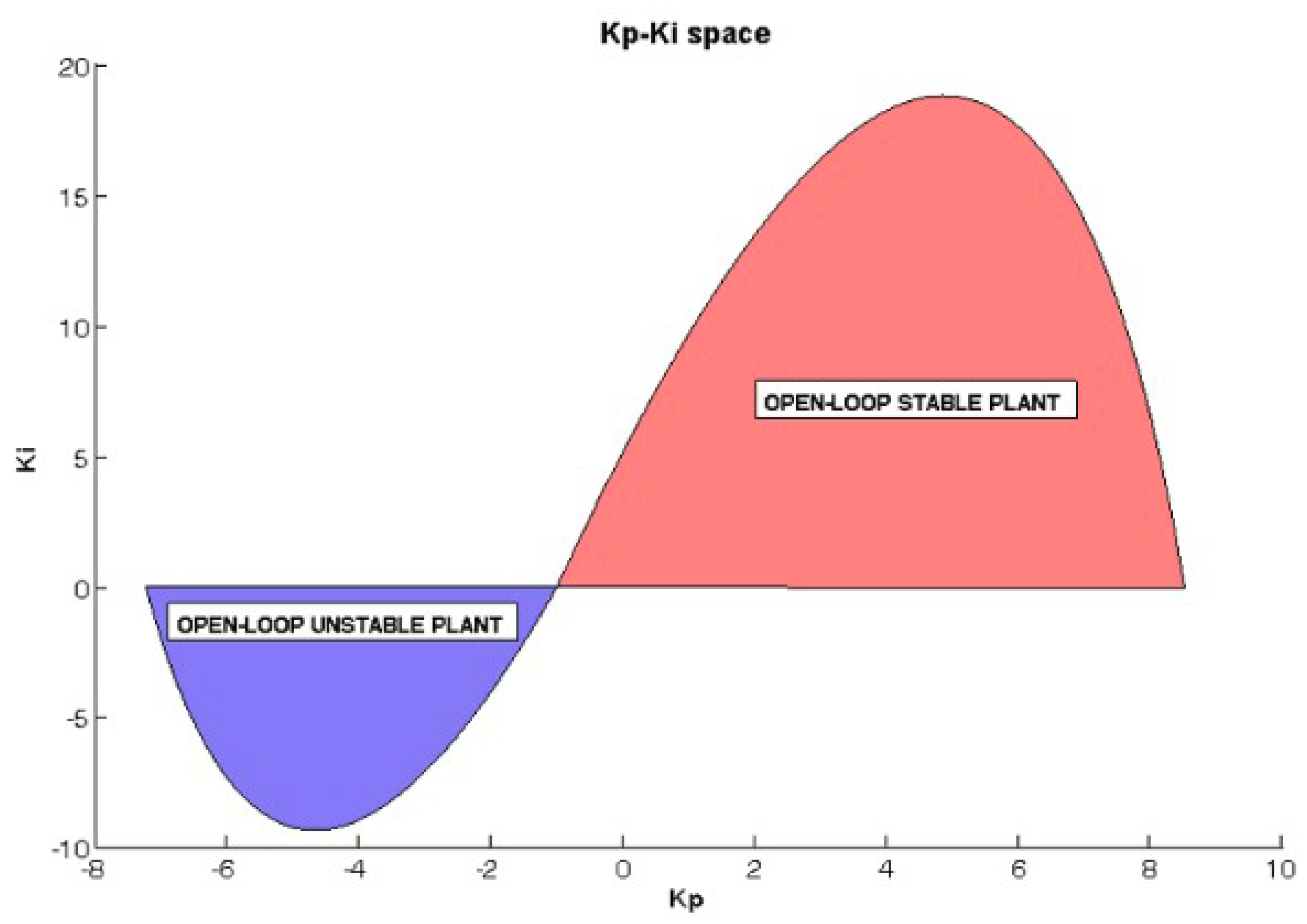
• K_P–K_I parameter space (b). This plot shows the K_P–K_I parameter space. The current K_P and K_I values are represented by a red point. These values are also shown in two text fields located on section f (see Figure 5). PI parameters can be modified either by editing these text fields or by dragging the aforesaid red point. In addition, the plot shows the set of PI controllers that stabilize the specified feedback system. If any of the model parameters are modified, the K_P–K_I region is automatically updated.
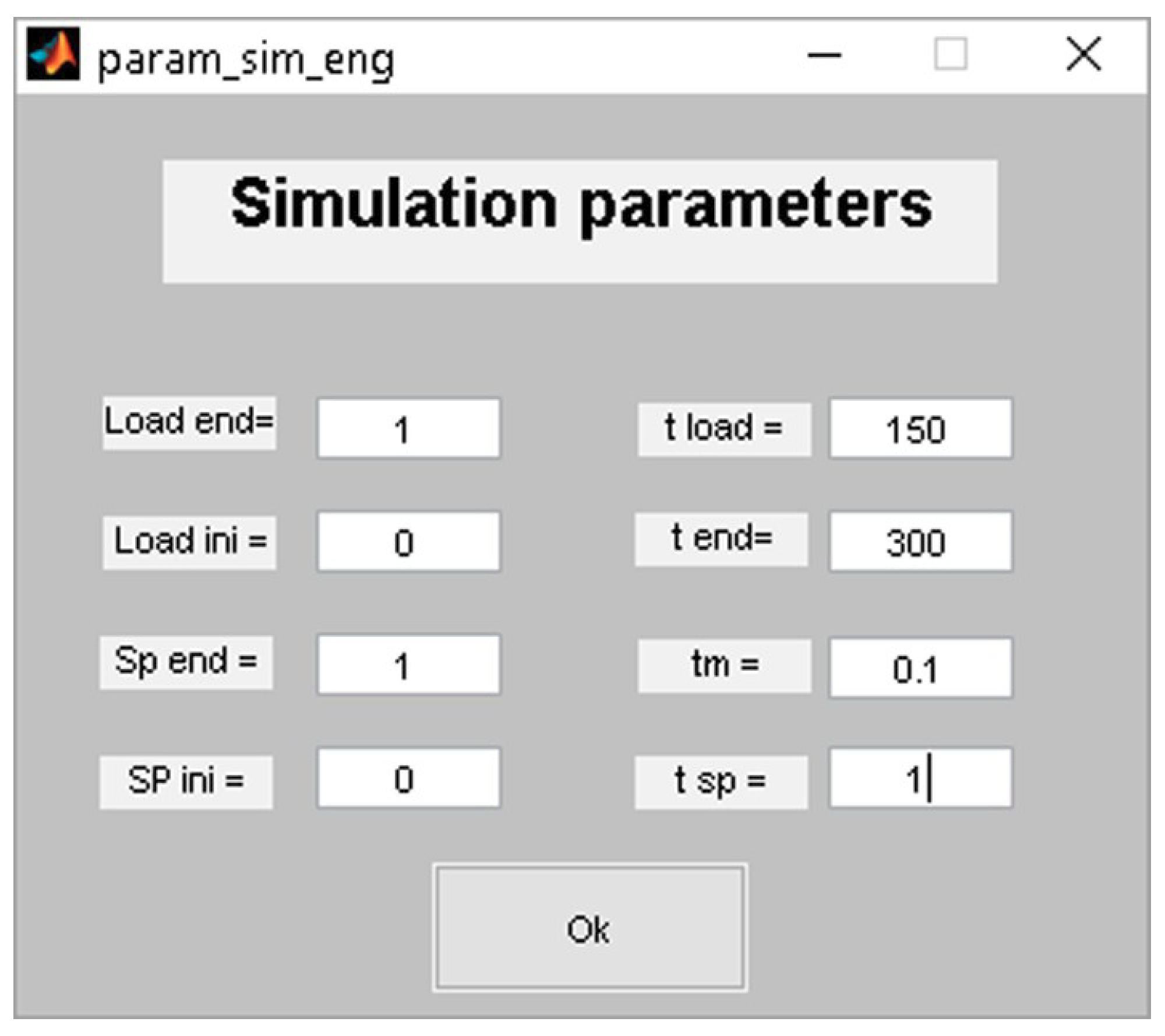
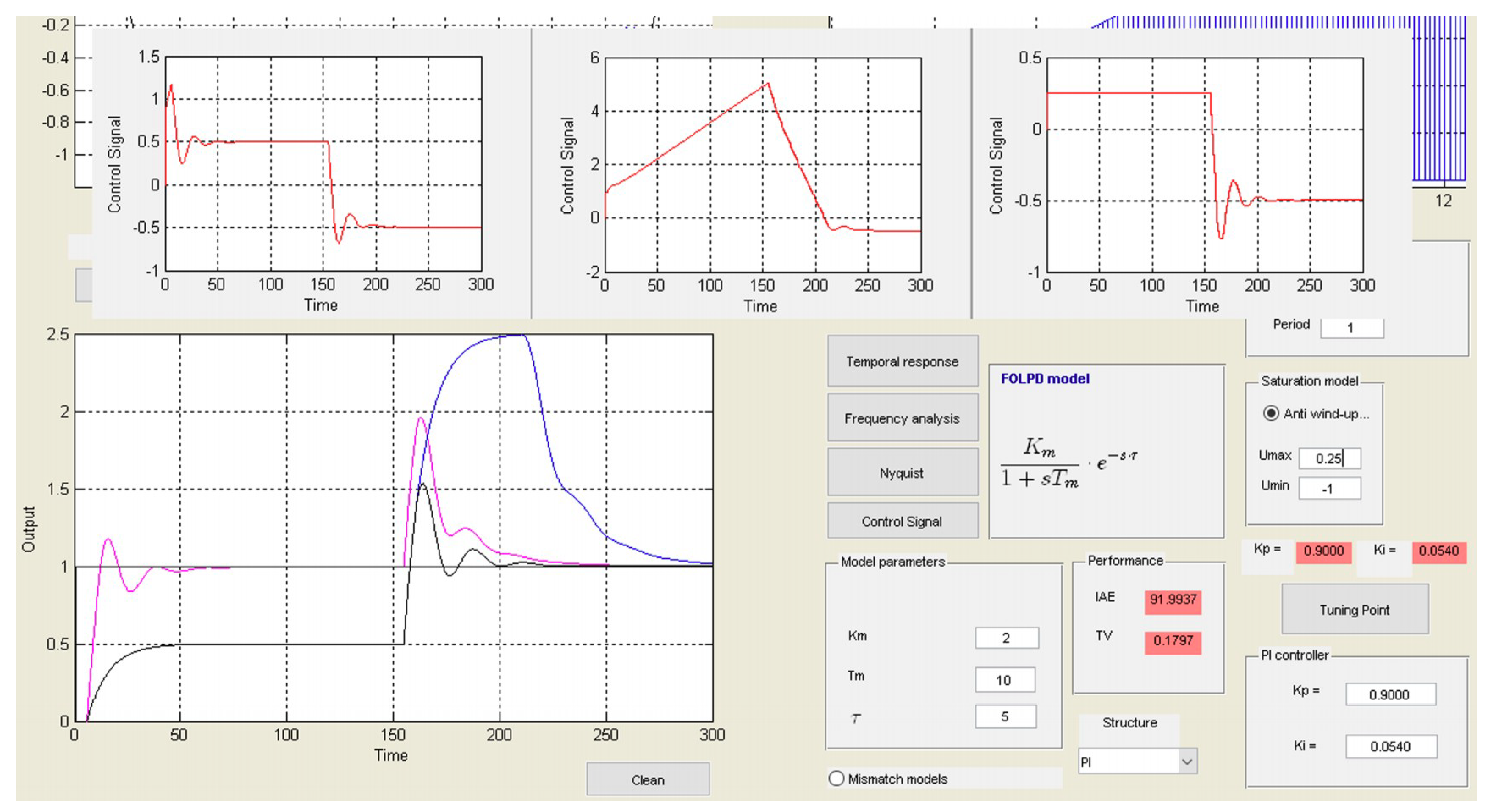
• Time response simulation (c). This plot shows the temporal response of the specified feedback system. It is possible to show different temporal responses, which is useful to contrast different tuning rules. The simulation parameters window (Figure 6) allows the user to configure step changes in both the reference signal and load disturbance. The initial and final values of these step changes, as well as the times when they occur, must be specified.
• Model parameters (d). As mentioned before, the model parameters (steady-state gain, time constant, and time delay) can be changed by editing the text fields contained in this panel. In addition, the tool can work with one or two models by clicking the radio-button Mismatch models. By default, only the “nominal” model is used. However, when the second one, the “simulation” model, is enable, the two models are used and provide the corresponding stability regions, the requested tuning rules are applied on the “nominal” model, and simulations and analysis are performed using the “simulation” model. Therefore, enabling the Mismatch models button, the user can modify these model parameters and analyze the robustness of the closed-loop system. This feature can be also used to consider process model uncertainties due to non-linearities of the plant. Although there are control methodologies directly accounting for the non-linear nature of the system [39,40], a classical approach is linearizing the original system around the nominal operation point, and assuming the non-linearities as parameter uncertainties of the approximated linear model when the point of operation changes.
• Tuning rules (e). The Tuning Rules menu, located on the upper part of the main window, contains the tuning rules described in

  Table A1. PI tuning rules for stable first order plus time delay (FOPTD) systems.

  Author Rule	KP	TI	Comment
  Ziegler and Nichols (1942)	$\frac{0.9T}{K\tau }$	$\frac{\tau }{0.3}$	Quarter decay ratio, $0.1\le \frac{\tau }{T}\le 1$
  AMIGO Aström and Hägglund (2005)	$\frac{0.15}{K}+\left(0.35-\frac{\tau T}{{\left(\tau +T\right)}^2}\right)\frac{T}{K\tau }$	$0.35\tau +\frac{13\tau T^2}{T^2+12\tau T+7{\tau }^2}$	I-P structure when $\frac{\tau }{\tau +T}\le 0.5$ otherwise PI structure
  MISE Murrill (1967)	$\frac{1.305}{K}{\left(\frac{T}{\tau }\right)}^{0.959}$	$\frac{T}{0.492}{\left(\frac{\tau }{T}\right)}^{0.739}$	Regulator tuning by minimum integral error $0.1\le \frac{\tau }{T}\le 1$
  MIAE Murrill (1967)	$\frac{0.984}{K}{\left(\frac{T}{\tau }\right)}^{0.986}$	$\frac{T}{0.608}{\left(\frac{\tau }{T}\right)}^{0.707}$
  MITAE Murrill (1967)	$\frac{1.305}{K}{\left(\frac{T}{\tau }\right)}^{0.959}$	$\frac{T}{0.492}{\left(\frac{\tau }{T}\right)}^{0.739}$
  MIAE Rovira et al. (1969)	$\frac{0.758}{K}{\left(\frac{T}{\tau }\right)}^{0.861}$	$\frac{T}{1.020-0.323\frac{\tau }{T}}$	Servo tuning by minimum integral error $0.1\le \frac{\tau }{T}\le 1$
  MITAE Rovira et al. (1969)	$\frac{0.586}{K}{\left(\frac{T}{\tau }\right)}^{0.916}$	$\frac{T}{1.030-0.165\frac{\tau }{T}}$
  Cohen and Coon (1953)	$\frac{1}{K}\left(0.9\frac{T}{\tau }+0.083\right)$	$T\left(\frac{3.33\frac{\tau }{T}+0.31{\left(\frac{\tau }{T}\right)}^2}{1+2.22\frac{\tau }{T}}\right)$	Quarter decay ratio, $0<\frac{\tau }{T}\le 1$
  O’Dwyer (2001)	$\frac{\pi T}{2A_{m}K\tau }$	$T$	Am: Gain margin
  Skogestad (2003)	$\frac{T}{K\left(T_c+\tau \right)}$	$\min \left(T,4\left(T_c+\tau \right)\right)$	Tc: Closed-loop time constant $T_c\le \left(T+\tau \right)$
  IMC Rivera et al. (1986)	$\frac{\left(T+\frac{\tau }{2}\right)}{K{T}_c}$	$T+\frac{\tau }{2}$	Tc: Closed-loop time constant $1.7\tau \le T_c\le \left(T+\tau \right)$

  and

  Table A2. PI tuning rules for unstable FOPTD systems.

  Author Rule	KP	TI	Comment
  Mahji and Atherton (2000)	$\frac{1}{K}\left(0.889+\frac{e^{\raisebox{1ex}{$-\tau $}\!\left/ \!\raisebox{-1ex}{$T$}\right.}-0.064}{e^{\raisebox{1ex}{$\tau $}\!\left/ \!\raisebox{-1ex}{$T$}\right.}-0.990}\right)$	$\frac{2.6316T\left(e^{\raisebox{1ex}{$\tau $}\!\left/ \!\raisebox{-1ex}{$T$}\right.}-0.966\right)}{e^{\raisebox{1ex}{$-\tau $}\!\left/ \!\raisebox{-1ex}{$T$}\right.}-0.377}$	ISTE optimization criterion $0<\frac{\tau }{T}<0.693$
  De Paor and O’Malley (1989)	$\frac{1}{K}\left(\cos \sqrt{\left(1-\frac{\tau }{T}\right)\frac{\tau }{T}}+\sqrt{\frac{T}{\tau }\left(1-\frac{\tau }{T}\right)}\sin \sqrt{\left(1-\frac{\tau }{T}\right)\frac{\tau }{T}}\right)$	$\frac{T}{\left[\sqrt{\frac{T}{\tau }\left(1-\frac{\tau }{T}\right)}\right]\tan \left(0.5\phi \right)}$$\phi ={\tan }^{-1}\sqrt{\frac{T}{\tau }\left(1-\frac{\tau }{T}\right)}-\sqrt{\left(1-\frac{\tau }{T}\right)\frac{\tau }{T}}$	Gain margin Am = 2 $\frac{\tau }{T}<1$
  Venkatashankar and Chidambaram (1994)	$\frac{1}{K}\sqrt{0.98\sqrt{1+\frac{0.04T^2}{{\left(T-\tau \right)}^2}}\left(\frac{25}{\tau }\right)\beta \left(T-\tau \right)\sqrt{\frac{1+\frac{{\beta }^2{T}^2}{{\tau }^2}}{1+{\beta }^2\frac{625}{{\tau }^2}{\left(T-\tau \right)}^2}}}$	$25\left(T-\tau \right)$	$\beta =1.373\mathrm{when}\frac{\tau }{T}<0.25$$\begin{array}{c}\beta =0.953\\ \mathrm{when}0.25\le \frac{\tau }{T}<0.67\end{array}$
  Chidambaram (1995)	$\frac{1}{K}\left(1+0.26\frac{\tau }{T}\right)$	$25T-27\tau$	$\frac{\tau }{T}<0.6$
  Chidambaram (1997)	$\frac{1.678}{K}\ln \left(\frac{T}{\tau }\right)$	$0.4015T{e}^{5.8\raisebox{1ex}{$\tau $}\!\left/ \!\raisebox{-1ex}{$T$}\right.}$
  Ho and Xu (1998)	$\frac{{\omega }_{p}T}{A_{m}K}$ ${\omega }_p=\frac{A_m{\Phi }_m+0.5\pi A_m\left(A_m-1\right)}{\left(A_m^2-1\right)\tau }$	$\frac{1}{1.57{\omega }_p-{\omega }_p^2\tau -\frac{1}{T}}$	Φm: Phase margin Am: Gain margin $\frac{\tau }{T}<0.62$

  . These tuning rules are organized in two sub-menus: open-loop stable models and open-loop unstable models. When a tuning rule is selected (and its validity range is fulfilled by the nominal model parameters), the tool automatically generates a point or a set of points in the K_P–K_I parameter space. Depending on the tuning rule, some extra information can be requested by means of a pop-up menu, such as gain margin, phase margin, or the closed-loop time constant. The generated points are tagged in the K_P–K_I parameter space with the name of the tuning rule and the design specification. All these points are also updated when model parameters are modified.
• PI controller configuration (f). A set of control panels related with the PI controller are included in this section. The Control Design panel allows selecting between the continuous and discrete domains. As mentioned before, in this tool, the PI design is performed in the continuous domain. Thus, once the design is carried out (i.e., the PI parameters and the model parameters are defined), the performance and degradation of the time response can be analyzed by clicking on the discrete radio-button. A new simulation will then be executed according to the sampling period defined in the Period text field. In addition, when the user switches from the continuous to the discrete domain, the plot that displayed the K_P–K_I parameter space region will display the closed-loop discrete pole localizations within the Z-plane. The saturation model can be specified in the Saturation model panel, where an anti-windup strategy can be enabled, and the minimum and maximum process input values can be specified. The saturation model is only applied when the discrete domain is selected. The tool can work with two types of PI structures: PI and I-P. In the I-P structure, only the measured output is introduced in the proportional term, and not the error, as in the PI structure. The K_P and K_I values are always visible in the text fields of the PI controller panel. As mentioned in point 2), they are also represented by the red point in the K_P–K_I parameter space. The Tuning point push button updates the control parameters with the K_P and K_I values shown in the text fields of pink color. These text fields show the obtained values by the last tuning rule selected by the user. In all cases, the temporal and frequency responses are updated. Finally, each time a simulation is carried out, the text fields contained in the Performance panel are updated. These field texts contain the integral of absolute error (IAE) and the total variation (TV). The first measure is useful to evaluate the output control performance, and the second to evaluate the “smoothness” of the control signal.
• Secondary windows (g). The control signal, the Nyquist plot, and the frequency response features (gain margin, phase margin, and sensitivity and complementary sensitivity peaks) are only displayed when the user demands them by means of the respective push buttons placed on the center of the main window. After changing the model or controller parameters, these windows are quickly updated. These windows are shown in Figure 7.

The tool provides an additional feature to analyze the tuning rules. Below the model parameter space, the edit text field named line τ/T_m allows plotting lines with different slopes τ/T. This feature is useful to test the validity range of different tuning rules. Similarly, using the edit text field named line τ/T_I, lines with different slopes K_I/K_P can be plotted in the K_P–K_I parameter space, and pole cancellation methodologies can be applied. In addition, the user can zoom or pan the different axes, save and load sessions, or export the controller or the process model to the MATLAB workspace.

3.1. Comparison with Similar Software and Main Novelties of the Proposed Tool

The tool has been designed following the guidelines of similar tools, such as PIDLab [41], the PID Tuner application from MATLAB, or the PID interactive learning modules based on Sysquake [24,28]. The main common features are the following:

• Modification of the process model and the controller parameters.
• Simulation parameters configuration.
• Representation of the closed-loop temporal response (control signal and controlled variable).
• Representation of the system frequency response (Nyquist diagram).
• Performance indices computation (IAE, TV).
• Interactive zooming/panning.

The main contributions of the proposed tool, that distinguishes it from others, can be summarized in the following features:

• The tool gathers several rules of tuning of PI controllers for FOPTD systems to allow their comparative analysis. Although some applications, such as MATLAB PID Tuner tool, allows adjustment with tuning rules, it only has 4 implemented. The present tool contains 17 rules with the future possibility to increase that number or add custom-user tuning rules.
• K_P–K_I controller parameter space and stability region. This special feature allows the user to choose the controller parameters interactively. Along with it we can also show the curves of different specifications, facilitating the previous task. Furthermore, several tuning rules can be compared by means of their associated points, which can be displayed in the mentioned region.
• Stability region in the parameter space of the T–τ model. For a gain process K and a given PI controller, this region shows the set of T–τ combinations that the controller is able to stabilize. Thus, the two aforementioned stability regions are very useful to study the robustness of the system.
• In addition to the continuous time domain analysis, the tool allows checking the performance of the closed-loop system in the discrete domain, taking into consideration real aspects in the controller implementation, such as the selection of sampling period, definition of the control signal limits, or the activation of an anti-windup method.

3.2. Training or Educational Uses

There are different uses supported by the tool, such as the following ones:

• Trial-and-error tuning, by means of the stabilizing region. The stabilizing region in the K_P–K_I parameter space is provided by the tool. By moving the red point within this space, the system stability and closed-loop response can be studied as a function of the control parameters.
• Comparison of PI tuning rules. The user can easily compare the performance achieved with different tuning rules and different specifications.
• Testing PI control limitations. For instance, in the case of an unstable FOPTD model, the user can check that it is not possible to achieve large gain and phase margins by moving the red point inside the corresponding stabilizing region (K_P–K_I parameter space). Similarly, the user can observe the set of FOPTD processes that can be stabilized given a particular PI controller.
• Analysis of PI controllers designed by pole cancellation. There are tuning rules that cancel the model pole with the controller zero doing T_I = T. By specifying a line 1/T_I in the K_P–K_I parameter space and moving the red point along it, PI controllers designed by pole cancellation can be studied; where T_I remains constant, and only K_P is changing.
• Robust analysis of the closed-loop system. As mentioned before, the tool can work simultaneously with the nominal and simulation models. Thus, when the Mismatch models radio-button is enabled, the user can analyze perturbations in the model parameter space and study the stabilizing regions or the frequency and temporal responses of the closed-loop system.
• Effects of practical considerations. As mentioned before, real considerations of PI controllers have been taken into account. In addition of the effects of a poor choice of the controller parameters, the degradation of the system closed-loop response when the sample time is not properly selected can be studied.

4. Illustrative Example

This section describes an example using the tool. The goal is controlling a stable FOPTD system by means of a PI controller. The process is given by the transfer function in (10). Different PI tuning rules are compared and, once a design is selected, its discrete implementation is tested analyzing possible practical problems.

$$G\left(s\right)=\frac{2·e^{-5s}}{10s+1}$$

(10)

First, the process information is introduced in the Model Parameters panel of the main window setting 2, 10, and 5 in the respective textboxes K_m, T_m, and τ. Immediately, the stabilizing region in the K_P–K_I space for this system is calculated. The corresponding one for this example is shown in Figure 5. For the simulations, the parameters provided in Figure 6 are configured. There are step changes from zero to one in the set-point, and the load disturbance at times t = 1 s and t = 150 s, respectively. The simulation time is 300 s.

In this example, three tuning rules for a stable open-loop process are selected: AMIGO, Ziegler–Nichols, and O’Dwyer (with a gain margin of 3 as specification). The corresponding PI parameters are collected in

Table 2. PI parameters and performance indices.

Tuning Rule	KP	KI	IAE	TV	GM	PM
AMIGO	0.021	0.022	67.87	1.32	7.6	75.7
O’Dwyer	0.524	0.052	29.78	1.74	3	60
Ziegler–Nichols	0.9	0.054	29.67	3.47	1.9	54.4

. These can be also identified in the K_P–K_I space in Figure 5. Their closed-loop responses are shown in section c) of Figure 5 (AMIGO in pink, O’Dwyer in blue, and Ziegler–Nichols in black), and several performance indices are gathered in Table 2. Using the AMIGO tuning rule, the response is the slowest of the three, and it has the higher IAE value. However, it does not show overshoot, and has better robustness with the higher gain and phase margins. The responses using the Ziegler–Nichols rule or O’Dwyer rule are faster, and have smaller IAE values. Nevertheless, they show an overshoot and lower gain and phase margins. Note that the design using O’Dwyer rule achieves the specified GM of 3.

Assuming that the design obtained by the Ziegler–Nichols rule is the preferred one, the next stage is translating it into a discrete implementation. After selecting the Discrete option in the Control Design panel, the figure of the K_P–K_I space is substituted by the stability area with the closed-loop poles in the discrete space. To determine a proper sampling time, the Nyquist-Shannon criterion states that the sampling rate must be twice the largest frequency contained in the signal spectral content. In control, a typical rule of thumb is to apply a sampling frequency of 5 to 10 times the bandwidth of the closed-loop system, to avoid degradation of the response. In this example, assuming the original design in the continuous domain, the closed-loop bandwidth is about 0.4 rad/s. Considering 10 times this value, a proper sample time h must be less than 2·π/4 = 1.57 s. In this example, two sample times are selected: one of 1 s, fulfilling the previous condition; and the other of 10 s, not satisfying the criterion. As shown in Figure 8, for a sample time of 1 s, the closed-loop poles lay inside the unit circle, which is necessary for stability. The corresponding closed-loop response is also shown in the bottom left corner (in black), together with the response obtained with a sample time of 10 s (in blue). In the first case, a sample time of 1 s is acceptable; however, the response is considerably deteriorated with a sample time of 10 s. It can be checked that the closed-loop response becomes unstable for sample times greater than 18 s (with closed-loop poles outside the unit circle).

Finally, Figure 9 shows the simulation results when the process input has a maximum limit u_max of +0.25, and a minimum one u_min of −1. The pink line represents the ideal closed-loop response without any constraints. The blue one is the response with the previous limitations, and the black one is the response with the control signal constraints and an anti-windup method in the PI controller. The corresponding control signals are also shown in the top of the figure, from left to right, respectively.

When there are no constraints, the reference is achieved quickly; however, it can be appreciated that the control signal is out of range. It only returns to range after the step change in the load disturbance takes place in order to reject it. With process input limitations and no anti-windup, the reference initially is not reached because the control signal is saturated. However, since the error remains constant, the integral control part keeps increasing. This fact produces windup in this signal and, after the load step at t = 150 s, the real process input does not change until 100 s later, when the internal control signal decays to below 0.25. Consequently, the time to reject the disturbance and reaching the set-point is very large. This response is considerably improved by means of the anti-windup algorithm of Table 1. In this case, the reference is not reached at the beginning; however, the control signal is internally limited to its upper bound, and then reacts very quickly after the load disturbance step. Thus, the set-point is achieved sooner, and the windup problem is avoided.

4.1. Practical Laboratory Process

As part of a practical case study, students were asked to apply a set of tuning rules in one of our laboratory processes by using the developed tool. The results obtained by simulation were compared to those obtained in the process. As shown in Figure 10, the experimental plant consists of a control flow rate in a closed circuit, where water is pumped and returned to a tank. The main components are a water tank, a three-phase pump which takes the water from the bottom of the tank and returns it, an electromagnetic flow sensor which measures the flow rate to be controlled, and a set of tubes and valves for the circuit connection. At the outlet of the pump there are two branches, so that one part of the water flow taken is returned to the tank by a first branch and the other part goes through the other branch where the flow meter is located. In this way, the maximum flow rate that circulates by the second branch can be adjusted. The system incorporates a variable frequency drive (VFD) to regulate the water flow rate. Finally, a programmable automation controller (PAC) is used for the implementation of the control strategy. The flow sensor output and the VFD input are connected to the PAC. The plant is also connected to a PC where the process is monitored, and the PI control parameters are specified. The process variable to control is the flow rate, and the manipulated variable is the frequency at which the pump operates. The sampling period of all the process variables is 0.5 s.

First, the following FOPTD model was identified for an operational point of 20 Hz (with a fitness of 90%):

$$G\left(s\right)=\frac{2.0875·e^{-1.95s}}{2.33s+1}.$$

(11)

This process model was used with the developed tool. The AMIGO, Ziegler–Nichols, and Murrill (minimal IAE-servo) tuning rules were applied, obtaining the corresponding K_P and K_I parameters. The experimental and simulated step responses for each tuning rule are shown in Figure 11.

As can be seen from Figure 11, there is a great similarity between the experimental (a) and simulated (b) step responses. The design using the AMIGO rule provides the slowest response without oscillations. The responses using the MIAE (Murrill minimal ITAE-servo) and Ziegler–Nichols tuning rules show a similar rising time. The MITAE tuning rule shows a small overshoot in simulation which is not present in the corresponding real response. Finally,

Table 3. Control parameters and performance obtained from the lab test.

Tuning Rule	KP	KI	IAE	TV	IAEREAL	TVREAL
Murril (min. ITAE-servo)	0.3304	0.1265	19.77	2.05	20.90	1.92
AMIGO	0.1302	0.0573	41.78	1.80	46.30	1.78
Ziegler–Nichols	0.5152	0.0793	29.97	3.65	29.81	3.62

shows the K_P and K_I parameters obtained with the tool. The last two columns show the IAE and TV performance indices computed with the tool and from real data, respectively. As can be noted, there is a good correspondence between the real and simulated indices.

5. Assessment and Evaluation

Electronic engineering students at the University of Cordoba conducted a set of exercises using the developed tool. For the evaluation of the tool, the students were asked to complete an electronic questionnaire. The details of the survey carried out are explained in this section.

5.1. Student Survey

As mentioned in [42], interactive tools should be easy to understand and use, provide a good visual sensation, consider real-life problems, and highlight the essential theoretical ideas by means of a pedagogical guideline. These requirements have been addressed as follows:

• Theoretical ideas: The tool is mainly focused on the design of PI controllers for stable and unstable FOPTD systems and the application of different tuning rules. However, it has been developed to facilitate the learning other basic concepts related to process control, such as stability boundary, robustness, temporal response for reference tracking, disturbance rejection, frequency response (Nyquist plot), and different closed-loop performance indices.
• User-friendly interface: The graphical user interface (GUI) has been designed avoiding unnecessary elements. In addition, an introduction to the tool is given to the students based on the workflow shown in Figure 4.
• Real-life problem: The discrete implementation of PI controllers can be evaluated in the tool considering real aspects, such as the windup effect of process input constraints. This step can be carried out after a proper tuning is performed (see Figure 4), allowing one to study the possible performance degradations in the closed-loop system response.
• Visual sensation: The GUI is structured coherently and is user-friendly, trying to keep the interface simple, and ensuring that the possible actions that can be carried out are easy to understand.

The proposed tool has been used in the corresponding lesson about PID/PI controllers of the Automatic Control subject. This lesson is composed of face-to-face instructions (4 h), a practical lab exercise and virtual homework. The theoretical parts of the instructions comprise of four lessons of 1 h: (a) Introduction on PID controllers, different control actions, tuning parameters, different architectures (ideal, series, parallel), and so on; (b) PID/PI controller design using tuning rules; (c) PID controller tuning based on the root loci; and (d) PID tuning methodologies on the frequency domain. The tool is mainly used in point (b), whose contents are explained in a computer lab following these points:

• Introduction of PID/PI tuning rules, their classification, explanation of the most extended rules, and advantages and disadvantages.
• Description of the tool based on the workflow shown in Figure 4.
• Running the tool which is available to students, and resolution and discussion of several examples interactively.
• Brief introduction to the discrete implementation of controllers and practical aspects, such as sample time selection and input saturations and wind up effect. The fundamentals of these concepts are explained in detail in advanced control subjects. In this lesson, these problems are exemplified using the tool.

The students also have to carry out, in pairs, a lab exercise similar to the one described in Section 4.1. They must work autonomously at the Automatic Control laboratory in the last weeks of the course. The proposed exercise involves:

• Description of the process to be controlled and its operation.
• Obtaining a model of the system by identification and approximation to a FOPTD model.
• Design and simulation of different PI controllers using the proposed tool.
• Verification of the previous designs in the real process and comparison with simulation results.

Finally, extra exercises are proposed as homework using the online learning platform. Some of them are prepared to be performed using the proposed tool, as it is explained later. Three subscales were differentiated in the electronic questionnaire requested to the students: Learning value, Value added, and Design usability and easy understanding of the tool. These items are explained as follows:

• Learning value considers questions about the students’ perceptions of the effectiveness of the proposed tool in facilitating the learning of PI control theory.
• Value added evaluates the use of the tool as a complement for traditional lectures.
• Design usability and easy understanding of the tool is aimed to evaluate how the students perceive the clarity and ease to work with the GUI.

The main objective of the questions carried out was to analyze the contribution of the proposed tool on improving the learning process about control theory and specifically PI controllers. Assessment and evaluation were based on [27,43,44,45]. The questionnaire carried out is shown in

Table 4. Student questionnaire for tool assessment.

Learning Value
Q1	Did the tool facilitate you to understand new concepts of PI control and FOPTD processes?
Q2	Evaluate if the tool helps you to remember basic concepts about PI control theory.
Q3	Evaluate if you consider the tool useful as a complement of lecture explanations and if it motivates you to learn the explained control concepts.
Value added
Q4	Did you like the practical simulations carried out with the tool?
Q5	Rate if you think you have improved your theoretical knowledge about tuning rules for PI controllers.
Q6	Did the tool help you to understand the practical issues that can arise when implementing a PI control loop?
Q7	Rate the interactive capabilities of the tool.
Design usability and easy understanding of the tool
Q8	Is the graphical user interface of the tool user-friendly?
Q9	Rate if the tool is easy to understand and use.
Q10	Do you think the concepts explained with the tool were easy to follow?

.

The students’ answers are shown in

Table 5. Students’ responses of the tool survey (number of students = 34).

Group Items	Strongly Disagree	Disagree	Neutral	Agree	Strongly Agree
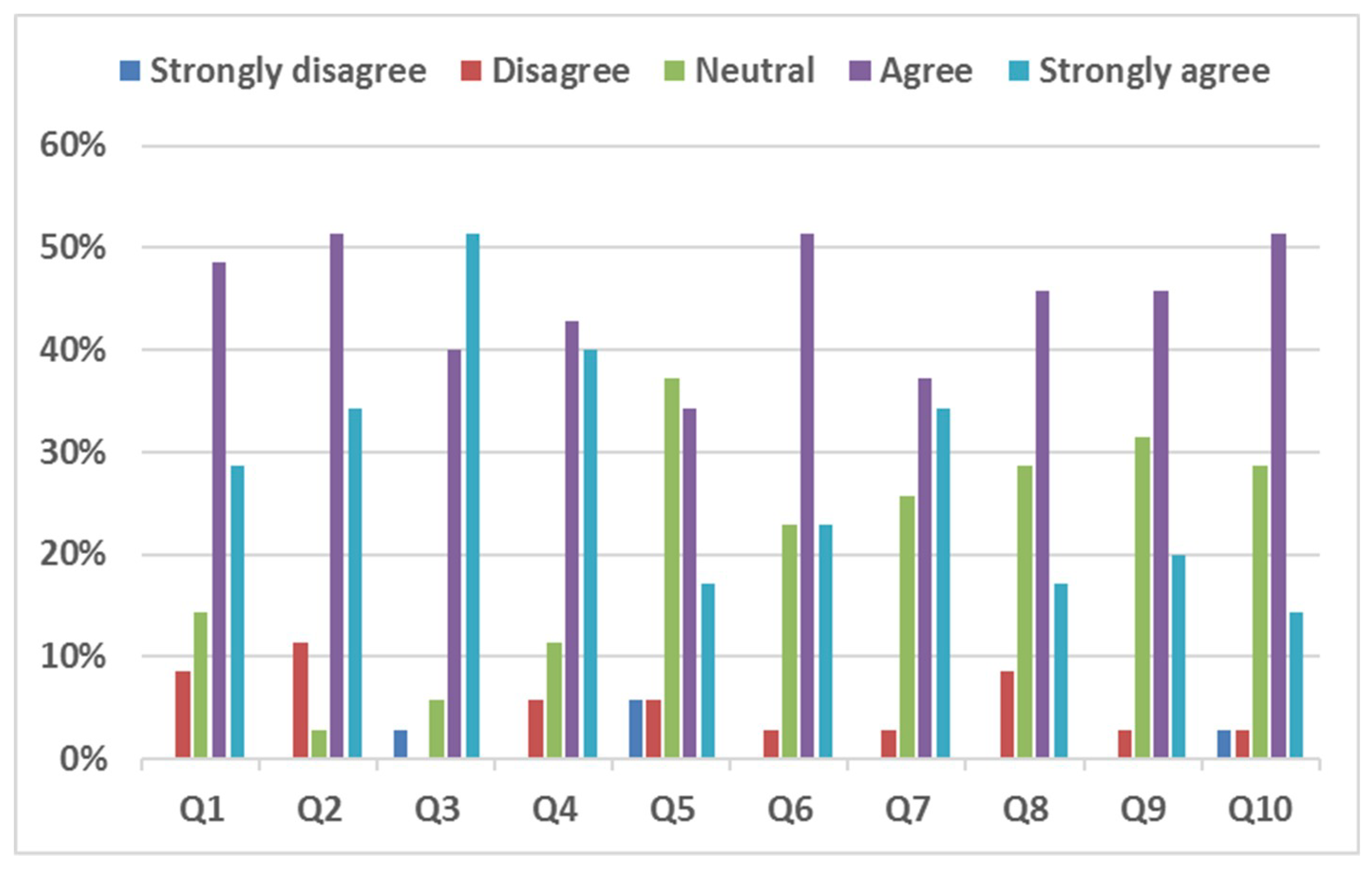
Learning value (Q1, Q2, Q3)	0%	7%	8%	47%	38%
Value added (Q4, Q5, Q6, Q7)	1%	4%	24%	41%	29%
Design usability and easy understanding of the tool (Q8, Q9, Q10)	0%	5%	30%	48%	17%

. A Likert scale was used, rated as strongly agree, agree, neutral, disagree, or strongly disagree. The students’ survey answers are shown in Figure 12. The relatively high rates of answers for the options “Strongly agree” and “Agree” are good indications supporting the use of the proposed tool for the learning and strengthening of new concepts about PI control theory. The percentages obtained in the Learning value group items suggest that most students think that basic concepts about PI controllers are clearly presented and explained. Although the “Agree” response shows the highest percentage in practically all the questions, it is also important to remark the high percentage of “Neutral” responses in the second and third groups. This fact is especially evident in questions Q5, Q8, and Q10, where the results are not so good as expected. Therefore, from the survey results, future tool enhancements can be considered. The authors think that the results in these three questions are mainly derived from the way in which the tool was introduced and presented to the students. Since this is the first course where the tool is used for undergraduate students, refining the tool integration into the subject contents in the next years will help to improve the students’ experience with the tool. In addition, the incorporation of more tuning rules can be taken into account as another future improvement.

5.2. Student Results

Thirty-four of the 43 students in class carried out the aforementioned exercises voluntarily. These exercises consisted of concept questions and basic problems about PI controller design, covering the material taught in class. Note that the students did not possess prior background on control theory. The proposed exercises are similar to the illustrative example described in Section 4. First, given a process model and simulation parameters, students are asked to configure the tool with these data. Then, they must perform the PI controller design using different tuning rules and compare the corresponding performance and robustness of the control system by means of the stability regions and indices provided by the tool. Next, after selecting a specific PI design, they must evaluate the controller performance using a discrete implementation. Practical aspects, such as sample time, input saturations, and anti-windup, are considered at this stage. These exercises ask the students to modify these parameters to check their impact on the control system performance and test the degradation of the closed-loop response when improper values are chosen. Finally, an exercise focused on an unstable process is included. Similar to the first exercise, different tuning rules are tested and compared; however, the main aim of this exercise is to show the students that these processes are more difficult to control, their corresponding stability regions are more constrained with limited minimum and maximum values for the controller gain and, consequently, they achieve larger performance specifications, such as overshoot and settling time. In all the exercises, different controller parameters and performance indices are requested to assess students’ progress. The answers to the exercises were submitted through the online learning platform Moodle, implemented at the University of Cordoba [46]. Figure 13 shows the mark distribution of the 34 students who submitted the proposed exercises. The average mark was 7.7, with a standard deviation of 1.9. This is good indicator on the students’ ability to resolve the proposed exercises by means of the developed tool.

6. Conclusions

In this paper, an interactive software tool specially focused on PI controllers was presented. It contains several PI tuning rules for stable and unstable FOPTD processes. The tool has been developed, taking into account practical considerations, and can be used both academically and in real cases. Assessment data and student feedback indicate that the learning objectives were achieved. The feedback from students was positive, which suggests that the presented tool is a good complement for traditional lectures of basic control concepts and practical problems related to PI controller implementation. Future work will be mainly dedicated to adding new functionalities to the tool, such as the capacity of including custom-user PI tuning rules.

References

- Srivastava, S.; Pandit, V.S. A PI/PID controller for time delay systems with desired closed loop time response and guaranteed gain and phase margins. J. Process Control 2016, 37, 70–77. [Google Scholar] [CrossRef]
- Knospe, C. PID control. IEEE Control Syst. 2006, 26, 30–31. [Google Scholar] [CrossRef]
- Huba, M.; Vrančič, D. Comparing filtered PI, PID and PIDD 2 control for the FOTD plants. IFAC-PapersOnLine 2018, 51, 954–959. [Google Scholar] [CrossRef]
- Alcántara, S.; Vilanova, R.; Pedret, C. PID control in terms of robustness/performance and servo/regulator trade-offs: A unifying approach to balanced autotuning. J. Process Control 2013, 23, 527–542. [Google Scholar] [CrossRef]
- O’Dwyer, A. An Overview of Tuning Rules for the PI and PID Continuous-Time Control of Time-Delayed Single-Input, Single-Output (SISO) Processes. In PID Control in the Third Millenium; Springer: London, UK, 2012; pp. 3–44. [Google Scholar]
- O’Dwyer, A. Handbook of PI and PID Controller Tuning Rules, 2nd ed.; Imperial College Press: London, UK, 2006; ISBN 9781860949104. [Google Scholar]
- Leva, A.; Maggion, M. Model-Based PI(D) Autotuning. In PID Control in the Third Millenium; Springer: London, UK, 2012; pp. 45–73. [Google Scholar]
- Li, Y.; Ang, K.H.; Chong, G.C.Y. Patents, Software, and Hardware for PID Control: An Overview and Analysis of the Current Art. IEEE Control Syst. 2006, 26, 42–54. [Google Scholar] [CrossRef]
- Silva, G.J.; Datta, A.; Bhattacharyya, S.P. PID Controllers for Time-Delay Systems; Birkhäuser: Basel, Switzerland, 2005; ISBN 0817642668. [Google Scholar]
- Ziegler, J.G.; Nichols, N.B. Optimum settings for automatic controllers. Trans. ASME 1942, 64, 759–768. [Google Scholar] [CrossRef]
- Arrieta, O.; Vilanova, R. Simple PID tuning rules with guaranteed Ms robustness achievement. IFAC Proc. Vol. 2011, 44, 12042–12047. [Google Scholar] [CrossRef]
- Murill, P.W. Automatic Control of Processes; International Textbook, Co.: Scranton, PA, USA, 1967. [Google Scholar]
- Rovira, A.A.; Murrill, P.W.; Smith, C.L. Tuning controllers for setpoint changes. Instrum. Control Syst. 1969, 42, 67–69. [Google Scholar]
- Awouda, A.E.A.; Bin Mamat, R. Refine PID tuning rule using ITAE criteria. In Proceedings of the 2nd International Conference on Computer and Automation Engineering (ICCAE), Singapore, 26–28 February 2010; Volume 5, pp. 171–176. [Google Scholar]
- Hägglund, T.; Åström, K.J. Revisiting the Ziegler-Nichols tuning rules for PI control. Asian J. Control 2002, 2, 364–380. [Google Scholar] [CrossRef]
- Åström, K.J.; Hägglund, T. Revisiting the Ziegler–Nichols step response method for PID control. J. Process Control 2004, 14, 635–650. [Google Scholar] [CrossRef]
- Ho, M.-T.; Datta, A.; Bhattacharyya, S.P. Robust and non-fragile PID controller design. Int. J. Robust Nonlinear Control 2001, 11, 681–708. [Google Scholar] [CrossRef]
- Alfaro, V.M.; Vilanova, R. Optimal robust tuning for 1DoF PI/PID control unifying FOPDT/SOPDT models. In Proceedings of the 2nd IFAC Conference on Advance in PID control (PID’12), Brescia, Italy, 28–30 March 2012; Volume 2, pp. 572–577. [Google Scholar]
- Cho, W.; Lee, J.; Edgar, T.F. Simple analytic proportional-integral-derivative (PID) controller tuning rules for unstable processes. Ind. Eng. Chem. Res. 2013, 53, 5048–5054. [Google Scholar] [CrossRef]
- Rajinikanth, V.; Latha, K. Tuning and retuning of PID controller for unstable systems using evolutionary algorithm. ISRN Chem. Eng. 2012. [Google Scholar] [CrossRef]
- Rajinikanth, V.; Latha, K. Setpoint weighted PID controller tuning for unstable system using heuristic algorithm. Arch. Control Sci. 2012, 22, 481–505. [Google Scholar] [CrossRef]
- Korsane, D.T.; Yadav, V.; Raut, K.H. PID tuning rules for first order plus time delay system. Int. J. Innov. Res. Electr. Instrum. Control Eng. 2014, 2, 582–586. [Google Scholar]
- Vilanova, R.; Alfaro, V.M.; Arrieta, O. Robustness in PID Control. In PID Control in the Third Millenium; Springer: London, UK, 2012; pp. 113–146. [Google Scholar]
- Guzman, J.L.; Costa-Castello, R.; Dormido, S.; Berenguel, M. An Interactivity-Based Methodology to Support Control Education: How to Teach and Learn Using Simple Interactive Tools [Lecture Notes]. IEEE Control Syst. 2016, 36, 63–76. [Google Scholar] [CrossRef]
- Martínez, J.; Padilla, A.; Rodríguez, E.; Jiménez, A.; Orozco, H. Diseño de Herramientas Didácticas Enfocadas al Aprendizaje de Sistemas de Control Utilizando Instrumentación Virtual. Rev. Iberoam. Automática e Informática Ind. RIAI 2017, 14, 424–433. [Google Scholar] [CrossRef]
- Ruiz, Á.; Jiménez, J.E.; Sánchez, J.; Dormido, S. Design of event-based PI-P controllers using interactive tools. Control Eng. Pract. 2014, 32, 183–202. [Google Scholar] [CrossRef]
- Morales, D.C.; Jiménez-Hornero, J.E.; Vázquez, F.; Morilla, F. Educational tool for optimal controller tuning using evolutionary strategies. IEEE Trans. Educ. 2012, 55, 48–57. [Google Scholar] [CrossRef]
- Guzmán, J.L.; Aström, K.J.; Dormido, S.; Hägglund, T.; Berenguel, M.; Piguet, Y. Interactive learning modules for PID control. IEEE Control Syst. Mag. 2008, 28, 118–134. [Google Scholar] [CrossRef]
- Guzmán, J.L.; Dormido, S.; Berenguel, M. Interactivity in education: An experience in the automatic control field. Comput. Appl. Eng. Educ. 2013, 21, 360–371. [Google Scholar] [CrossRef]
- Aliane, N. A matlab/simulink-based interactive module for servo systems learning. IEEE Trans. Educ. 2010, 53, 265–271. [Google Scholar] [CrossRef]
- Mathworks Home Page. Available online: http://www.mathworks.com (accessed on 2 August 2016).
- Ruz, M.L.; Morilla, F.; Vázquez, F. Teaching control with first order time delay model and PI controllers. In Proceedings of the 8th IFAC Symposium on Advances in Control Education, Kumamoto, Japan, 21–23 October 2009; Volume 8, pp. 31–36. [Google Scholar]
- Garrido, J.; Ruz, M.L.; Morilla, F.; Vázquez, F. Interactive Tool for Frequency Domain Tuning of PID Controllers. Processes 2018, 6, 197. [Google Scholar] [CrossRef]
- Skogestad, S. Simple analytic rules for model reduction and PID controller tuning. J. Process Control 2003, 13, 291–309. [Google Scholar] [CrossRef]
- Åström, K.J.; Hägglund, T. Advanced PID Control; ISA-The Instrumentation, Systems, and Automation Society: Research Triangle Park, NC, USA, 2005. [Google Scholar]
- Ho, W.K.; Xu, W. PID tuning for unstable processes based on gain and phase-margin specifications. IEE Proc. Control Theory Appl. 1998, 145, 392–396. [Google Scholar] [CrossRef]
- Padma Sree, R.; Srinivas, M.N.; Chidambaram, M. A simple method of tuning PID controllers for stable and unstable FOPTD systems. Comput. Chem. Eng. 2004, 28, 2201–2218. [Google Scholar] [CrossRef]
- Seshagiri Rao, A.; Chidambaram, M. PI/PID Controllers Design for Integrating and Unstable Systems. In PID Control in the Third Millenium; Springer: London, UK, 2012; pp. 45–74. [Google Scholar]
- Pappalardo, C.M.; Guida, D. Adjoint-Based Optimization Procedure for Active Vibration Control of Nonlinear Mechanical Systems. J. Dyn. Syst. Meas. Control 2017, 139, 081010. [Google Scholar] [CrossRef]
- Pappalardo, C.; Guida, D. System Identification Algorithm for Computing the Modal Parameters of Linear Mechanical Systems. Machines 2018, 6, 12. [Google Scholar] [CrossRef]
- Rex Controls s.r.o PIDlab. Available online: www.pidlab.com (accessed on 31 October 2018).
- Balchen, J.G.; Handlykken, M.; Tysso, A. The need for better laboratory experiments in control engineering education. IFAC Proc. Vol. 1981, 14, 3363–3368. [Google Scholar] [CrossRef]
- Dormido, R.; Vargas, H.; Duro, N.; Sánchez, J.; Dormido-Canto, S.; Farias, G.; Esquembre, F.; Dormido, S. Development of a web-based control laboratory for automation technicians: The three-tank system. IEEE Trans. Educ. 2008, 51, 35–44. [Google Scholar] [CrossRef]
- Sánchez, J.; Dormido, S.; Pastor, R.; Morilla, F. A Java/Matlab-Based Environment for Remote Control System Laboratories: Illustrated with an Inverted Pendulum. IEEE Trans. Educ. 2004, 47, 321–329. [Google Scholar] [CrossRef]
- Fragoso, S.; Ruz, M.L.; Garrido, J.; Vázquez, F.; Morilla, F. Educational software tool for decoupling control in wind turbines applied to a lab-scale system. Comput. Appl. Eng. Educ. 2016, 24, 400–411. [Google Scholar] [CrossRef]
- Moodle Home Page. Available online: https://moodle.org/ (accessed on 2 August 2017).