1. Introduction
Since more and more data are being transmitted via the Internet, how to protect the privacy and security of the data such as military images becomes a focus. Although secret data can be protected by traditional encryption, it cannot be revealed exactly if the stego-media is lossy. With a property of loss-tolerance, secret sharing(SS) techniques have been proposed. SS, also called secret division, was invented independently by Adi Shamir [
1] and George Blakley [
2] in 1979. A
threshold SS scheme is a method of encrypting a secret into
n shares such that any subset consisting of
k shares can reveal the secret, while less than
k shares cannot reconstruct the secret.
Based on the SS scheme, a secret image sharing (SIS) scheme was proposed. In the scheme, several shadow images (or shares) are generated by the secret image, and there will be no secret information leakage. In the recovery phase, a secret image can be recovered through partial shadow images, even if some of the shadow images are lost or damaged. Therefore, compared with other cryptographic techniques, the SIS scheme has the characteristic of loss tolerance. Because of its characteristic, there are lots of application scenarios for SIS, such as electronic voting, communications in unreliable public channels, distributed storage system and access control, etc.
At present, there are many kinds of SIS, and the two most important ones are polynomial-based SIS (PSIS) and visual cryptography scheme (VCS) [
3,
4,
5].
In 2002, Shamir’s polynomial-based scheme was adopted into SIS by Thien and Lin [
6]. The scheme encrypts the secret into the coefficients of a random
-degree polynomial in a finite field. In the recovery phase, the secret can be reconstructed by Lagrange interpolation. VCS has a unique property that the secret information can be obtained by stacking the shadow images, and humans can easily recognize the secret information by eyes. However, since it is implemented based on OR operation, it has some disadvantages such as low visual quality of recovered images and lossy recovery, etc. In comparison with VCS, PSIS is more suitable for digital images, which can achieve secret image recovery with high visual quality.
Since PSIS can recover the secret image with a high quality, more properties of Shamir’s polynomial-based scheme were studied. Yang et al. in [
7,
8] made use of a polynomial-based scheme to achieve lossless recovery and obtained a two-in-one SIS scheme. In addition, Li et al. in [
9] gained the lossless secret image and enhanced the contrast of the image meantime. When considering the case that some shadows with higher importance are essential, Ref. [
10] proposed a new
-ESIS scheme based on Shamir’s scheme, where essential shadows are more important than non-essential shadows. In addition, shadow images with diferent priorities [
11,
12,
13,
14,
15].Thus, Shamir’s polynomial-based scheme has been widely used in SIS [
16,
17,
18].
As a classic SS scheme, the polynomial interpolation is used to recover secret information in Shamir’s polynomial-based scheme. The secrets are encrypted into the constant coefficient of a random -degree polynomial. In the recovery phase, the constant coefficient can be solved by Lagrange interpolation, and the coefficient is the value of the secret pixel.
In Shamir’s polynomial-based method, to divide the secret number s, a random degree polynomial is constructed, in which and others are generated randomly in a finite field . Then, it evaluates: , which are deserved as shares and distributed to associated participants.
Given any k of these values , we can obtain the coefficients of by interpolation, and then is evaluated.
Actually, the substance is to construct the polynomial for
threshold, in which any
k out of
n equations can solve the system and get the coefficients of the polynomial. Thus, we introduce matrix theory to review this problem in a wider perspective. Furthermore, based on matrix theory, we propose a general
threshold SIS construction method [
19]. Thus, there are two contributions in this paper:
- (1)
Based on the analysis of the polynomial-based method proposed by Shamir, we summarize the necessary and sufficient conditions of constructing the polynomial, which are the basis of threshold SIS.
- (2)
Based on matrix theory, we propose a general threshold SIS construction. The effectiveness of the proposed construction is indicated by experimental results and analyses.
The following main content of the paper is as follows:
Section 2 introduces some preliminary techniques as the basis of the proposed construction. In
Section 3, the proposed
threshold SIS construction method is presented in detail.
Section 4 gives experimental results and analyses. Finally,
Section 5 concludes this paper.
2. Preliminaries
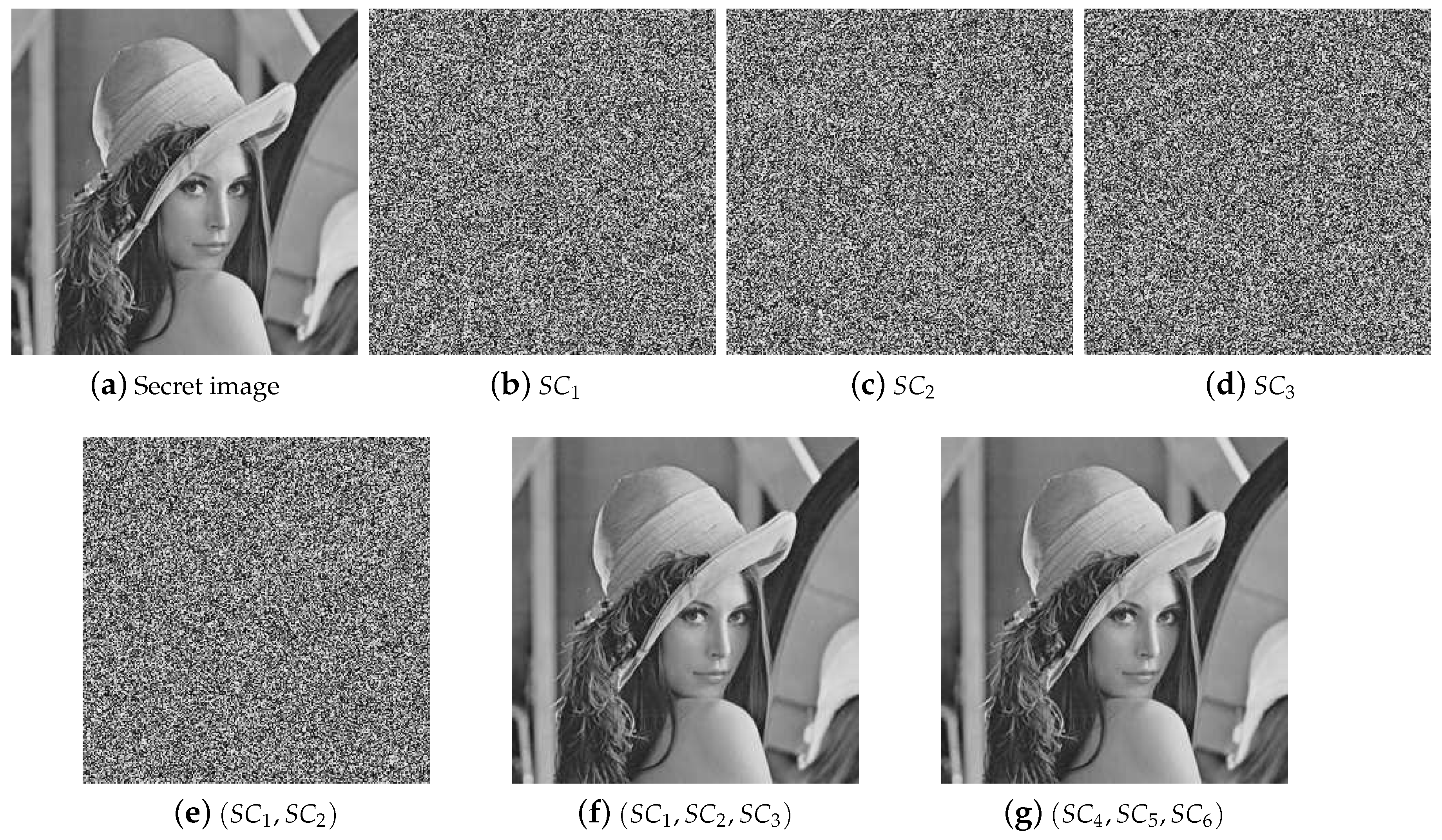
Some preliminaries are given here as the basis of our work. The goal of threshold SIS is to share the secret image S into n shadow images in such a way that: (1) knowledge of any k or more shadow images makes S easily computable; (2) knowledge of any or fewer shadow images leaves S completely undetermined.
First of all, Shamir’s polynomial-based scheme is given in
Section 2.1. Furthermore, we will introduce analysis of Shamir’s polynomial-based scheme based on matrix theory. At the end of this section, we propose the necessary and sufficient condition for
threshold SIS construction.
2.1. Shamir’s Polynomial-Based Scheme
Shamir’s scheme is based on polynomial interpolation. The scheme encrypts the secret into the constant coefficient of a random -degree polynomial in a finite field. In the recovery phase, the secret can be reconstructed by Lagrange interpolation. For example, we take a pixel value s as the gray value of the first secret pixel, and then to split s into n pixels corresponding to n shadows. The specific scheme is listed as follows:
- (1)
In the sharing phase, given a pixel value
s, we select a prime number
p, and
. In order to divide
s into pieces
, we generate a
degree polynomial
in which
and
are randomly selected in the finite field
, and then compute
and take
as a secret pair, where
i serves as an identifying index or a order lable and
serves as a shared pixel value.
The process repeats until all pixels of the secret image are processed. In the end, n shadow images are generated.
- (2)
In the recovery phase, given any k pairs , we can reconstruct by the Largrange’s interpolation, and then evaluate . Knowledge of just of these values does not suffice in order to calculate s.
2.2. Analysis of Shamir’s Polynomial Based on Matrix Theory
In Shamir’s sharing polynomial shown in Equation (
1), equations in Equation (
2) are calculated in the sharing phase. In the recovery phase, when any
k participants with
k pairs get together, the polynomial
can be reconstructed by solving the
k equations. Without loss of generality, we can assume that their pairs are
Thus, we can get
k equations as follows:
Here, the parameter
k is fixed, and
are unknown. Thus, Equation (
3) is a linear system with
k equations and
k unknowns. In another point of view, Equation (
3) is equivalent to the following vector where
deserves as a variable:
According to Equation (
4), we can rewrite Equation (
3) as Equation (
5):
Actually, linear equations in Equation (
3) and vector equation in Equation (
4) is equivalent. In addition, solution and solution vector are indiscriminate.
Using the rank of the coefficient matrix
and the augmented matrix
, we can easily discuss whether the linear system in Equation (
3) has a unique solution according to the following theorem.
Theorem 1. Assume that there is a k-variables linear equations . The necessary and sufficient condition for a unique solution is: rank(K) = rank(K,f) = k.
According to this theorem, to solve the Equation (
3) and then get the coefficients of
, we must ensure that the rank of the coefficient matrix
is
k.
In Shamir’s polynomial-based SS scheme, the coefficient matrix
of the equations is:
The coefficient matrix is a Vandermonde matrix. Because the Vandermonde matrix has a property that the rank of any
k order submatrix is
k, the equation system in Shamir’s scheme is solvable with a unique solution [
20].
One of the efficient methods to get the sharing polynomial is to use the Langrange interpolation. More generally, considering that the recovery phase is equivalent to equation solving, we can use matrix theory to solve equations and obtain the coefficients. According to Equation (
5) and Theorem 1, we can solve
through the inverse matrix of
k order submatrix.
2.3. The Design Rule of Generating the Coefficient Matrix of Sharing Polynomial
The analysis in
Section 2.2 proves that the principle of Shamir’s scheme is to select a Vandermonde matrix as the coefficient matrix to construct a polynomial and reconstruct the polynomial by Langrange interpolation.
In fact, Shamir’s sharing polynomial constructed by the Vandermonde matrix is only a special case of constructing a sharing polynomial satisfying a threshold. We can use a more general coefficient matrix to construct sharing polynomial equations, to encrypt the secret into n shares and to decrypt the secret by any k shares if and only if the coefficient matrix satisfies the following theorem:
Theorem 2 (Objective Theorem)
. Given an matrix and a vector in which and others are generated randomly, we can construct a linear system of equations to encrypt s into n shares. In the recovery phase, in order to reconstruct vector by any submatrix of and corresponding shares, must satisfy the following condition:
Any k row vectors of the coefficient matrix are linearly independent.
The correctness of this theorem is obvious. Once the coefficient
meets Theorem 2, the rank of any
k order submatrix of
is
k. According to Theorem 1, k-variables’ linear equations
in Equation (
3) has a unique solution. Hence, a coefficient matrix satisfying Theorem 2 can be applied to construct the sharing polynomial. In addition, in the recovery phase, we can decrypt the shares to secret by solving the inverse matrix instead of using Langrange interpolation. Thus, a
threshold SIS scheme could be constructed.
The question now is how to construct the coefficient matrix satisfying the requirement in Theorem 2. In the following section, we will first introduce a coefficient matrix generation approach and further propose a general threshold SIS construction based on matrix theory.
3. The Proposed Construction Method
3.1. The Basic Idea
In order to construct the SIS, we first need to construct a matrix
with size of
, which satisfies Theorem 2. Let the constructed matrix serve as the coefficient matrix shown in Equation (
4) and compute
to get shared pixel values of shadow images. The shadows are distributed to participants, and every row vector of
is distributed to corresponding participants as well.
In the recovery phase, suppose that
k participants get together to reconstruct the sharing polynomial. After the polynomial is reconstructed, the secret is obtained by
. Next, we will introduce our method and proof in
Section 3.2, and we will also do a feasibility study showed in
Section 3.3.
Section 3.4 gives a detailed construction method of the proposed general
threshold SIS scheme.
3.2. Construction Method of the Coefficient Matrix
This part will show how to construct the matrix satisfying Theorem 2. Based on the analysis, we summarize a construction method as Theorem 3. According to Theorem 3, the coefficient matrix is constructed by a special matrix , in which the determinant of all submatrices is non-zero.
Given matrix
and
, and the
k-dimensional row vectors (
) are linearly independent. For example,
can be a Vandermonde matrix. We note that
and
are generated by random assignment and validation. In addition, the feasibility analysis is given in
Section 3.3. Then, we compute
Thus, we can get another matrix
in which the
k-dimensional row vectors are linearly independent. Then, we create a new matrix
by concatenating the two matrices
and
:
and the size of matrix
is
.
That is to say, any vector
can be expressed linearly by row vectors in
. Gathering these linear expressed into a matrix form, we have
in which
serves as a temporary coefficient matrix. By computing
and concatenating
and
, we will get a matrix
which satisfies Theorem 2.
We note that the row vector group of and are all linearly independent. However, any k vectors selected between and are not apparently linearly independent, which is the reason why we give Theorem 3 and the corresponding proof.
Theorem 3 (Conditional Theorem)
. Given a set of linearly independent k-dimensional row vectors , which form a matrix Let matrix satisfy that all the minors of matrix are nonzero. Let and Thus, we can conclude that any k vectors of the coefficient matrix are linearly independent.
Proof. Select any k vectors to form . The aim is to prove that are linearly independent.
- (1)
For the case of , since the vectors of are linearly independent, the vectors of are linearly independent.
- (2)
For the case of , since and is invertible, the vectors of are linearly independent.
- (3)
For the case of
, let
, thus there are
s vectors in
and
t vectors in
are linearly independent and
. Without loss of generality, we assume that
and
in which
Consider the equation
according to Equations (
8) and (
9), we have
Since
are linearly independent, according to matrix theory, we get
which can be written as
Then, the size of
is
, and
t range from 1 to
k. Now, look at the coefficient matrix in Equation (
13) whose rank is
. Since all the minors of matrix
are full rank, the rank of
is
t, that is,
. Thus, the determinant of the coefficient matrix in Equation (
13) is nonzero. Hence, from Equation (
13), we get:
Thus, according to Equation (
10),
are linearly independent, that is to say,
are linearly independent. □
Thanks to the matrix has the special property, the matrix has such a property: any k vectors of the coefficient matrix are linearly independent. Because of that, we can construct a threshold SS ( ranges from k to ). For the purpose of simplicity, we assume a as threshold in the rest of this paper, which is enough for real applications.
Based on the constructed coefficient matrix , we will introduce a method of constructing threshold SIS schemes.
3.3. Feasibility Analysis
Generating linearly independent vectors is a difficult problem in mathematics. However, the random search method can be a solution. Estimates of the density of matrix show that one could easily find the initial matrix and the temporary matrix satisfying Theorem 3.
Randomly select
n vectors in a set
; the probability of these vectors being linearly independent is
:
For example, when . Thus, when p is a big prime number, the probability of any n vectors being linearly independent is very high. That is to say, the initial matrix of which the vectors are linearly independent is easily to be generated.
Furthermore, when taking into consideration that all the minors of an
are nonzero, we can analyze the probability by way of the method mentioned above. Let
be the probability of that all the
minors of
(
i range from 1 to
n)are nonzero. Hence, we get:
Thus, we can get the value of
, the probability of that any minors of matrix
is nonzero, as follows:
When
,
which implies that we need average every
times to get such a matrix
that satisfies our Theorem 3.
Thus, we can get randomly generate a qualified matrix by average 40.58 times. This implies that the construction is feasible.
3.4. The Algorithms of Secret Image Sharing
At the beginning of this section, we first connect the theorems to each other. Theorem 1 is the necessary and sufficient condition that the linear equations have a unique solution. The objective theorem Theorem 2 is the principle that must satisfy according to Theorem 1. The conditional theorem, Theorem 3, is the method of constructing coefficient matrix to satisfy our objective theorem. Hence, we could get a general threshold SIS construction.
In this section, we use the constructed coefficient matrix to achieve polynomial-based SIS. In what follows, the original grayscale secret image is represented by S, and the size is Without loss of generality, we split the first secret pixel s into n pixels corresponding to n shadows’ images.
3.4.1. The Sharing Phase
In the sharing phase, to divide the secret
s into pieces
, we generate a matrix
constructed by the way mentioned in
Section 3.2. We select a prime number
p. We generate a vector
where
and the others are
random integer numbers generated in the finite field
. Then, compute
as follows:
is distributed to the ith participant, as well as the corresponding ith row vector of the matrix . We take as a share, where serves as an identifying index or a key and serves as a pixel value. The steps are described in Algorithm 1.
| Algorithm 1. The proposed general threshold SIS construction by matrix theory for sharing phase |
Input: The threshold parameters (, a matrix constructed by Theorem 3, a secret image S with size of and a prime number p
Output: n shadow images |
Step 1: For every secret pixel s in each position , repeat Step 2–3.
Step 2: Generate a vector , set , and generate others randomly in the finite domain .
Step 3: Compute , where .
Step 3: Output n shadow images |
The pseudo code of Algorithm 1 is presented as follows:
| Algorithm 1 Matrix |
- 1:
for to M do - 2:
for to N do - 3:
- 4:
generate randomly - 5:
- 6:
for to n do - 7:
- 8:
end for - 9:
end for - 10:
end for
|
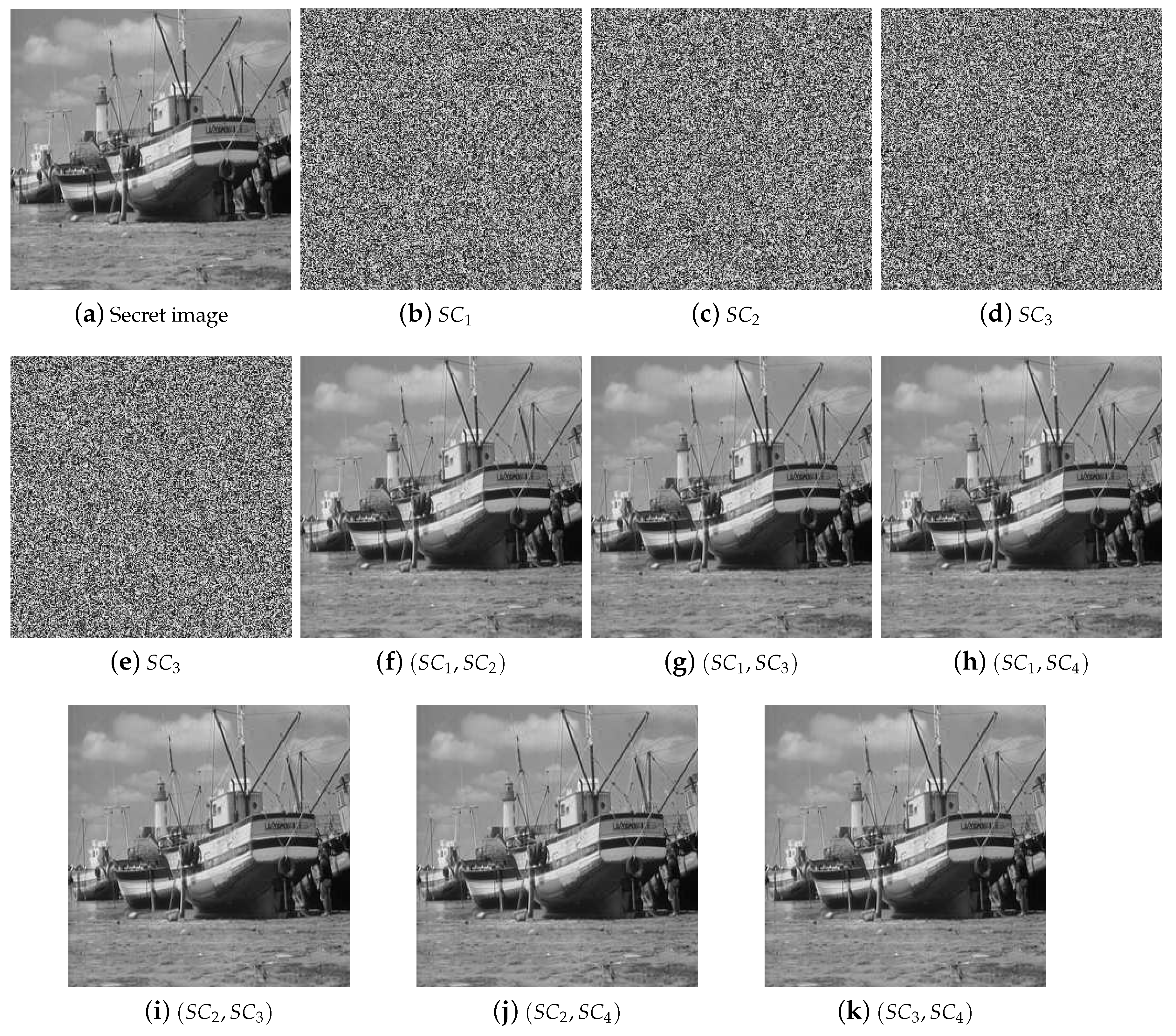
Finally, according to Algorithm 1, the n shadow images are generated succesfully by the proposed SIS scheme based on matrix theory. It should be noted that we utilize the largest prime number less than 255; however, the grayscale pixel value of an image ranges from 0 to 256, so our construction is not totally lossless. However, it is still a high resolution SIS construction method.
3.4.2. The Recovery Phase
In the recovery phase, given any
k pairs
, we can concatenate
k vectors
to generate a submatrix
. Thus, we can finally obtain the vector
by solving the following linear equation:
the secret pixel
s is the value of
. Note that all the calculations are performed in a finite field. The value of
will not be solved if the number of linearly independent vectors is less than k. The specific recovery steps are shown in Algorithm 2.
| Algorithm 2. The proposed general threshold SIS construction in matrix method in recovery phase |
Input: The k shadow images which are randomly selected from n secret shadow images and corresponding k vectors
Output:The original secret image S |
Step 1: According to the k vectors , concatenate k vectors to a matrix .
Step 2: For each position , repeat Step 3–4.
Step 3: According to the Equation (4), construct linear system.
Step 4: Get the coefficient of by computing linear system according to Equation (19), and set the pixel .
Step 5: Output the secret image S. |
The pseudo code of Algorithm 2 is presented as follows.
| Algorithm 2 recover |
- 1:
for to M do - 2:
for to N do - 3:
for to k do - 4:
- 5:
- 6:
- 7:
- 8:
end for - 9:
end for - 10:
end for
|
3.5. Complexity Evaluation
The algorithm complexity for decryption of Shamir’s scheme is , while k is the total number of shares participating in recovery. In addition, the algorithm complexity for equation system solution is . Since the coefficient matrix is not a sparse matrix, the algorithm complexity of the proposed method is , which is a little higher than that of Shamir.

