1. Introduction
The analysis of micro-circuitry is an indispensable foundation in neurobiological research. However, the anatomical connection linking the function of the brain in the nervous system is still poorly understood [
1,
2]. Electron Microscopy (EM) is a strong acquisition technique for reconstructing connectivity between neurons because it can provide high resolution that enables us to identify the synapses possible [
3]. Unfortunately, the complexity of these images makes it a labor-intensive enterprise requiring an impractical amount of time on manual labeling. Therefore, automatic reconstruction methods are in high demand [
4].
The first step of neuronal circuit reconstruction focuses on detecting neuron membranes, which is also treated as neuron segmentation task. These boundaries can help distinguish individual neurons that are essential to form a complete neuron [
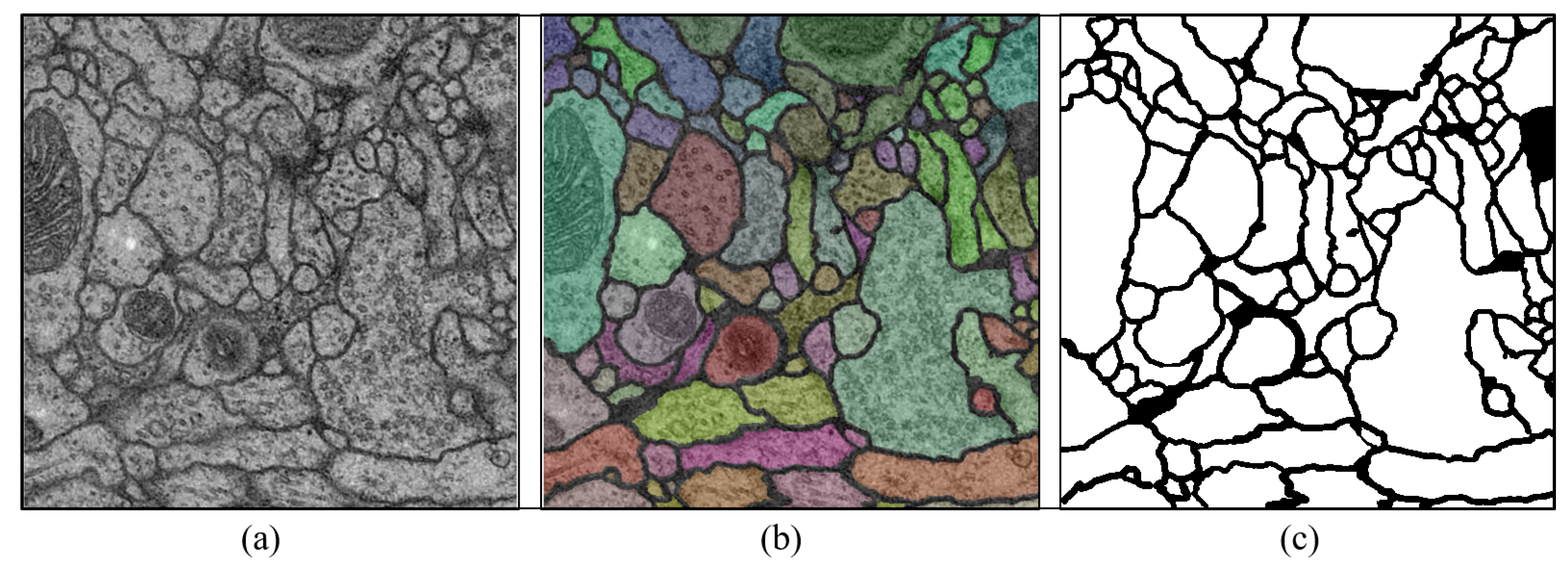
5]. A two-dimensional example is illustrated in
Figure 1: raw EM image, its corresponding segmentation result (individual neurons are labeled in different colors) and neuron membrane detection result. The task poses a difficult challenge, due to several issues: (1) the complex intracellular structure makes it difficult to identify the neuron membrane, (2) local noise and ambiguity caused by imperfections in the staining and imaging may blur the membrane boundary, and (3) the physical topologies of cells have large variations, especially in the thickness [
3,
5,
6,
7].
Recently, many methods have been adopted to tackle this problem. The majority of neuron membrane segmentations heavily rely on deep learning. Early approaches [
8] used deep neural network to predict each pixel in a fixed window which dramatically limits the contextual information. For this reason, researchers sought to find a more efficient and scalable deep neuron network in such segmentation task. Fully convolutional network (FCN) [
9] and its variants have gained much attention [
10,
11], using encoding and decoding phases for the end-to-end semantic segmentation. Besides, they use residual connections in order to increase network depth to gather more contextual information [
12,
13,
14]. The defects of these CNN-based segmentation methods are obvious: on one hand, the receptive field is always limited due to inflexible kernels of convolution layers [
15]; on the other hand, most of these existing methods only employ the traditional pixel-wise loss (e.g., SoftMax) to optimize the model with certain disadvantages, such as image blur and sensitivity to outliers due to insufficient learning of local and global contextual relations between pixels [
16].
To address these problems, we propose our adversarial and densely dilated network (ADDN) inspired by the power of conditional Generative Adversarial Network (cGAN) in image translation [
17,
18]. For one thing, a fully connected CNN in generation network, which is known as “Segmentor”, is applied to provide the segmentation result. Without using a particular task-specific loss function, we specify a high-level goal for the network to produce realistic images that are indistinguishable for the “Discriminator” from the ground truth. In this case, blurry images will be avoided with the adversarial training loss. For another, without using the basic encoder-decoder network as the “Segmentor” unit, we propose an extension of U-Net [
11] by using dilated dense blocks [
19,
20,
21] in each level of the network with skip connections to make the entire network extend its perceptual regions with limited trainable weights as well as convolutional layers. Furthermore, dense connections have a regularizing effect, which reduces overfitting on this EM image segmentation task with small training set sizes [
20].
Overall, (a) to overcome the limitation of receptive fields, we carefully design our segmentor with dense connection and dilated network based on U-Net architecture. The U-shape structure is flexible and can capture low-level and high-level information via skip connections. Besides, auxiliary dense connection and dilated network further enlarge the receptive fields without adding any training burdens. Therefore, our network makes full use of the contextual information. (b) To overcome the local objective problem, our GAN-based model utilizes the adversarial training instead of single traditional loss which sets a high-level goal and greatly promotes the segmentation performance. We evaluate our method on two publicly available EM segmentation datasets: ISBI 2012 EM segmentation challenge and mouse piriform cortex EM dataset. Our model tends to achieve comparable accuracy to other state-of-the-art EM segmentation methods but requiring much fewer parameters than existing algorithms. The main contributions of our work are as follows:
As far as we know, adversarial neural network is at the first time applied to connectomes segmentation with EM images. The adversarial training approach enhances the performance without adding any complexity to the model used at test time.
For connectomes segmentation problem, we combine U-Net architecture with dilated dense block which takes the advantage of dense connection and dilated network. Compared with other U-net-based models, it enlarges the receptive fields and saves computation expenses.
In contrast to the classic GAN with a single loss function, we combine the GAN objective with the dice loss for alleviating the blurry effects. Therefore, the tasks of the segmentor are to fool the discriminator as well as to generate more accurate images.
The ADDN is an end-to-end architecture trained and with can achieve favorable results without further smoothing or post-processing. We demonstrate that ADDN performs greatly by comparing the state-of-the-art EM segmentation methods on two benchmark datasets.
The rest of the paper is organized as follows. The related work will be introduced in
Section 2.
Section 3 describes our ADDN architecture and methodology. In
Section 4, the associated experiments as well as the obtained results are described in detail. Finally,
Section 6 concludes the paper.
2. Related Work
Image segmentation. In the field of computer vision, image segmentation is the process of segmenting a digital image into multiple image sub-regions based on position, color, brightness, texture, etc. One popular method for image segmentation is level set method (LSM) introduced by Osher et al. [
22] which can track interfaces and shapes without parameterizing the object. Particularly, it has been widely used to overcome the difficulty of image intensity inhomogeneities [
23,
24].
Another problem in image segmentation is that segmenting every pixel is harder due to growing size of images and computational expenses. Superpixels [
25] are a collection of perceptually similar pixels sharing low-level image properties which is beneficial for extracting local features and representing structural information. Therefore, it greatly reduced representational and computational complexities and was applied to many different fields. There are many available superpixel segmentation algorithms. For example, the basic idea of the classical watershed algorithm [
26,
27] is to construct a watershed to divide the different collection basins from the local minimum of the image along the gradient ascent. Although the algorithm is fast, the severe over-segmentation makes it less efficient. Levinshtein et al. [
28] proposed Turbopixel algorithm. In order to make superpixels regularly distributed, the image is segmented into meshed superpixels by progressively expanding the seed point using geometric-flow-based LSM. It is also good for its speed but its edge fits undesirably.
Connectomes segmentation. Several authors have contributed to the neuron boundaries detection problem for direct reconstruction from EM data. Earlier works focus more on interactive membrane delineation in 2D EM images [
29,
30], which are involved with too much experts’ knowledge. More recent works [
3,
5,
6,
31] rely on machine learning techniques for automatic membrane detection. For example, in [
31], the random forest classifier was proposed with geometrical consistency constraints. In [
5], neural networks were carefully trained using certain feature vector which was the image intensities filtered through a stencil neighborhood.
Currently, deep learning methods have shown their advantages on automatic segmentation. For EM segmentation, Ciresan et al. [
8] firstly trained a deep convolutional neural network as a pixel classifier, which decided pixel values in a square window centered on it. The method preserved 2D information and high-level features well and it won the 2012 ISBI EM segmentation challenge by a large margin. Recently, medical image segmentation approaches have been based on FCN [
9,
32] that is an effective approach to generate dense predictions. Chen et al. [
10] proposed a deep contextual network, a variant of FCN, by leveraging multi-level contextual information from the deep hierarchical structure. Ronneberger et al. [
11] modified and extended the FCN architecture by adding successive layers to a usual contracting network. The contracting path aimed to explore contextual information meanwhile the symmetric expending path enabled precise localization. Residual connection [
33] demonstrates its efficiency in image classification task. These shortcut connections have been applied to segmentation areas [
12,
13,
14]. Quan et al. [
12] leveraged the summation-based skip connections to allow a much deeper network architecture than [
11]. Similarly, in [
13], Michal et al. extended Residual Network to FCN for semantic image segmentation of hundreds of layers. Ahmed et al. [
14] proposed residual deconvolutional neuron network which was formed with similar informative paths for fully extracting image features. Detailed comparisons of each method can be seen in
Table 1.
Overall, most of these deep learning-based methods are for the purpose of obtaining more contextual information with minimum additional computation. Despite of the abovementioned algorithms, EM image segmentation problem still contains much for improvement. For this reason, we introduce adversarial training in our work. Many recent methods have achieved state-of-the-art accuracy by employing GANs. GANs have a critic network optimized to distinguish real images from fake ones such that the generator network will be motivated to synthesize more realistic images. Similar adversarial training approaches have been explored in different academic fields, such as text-to-image translation [
35], image-to-image translation [
17], single image super-resolution [
36] and image segmentation [
37]. Applying similar segmentation to medical imaging is popular e.g., segmentation for brain MRI [
38,
39], organs in chest X-rays [
40], and prostate cancer MRI [
41].
In the paper, we propose a new connectomes segmentation network using adversarial training to enhance segmentation outcomes inspired by conditional GAN [
42] which is an extension of traditional GAN model. In contrast to aforementioned work, we design a U-Net based network as our segmentor whose convolutional layers are replaced by dilated dense blocks to achieve more contextual information.
3. Proposed Method
Given the special challenges of EM image segmentation problem, we design the network based on the experimental results and best practices. In this section, we start with explaining the general design of our ADDN model. Then, the detailed architecture of each component is elaborated.
3.1. Overview
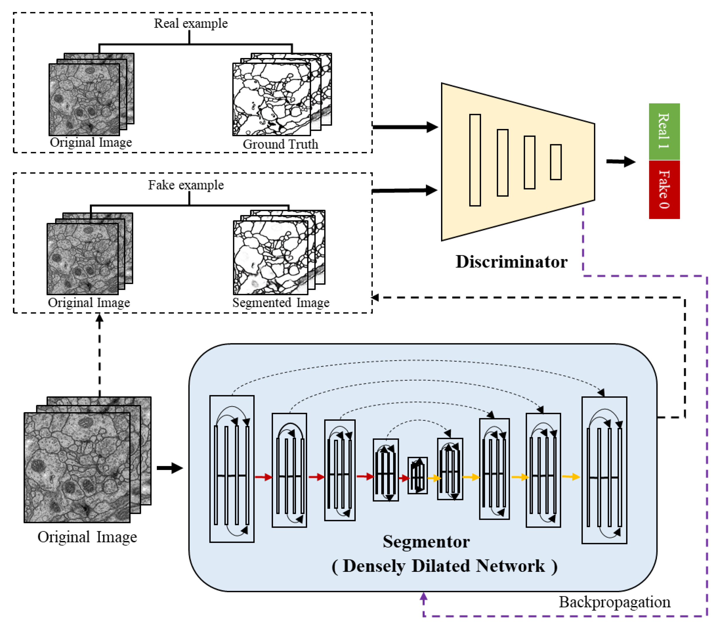
Figure 2 shows the overall architecture of the proposed ADDN which consists of segmentor and discriminator network. Typically, the segmentor is composed with encoders and decoders network. To tailor to the connectomes segmentation problem, the standard convolution layers in the network are replaced by dilated dense blocks. It is similar to the generator in traditional GANs which produces a probability label map, while conditioned on the input image. The discriminator takes the ground truth label maps or predicted label maps along with original EM images as input. It is trained to discriminate the synthetic labels from ground truth labels meanwhile making them as similar as possible. These two networks can be trained jointly through optimizing the segmentor and discriminator in turn.
3.2. Training Objectives
We firstly define as segmentor and discriminator network. The data contains input image x and its corresponding ground truth y. The size of x is where H and W are for image height and width respectively, and single channel means grayscale. Accordingly, y is which has the same image size and C different classes. We use , to denote input and ground truth value at pixel position of i. denotes the class probability predicted by S.
The cGAN in this case defines the optimization problem as follows:
where
x is not only the input image which replaces random noise in traditional generator network, but also the observed image.
S tries to minimize this objective while an adversarial
D tries to maximize it.
Previous work [
17] has demonstrated that combining cGAN loss with a more traditional loss is effective for encouraging less blurring. Given our segmentation task, we add an additional dice loss in our proposed method. Therefore, our objective is
where the dice loss is
Here,
is a constant value which means the weight for balancing two losses. We can solve Equation (
2) by alternatively optimizing between
S and
D via using their respective loss functions.
Training discriminator network. The inputs of the discriminator network interactively switch between
and
during training:
denotes the concatenation of the annotation and the input, and
denotes that of the segmented map and the input. The loss function of the discriminator
is composed of two binary cross-entropy losses and its calculation formula as follows:
where
The discriminator is trained by minimizing and when concerning D, the S is fixed.
Training segmentor network. The loss function of the segmentor is composed of dice loss and the adversarial loss. In particular, given certain
D, the segmentor is trained by minimizing the loss function:
Only the is related to gradient, therefore, it is engaged in the first loss term .
3.3. Segmentation Network
We use a DDN which is an adaptation of DenseNet for semantic segmentation [
21]. The architecture has an encoder-decoder structure including downsampling path and upsampling path. In
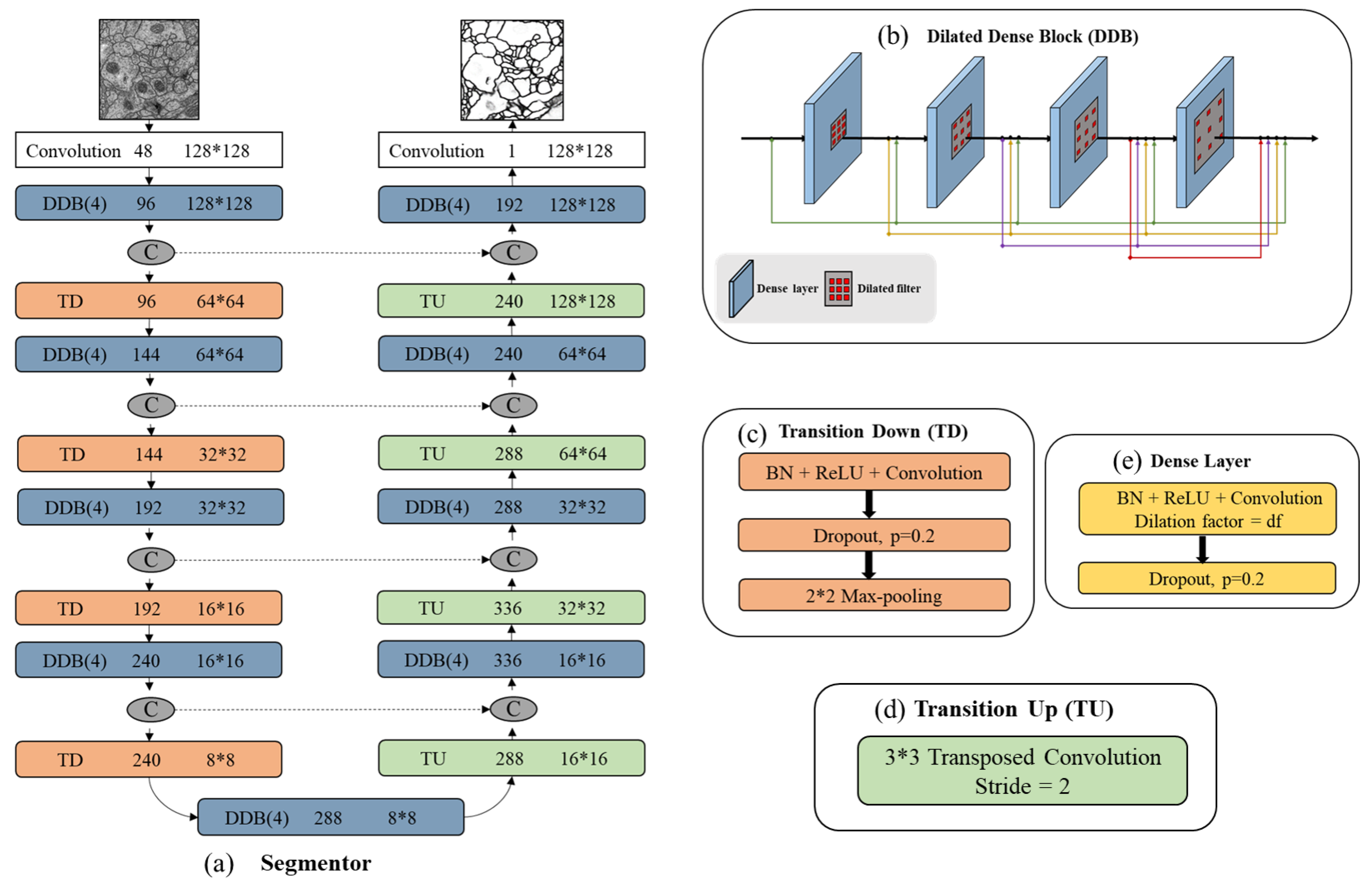
Figure 2, the red lines are the downsampling path which recovers the abstract image representing by gradually reducing spatial resolution and increasing semantic dimensionality. The yellow lines are the upsampling path aiming at predicting pixel-level class probabilities. Besides, we follow the design of U-Net by adding the skip connections to share the low-level information between input and output (e.g., boundary information). The black dashed lines in segmentor are such skip connections that help capture context and local features simultaneously. The segmentor architecture (see in
Figure 3) has three main blocks: dilated dense block (b), transition down (c) and transition up (d). A dilated dense block (DDB) has four dense layers (e). Each dense layer is formed with BN, ReLu, dilated convolutional layer and dropout layer. Here, ReLu is our activation function, the learning rate is set as 0.2. In particular, the BN and dropout layer are added to reduce over-fitting during training. Transition Down (TD) contains one dense layer and an additional max pooling layer. Transition Up (TU) modules have a transposed convolution to upsample the previous feature maps.
Notice that DDBs are adopted as the core module in the segmentation network. For one thing, we use dense connection in this block. Formally, assume
is the output of the
lth layer,
is the convolution function and it can be computed by:
The reason to use dense connection lies in that it can alleviate the effect of vanishing gradients. It overcomes the difficulty of gradient propagation through lower layers in the network. It can also maximize information flow because the input of each layer consists of feature maps output from all preceding layers. For another, we utilize dilated convolutions, which help the layer weights sparsely distributed so that enlarging the receptive fields. Proper dilation factor helps capture wider context information.
In
Figure 3a we summarize all segmentor network layers. This structure is built from a first convolution layer on the input, four DDBs and four TDs in the downsampling path, one DDB in bottleneck (last layer of the downsampling path), four DDBs as well as four TDs in the upsampling path. The number of feature maps produced by each dense layer is called growth rate which is defined as parameter
k and is set to 16. If not otherwise mentioned, every convolution has a kernel size of
and each DDB has the dilation factor of {1,2,4,8}. Skip connections are between mirror-symmetry convolutional and deconvolutional layers which are not shown in the figure.
3.4. Discriminator Network
Our discriminator structure is illustrated in
Figure 4. It is designed for differentiating between the segmented images and ground truth to further refine segmentation results. Therefore the input is the concatenated pairs of original EM images and estimated segmentation or manual segmentation images. Note that, the PatchGAN [
17] is used in this architecture as the classifier, which tries to distinguish if the image is natural or generated through such
patch.
In
Table 2, it shows the configuration of discriminator network in detail. Four convolution layers along with batch normalization layers and LeakyReLU activation layers (except for the last layer) act as the feature extractor. In this case, there are no pooling layers used in discriminator, instead, images are downsampled using convolution layers with stride 2. The sigmoid function is stacked at the end of these convolution layers to regress a probability score of each pixel ranging from 0.0 to 1.0. If the value is close to 1.0, the input is real otherwise is fake. The patch size is set to
.
3.5. Evaluation Metric
For evaluating segmentation quality, we adopt the standard metric maximal foreground-restricted rand score after thinning (
) described in [
43]. We assume
S to be the segmentation result and
T be the annotated images. Here
denotes the joint probability that a pixel belongs to segment
i in
S and segment
j in
T.
Foreground-restricted Rand F-score is the most frequently used for such datasets and it is also introduced by the official ranking system that weights
and
equally.
3.6. Implementation Detail
In our experiment, we pre-train the segmentor via dice loss because it is beneficial for training GANs and greatly accelerating the procedure. All the convolution layers were initialized with HeUniform [
44]. We randomly cropped a region of
from the original images as the input and used Adam optimizer with an initial learning rate of 0.0002 to optimize the objective function. The model is trained for 100 epochs with mini-batch size 2. When training involves discriminator, in order to slow down its speed, we perform two optimization steps on the segmentor and one step on discriminator in one batch. We implemented the model in Keras [
45] with NVIDIA GTX 1080 GPU.
4. Experiment
In this section, we employ relative experiments to testify the effectiveness of our model on two EM image datasets.
4.1. Datasets
ISBI 2012 EM segmentation dataset. The dataset is from ISBI 2012 EM segmentation challenge [
43] which is still open for new contribution. For training, the provided set contains a stack of 30 grayscale slices collected from
Drosophila first instar larva ventral nerve cord (VNC) which is through the new techniques ssTEM. For testing, another set of 30 images is included while segmentations are held out by the organizers for evaluation.
Mouse piriform cortex dataset. The datasets are assembled from the piriform cortex of an adult mouse prepared with aldehyde fixation and reduced osmium staining [
46]. The 2D EM images are assembled into 3D stacks (total 4 stacks) and manually annotated. In our experiment, we use stack 2, 3, 4 for training and stack 1 for testing.
4.2. Data Augmentation
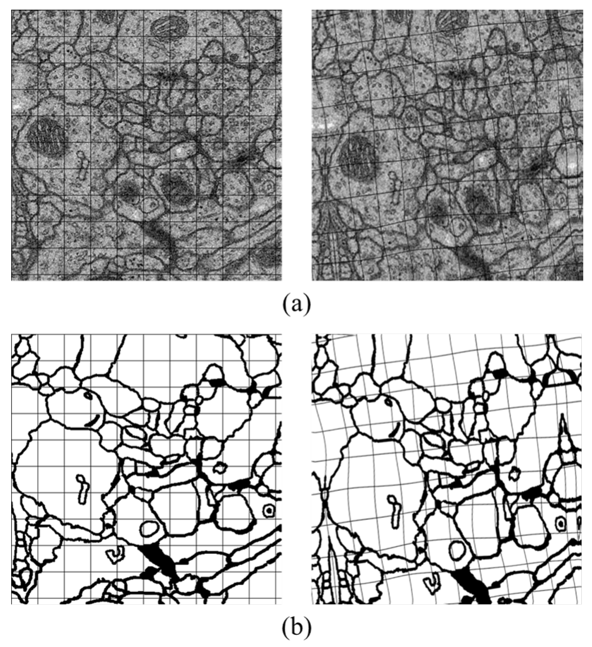
Data augmentation is a practical method which is aimed at generating more useful data during the deep neuron network training. Therefore, we utilize it to enrich our data by forming about 10 times larger of the raw images and their labels. There are two simple approaches in our experiments for transformation including rotation by four different angles () and flipping with different axes (up-down, left-right, no-flip). We also adopt elastic distortion which is suitable for EM images and thus with no requirements of other complex deformations.
Elastic distortion. It is a commonly used strategy in machine learning to enrich dataset, with the ability of emulating some autonomous biological conditions [
47], e.g., uncontrolled oscillations of hand muscles in handwritten digit recognition task. Elastic distortion applies a displacement field to the target image, which is built by convolving a randomly initialized field with a Gaussian kernel. Then, the field is interpolated to the original size of the image, and forms the new one.
Figure 5 is the example of the transformation. Slight distortion can be seen in the figure, which is coincident with the variation of cells physical topology.
4.3. Ablation Study
To explore the effectiveness of different modules, we perform the following ablation studies. Note that, in our experiment, we take use of 30 images in ISBI 2012 EM training set by splitting into 24 training images and 6 validation images. For mouse piriform cortex dataset, we preserve parts of the images and use stack 2 for training and stack 3 for validation. Validation set is utilized to demonstrate the performance of adversarial training as well as our DDBs in segmentor network, then tune our hyperparameters to select our final model.
4.3.1. The Effectiveness of Adversarial Training
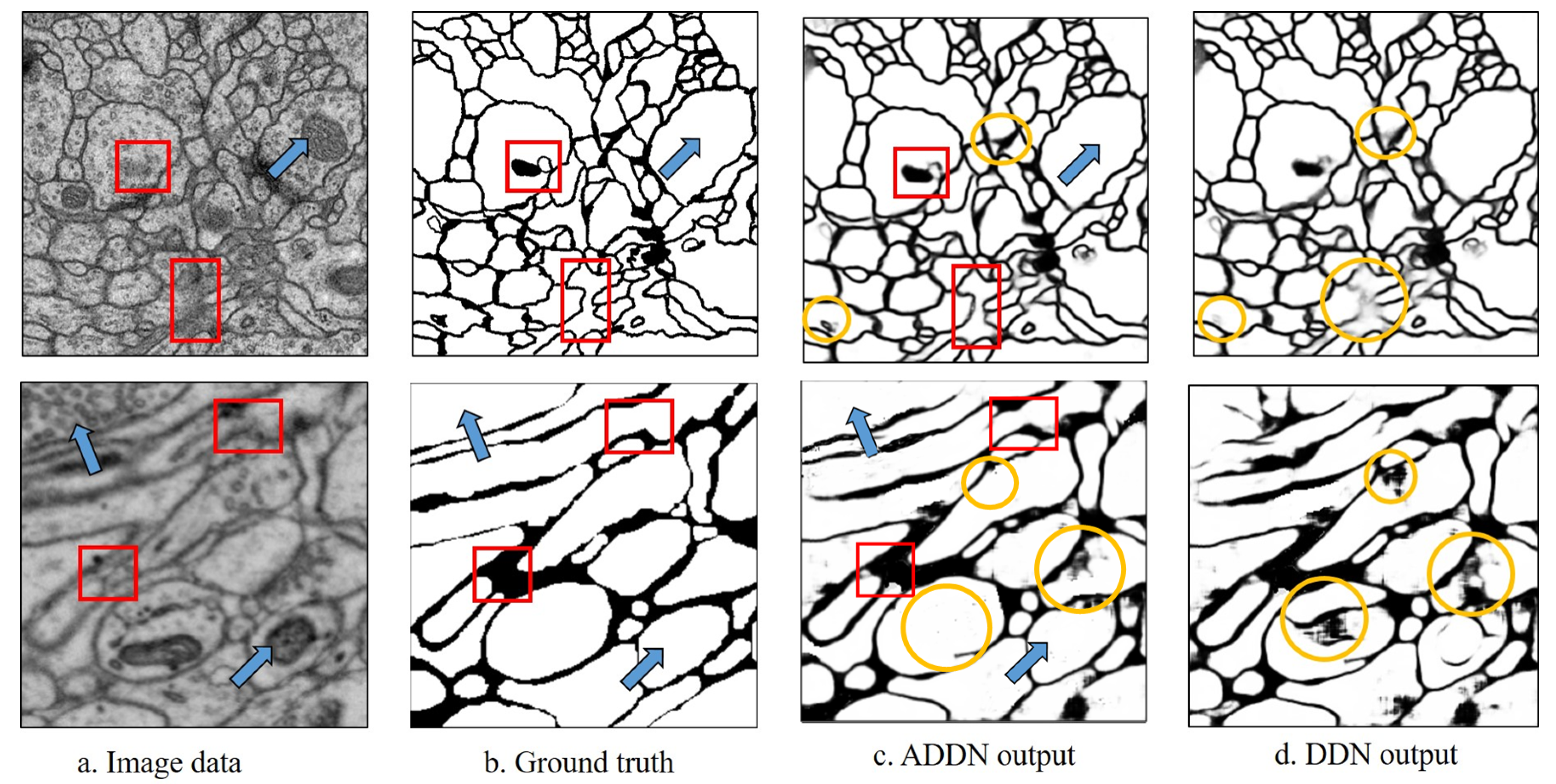
To verify the importance of adversarial training, we compare our proposed ADDN with DDN. Here, DDN is the segmentor network without adversarial training thus the training objective is only to minimize the dice loss for connectomes segmentation.
The experimental results are shown in
Figure 6. As the yellow circles show, borders appear fuzzy in DDN without adversarial training. It well demonstrates that with adversarial training, the segmented images are less blurry. Overall, ADDN produces a more accurate segmented image.
Then, we conduct further experiments to exploit the best loss function yielding to better performance during adversarial training. We train four different models: densely dilated network which is treated as the baseline, densely dilated network with only cGAN loss (DDN+cGAN), densely dilated network with both cGAN loss and L1 loss which is a more traditional loss in computer vision (DDN+cGAN+L1) and ADDN with both cGAN loss and dice loss. As shown in
Table 3, the best result is in bold which is similarly applied in the following tables. cGAN loss together with dice loss achieves the best rand score. L1 loss seems to make little difference in this task and single cGAN loss is not sufficient to boost the segmentation result.
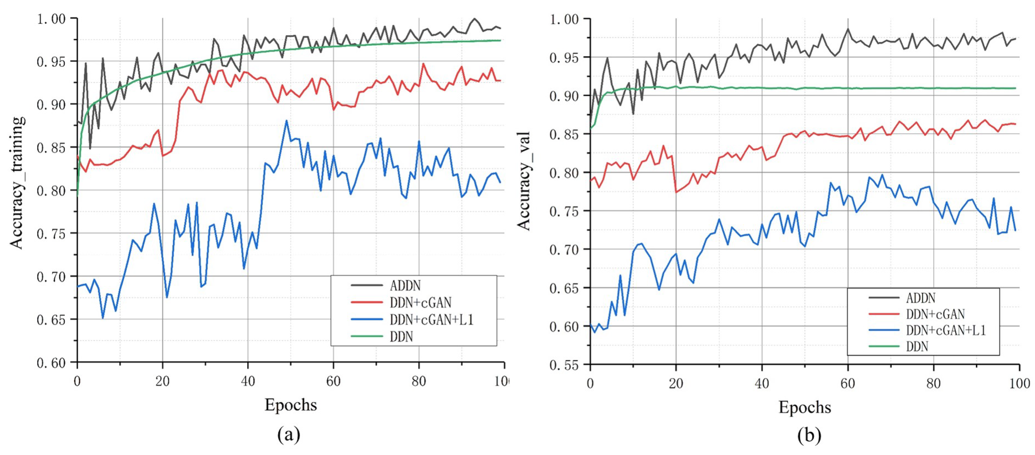
To further explore the performance of different losses, we analyze their training accuracy in
Figure 7. We can find out that no matter training or validation, DDN has the best training efficiency. Comparing GAN-based models, training with cGAN loss or both cGAN and L1 loss are less stable than ADDN and their training efficiency is almost similar.
4.3.2. The Effectiveness of Proposed Segmentor Network
As mentioned in the previous section, we design our segmentor network in order to refine our segmentation result by capturing more contextual information during training. The evaluation is performed on some baseline models where the segmentor networks are all the variants of U-Net architecture. The discriminator and training loss keep the same, while the segmentor networks are divided: U-Net architecture(AUN), Dense-U-Net architecture (ADN), Res-U-Net architecture (ARN), dilated FCN (ADFN) and our ADDN.
First, for training AUN, we replace the DDBs in segmentor with standard convolution layers with 64, 128, 256 and 512 filters as in [
17], which is commonly used in relative fields. Then, we use residual blocks in ARN where convolution layers are connected with residual connection. For ADFN, we follow the design of [
38] which consists of 16-layer FCN and dilated network. Finally, we additionally train the ADN without dilation to explore the effect of dilated network. The achieved rand scores are described in
Table 4.
The comparison of all the networks demonstrates that our proposed segmentor is able to obtain the highest rand score in both two datasets. Besides, comparing AUN, ARN and ADN, we can find that convolution with dense connection achieves more favorable segmentation results than that with residual connection and only traditional convolution. We also can find that FCN structure is relatively too coarse to achieve good results in this case. Furthermore, the comparison of ADN and ADDN verifies the effectiveness of dilated convolution.
By analyzing
Table 5, we can obtain the computation expenses of all the networks. It can be observed that our proposed architecture uses the least parameters. It is only 8.9 M, almost 12 times less than ADFN, 7 times less than ARN and 5 times less than AUN.
4.3.3. Hyperparameter Study
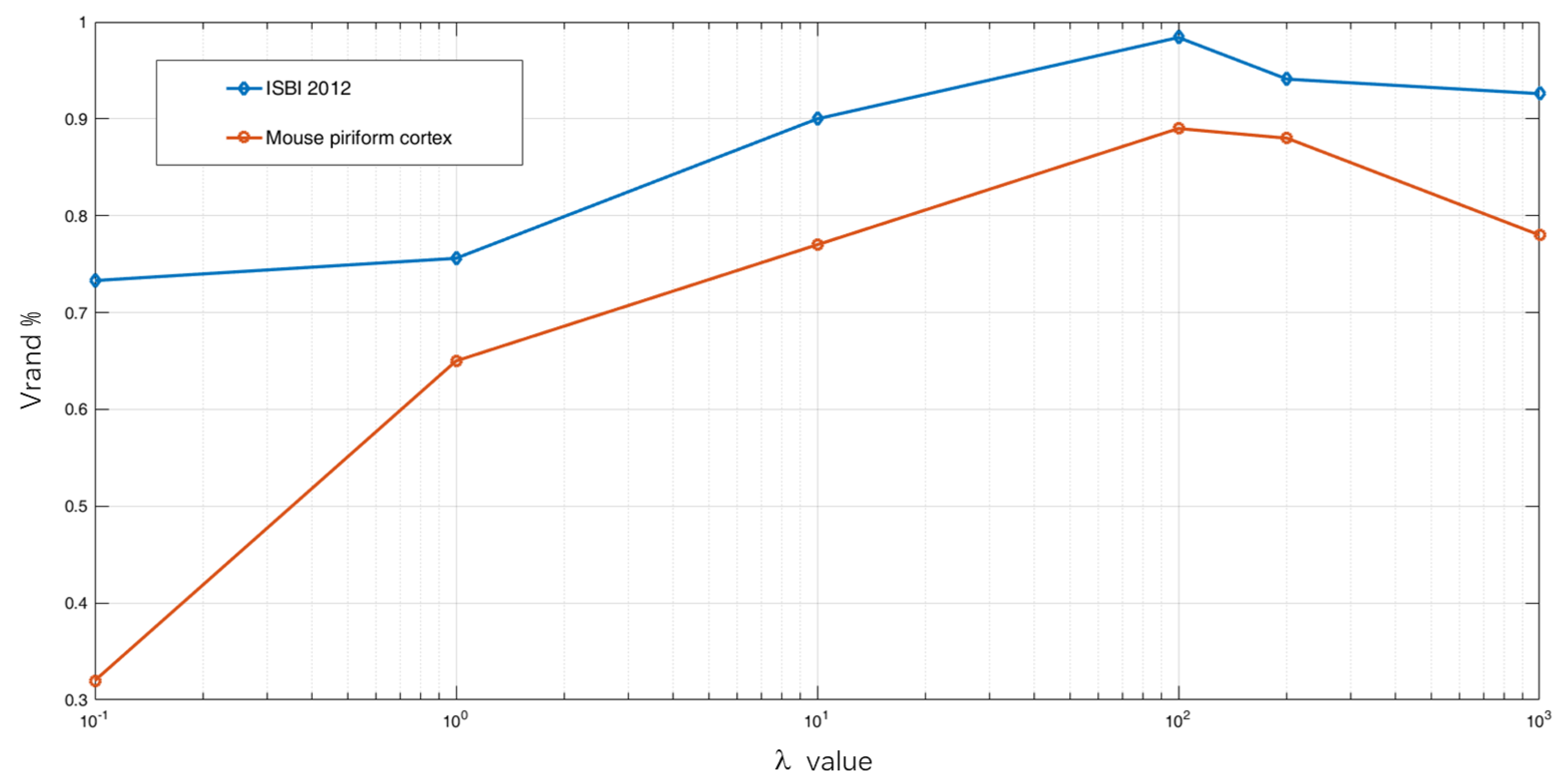
Selection of . is the hyperparameter in Equation (
6). In order to choose the optimum value, comparable experiments have been performed on two datasets. As shown in
Figure 8, we find that the best rand score is obtained at
.
rises rapidly because the weight of dice loss becomes more significant compared to
loss. However, when it far outweighs
loss, the rand score decreases instead. Thus, we empirically assign 100 to
in our following experiments.
Selection of growth rate. The growth rate
is an important parameter for densely connected networks which decides the amount of passing information of each layer. Theoretically [
20], growth rate is with no requirements to be too large thus we compare four different values using ISBI 2012 training and validation set and all the results are obtained by averaging 5 results in ISIB 2012 validation set. As shown in
Table 6, with
k increasing, the rand score is higher however it is limited by consumption of GPU memory (when
). Therefore, in our final model, we utilize 16 as our growth rate.
4.4. Performance Comparison
Qualitative comparison.Figure 6 demonstrates the qualitative results of two datasets without boundary refinement. Pixels with darker color denote higher probability of being membrane. Our ADDN can identify the complex intracellular structures and accurately remove mitochondria or vesicles shown by blue arrows. The red boxes are the regions where the contrast of membrane is low, however by gaining more contextual information, our ADDN architecture is relatively robust to such image noise and successfully predicts accurate probability map. The proposed methods well tackle the previously mentioned problems.
Quantitative comparison. We compare our model with several state-of-the-art approaches on two benchmarks. Quantitative results are summarized in
Table 7 and
Table 8.
In
Table 7, we firstly evaluate the performance of our ADDN by comparing with existing published entries on ISBI 2012 EM dataset. The performance of different submitted methods will be reported on the leader board. Besides, for fair comparisons, we employ some approaches under the same conditions with ours: the same training data with same augmentation methods, the same testing data and all results without any post-processing. We can see from the table that we surpass all the deep learning methods and achieve 0.9832 rand score without any post-processing methods. From the second column, many approaches with high ranking rely on post-processing to boost their performance, such FusionNet [
12] used 2D median filter for each slice, CUMedVision [
10] used watershed algorithm and averaged 6 trained model to improve the results. That can also be seen in the third column. We find that FusionNet and U-net [
11] perform worse which may be caused by lacking post-processing. However M2FCN [
48] achieves better result in our environment which is most likely due to our augmentation methods.
Table 8 indicates comparisons on mouse piriform cortex dataset. Our model can process image of arbitrary size. However the images of this dataset have different resolutions in different stacks. Therefore, we still pick
from original images and use them to train our networks. We use the same stack for testing as [
46,
48]. And we still compare some experiments in our environment. We can observe that our approach gains higher result when comparing with other state-of-the-art models which are mostly recursive-based model. Besides, VD2D3D [
46] took a 2D convolutional network followed by a 3D network to segment. Our model only takes 2D context information while even has higher rand score than the 3D method.
5. Discussion
ADDN is proposed with novelty to overcome connectomes segmentation challenges of EM images. The approach achieves accurate segmentation performance by utilizing adversarial training which sets a high-level goal instead of traditional segmentation objectives. In this min-max game, the segmentor will struggle to improve its segmentation ability under the simulating of the discriminator. With the popularity of GANs, some studies have the similar concept with us. Dai et al. [
40] proposes SCAN architecture for chest X-ray organ segmentation problem utilizing adversarial training and residual connections. The main difference of us is that it is based on ordinary GAN which may frequently incur ill-posed problems but our model is on cGAN that is specifically designed to solve that. Moeskops et al. [
38] has the same cGAN framework and dilated network with us however the segmentor network architecture and loss function definition are quite different. Firstly, dilated FCN is a coarse architecture without skip connection or only with shallow networks thus not fully capturing contextual information. The experimental result in
Table 4 verifies that its segmentor network (dilated FCN) is not powerful and performs worst among all methods. DDN has larger receptive fields and gains more context so that the result is best. Secondly, its cGAN loss and another loss are actually separated during training while we combine them together and add a hyperparameter
as the weight sum to increase or decrease the effect of dice loss which can make the objective more flexible. To sum up, our architecture is based on cGAN framework but also special in designing segmentor network, designing objective function.
In
Table 7 and
Table 8, we have compared with existing methods in connectomes segmentation field. According to the final rand score in testing image, we outperform all the mentioned approaches. Then we further analyze them in theory. For FusionNet [
12], CUMedVision [
10] and U-Net [
11], the three methods utilize certain techniques such as residual connections, multi-level features fusion or skip connections to increase the network depth and receptive fields while it is not thorough enough due to the limitation of training ability and improper information flow. Therefore they all need the help of post-processing. For PolyMTL [
34], it bounds two FCNs together, one as pre-processor for normalizing images and the other is for segmenting. The structure is not so convenient meanwhile the pre-processor contributes too much and makes the segmentation network less effective. For M2FCN [
48], the main defect is that dealing with sequential input is time-consuming and heavily increases computational expenses. Compared with them, our architecture takes the advantage of dense connection which has proved superior than residual connection and simple convolution, and dilated network to avoid the training burden and to gain more contextual information. Besides, it is trained end-to-end with arbitrary input size and when testing, only segmentor network will be involved. It is more convenient than PolyMTL. Moreover, it considerably saves its computational expenses.
There are still some limitations of our approach: (1) The dataset for training and testing in our experiment is a little small; (2) During training, the densely connected network generates many intermediate features which consumes large quantities of GPU memory. However, they can be solved by (1) utilizing more large-size images and considering using transferred images from other domain and (2) changing the storage ways for intermediate features as in [
49] recommended. Besides these, in the future, we will additionally try more various architectures of the segmentor network or discriminator network which may help boost the final performance. Secondly, the ADDN can be extended to 3D model so that we deal with 3D inputs for EM image sections.


