Ordered Subset Expectation Maximum Algorithms Based on Symmetric Structure for Image Reconstruction

Abstract

In this paper, we propose the symmetric structure of the reconstructed points discretization model to partition and order the subsets of Ordered Subset Expectation Maximum (OSEM) algorithms for image reconstruction and then simplify the calculation of the projection coefficient matrix while satisfying the balancing properties of subsets. The reconstructed points discretization model was utilized to describe the forward and inverse relationships between the reconstructed points and the projection data according to the distance from the point to the ray rather than the intersection length between the square pixel and the ray. This discretization model provides new approaches for improving and constructing the reconstruction algorithms on the basis of the geometry of the model. The experimental results show that the OSEM algorithms based on the reconstructed points discretization model and its geometric symmetry structure can effectively improve the imaging speed and the imaging precision.

1. Introduction

Computed Tomography (CT) applies the projection data obtained outside the object to reconstruct the tomographic image of the object, which is resolved into the problem of image reconstruction from projections [1,2,3]. CT is a multidisciplinary research field in mathematics, X-ray radiology, digital signal and image processing. With the rapid development of medical imaging technologies [4,5], tomographic imaging technology is no longer limited to X-ray Computerized Tomography (XCT). Single Photon Emission Computed Tomography (SPECT) and Positron Emission Tomography (PET) [6,7] belong to a kind of functional imaging, which is different from X-ray CT of structural imaging. Although PET, SPECT and XCT differ in the principle of physical imaging, they can be regarded as the same problem of tomographic image reconstruction from projections. The principles of image reconstruction (PET, SPECT and XCT) can be studied and analyzed under the same mathematical model.

There are two main types of tomographic algorithms: analytical algorithms and iterative algorithms. The analytic algorithms are based on solving the integral equation in the continuous form, while the iterative algorithms focus on solving linear equations of the forward model in the discrete form [8,9]. Filtered Back Projection (FBP) is representative of the analytical algorithm in 2D scanning mode. The space of projection data should be a complete space in the FBP method according to the projection theorem. The iterative algorithm includes the Landweber iterative scheme and the Expectation Maximum (EM) iterative scheme, which are characterized by discretizing continuous images and transforming image reconstruction problems into solving linear equations. The iterative algorithms have obvious advantages over the analytical reconstruction algorithms in the case of noise, a small amount of projection data or incomplete projection data [10,11,12]. As a special case of the Landweber iterative scheme, the well-known Algebraic Reconstruction Technique (ART) is a class of iterative algorithms used in computed tomography. Gordon, Bender and Herman first showed its use in image reconstruction [1]; whereas the method is known as the Kaczmarz method in numerical linear algebra. Several recently investigated iterative reconstruction algorithms belong to the class of projection methods, such as Block-Iterative Projections (BIP) and String-Averaging Projections (SAP). Such algorithms perform projections of the iterations onto the hyperplanes that are represented by the linear equations of the system. The rays are grouped into blocks in the BIP method [13], where one block is utilized for one iteration. The hyperplanes within the block are used for projection at the same time, and then, the projection values are weighted to update the image. The rays are also grouped into blocks in the SAP (String-Averaging Projections) iterative method [14], where one block is utilized for one iteration. The projection process is implemented hyperplane by hyperplane, and then, all the hyperplane projection values are weighted and accumulated to complete an update of the image.

The photon radiation satisfies the Poisson stochastic process in the actual imaging process. The EM algorithm derived from this statistical property has become one of the important algorithms in the field of medical tomographic imaging. The convergence solution of the EM algorithm is a non-negative solution, which has a strong ability to suppress noise within a certain number of iterations [15]. The iterative scheme is convenient for computer implementation. Carson and Lange regarded the image reconstruction problem as a multi-parameter estimation problem, then applied the EM algorithm to image reconstruction to optimize the objective functional.

For the image reconstruction problem, the classical EM algorithm [16] can be adopted to estimate the image X via $AX=b$.

$$x_j^{(n+1)}=\frac{1}{{\sum }_{i=1}^M{a}_{ij}}\sum _{i=1}^M(\frac{a_{ij}{x}_j^{\left(n\right)}}{{\sum }_{j=1}^N{a}_{ij}{x}_j^{\left(n\right)}}{b}_i)$$

(1)

If $AX=b$ is consistent, the sequence generated by the iteration of Equation (1) converges to a solution of $AX=b$. Otherwise, the sequence converges to the minimum value of the following Kullback–Leibler distance.

$$\sum _{i=1}^M(b_i\log \frac{b_i}{{\sum }_{j=1}^N{a}_{ij}{x}_j}+\sum _{j=1}^N{a}_{ij}{x}_j-b_i)$$

(2)

The EM algorithm is stable for convergence, but the convergence rate is slow. Hudson and Larkin proposed an ordered subset expectation maximum method [17], in which the projection data were grouped to accelerate the classical EM algorithm. The system of equations are divided into K sub-equations in the OSEM algorithm [18,19,20]. Each sub-equation uses the pixel values obtained from the previous sub-equation as the initial value and then performs an iteration of the EM algorithm [21]. In mathematical optimization, the OSEM method is an iterative method that is used in computed tomography [22]. In applications of medical imaging, the OSEM method is used for PET [23], for SPECT and for X-ray CT.

The OSEM iteration scheme can be expressed as:

$$x_j^{(n+1)}=\frac{1}{{\sum }_{i\in I_k}{a}_{ij}}\sum _{i\in I_k}{a}_{ij}(\frac{a_{ij}{x}_j^{\left(n\right)}}{{\sum }_{j=1}^N{a}_{ij}{x}_j^{\left(n\right)}}{b}_i)$$

(3)

Here, $k=k\left(n\right)=\left(n\mathrm{mod}K\right)+1$. We denote $I=1,2,\cdots ,M$ as the indicators’s set of rays. $I_k$ stands for the k-th subset of I, and $I={\bigcup }_{k=1}^K{I}_k$.

Since the projection data are generally grouped according to the projection angle [24], the OSEM iteration scheme can be further expressed as:

$$x_j^{(n+1)}=\frac{1}{{\sum }_{\phi \in {\varphi }_k}{\sum }_{i=1}^{N_d}{a}_{ij}^{\phi }}\sum _{\phi \in {\varphi }_k}\sum _{i=1}^{N_d}(\frac{a_{ij}^{\phi }{x}_j^{\left(n\right)}}{{\sum }_{j=1}^N{a}_{ij}^{\phi }{x}_j^{\left(n\right)}}{b}_i^{\phi })$$

(4)

where $\phi$ indicates the projection angle of the ray. $N_d$ is the number of parallel lines at a fixed angle. ${\phi }_k$ is the k-th ordered subset divided by the projection angle.

The implementation of the EM and OSEM algorithms is based on the discretization model. The discretization model discretizes the line integral of the projection rays and establishes the relationship between the discrete image and the discrete projection data. The traditional discretization model is on the basis of the square pixels. The discretization of the integral causes the error, and the rays of the same distance from the center of the pixel have different projection coefficients.

Combining the geometric model of the data acquisition to establish the discretization model, the error caused by the discretization of the line integrals will be reduced [25,26,27]. The reconstructed points discretization model uses the distance from the reconstructed point to the ray to describe the forward and inverse relationships between the reconstructed points and the projection data. The geometric structure of the scanning mode and the reconstructed points determines the geometric symmetry of the reconstructed points discretization model. The geometric structure can be attributed to the symmetric transformation group in the discretization model.

In this paper, the reconstructed points discretization model and its geometric symmetry structure are used to partition and sort the subsets in the OSEM algorithm to meet the condition of subset balancing and to simplify the calculation of the projection coefficient matrix.

2. Reconstructed Points Discretization Model and Its Symmetry Structure

The projection process in the image reconstruction is expressed as the Radon transform. The Radon transform is a line integral operator, as well as a projection of the square integrable and compactly supported function $f(x,y)$. The Radon transform $\mathbf{R}$ is:

$$\mathbf{R}f(x,y)\to p(x_r,\phi )$$

(5)

$$p(x_r,\phi )={\int }_{L}f(x,y)dL\mid L:x_r=xcos\phi +ysin\phi$$

(6)

The problem of image reconstruction is to obtain $f(x,y)$ from the projection data $p(x_r,\phi )$.

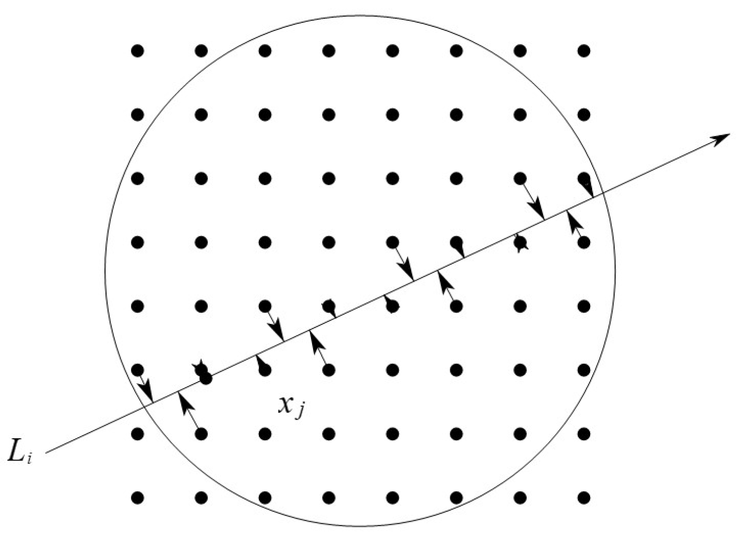
In the reconstructed points discretization model, the process of the beam attenuation can be described as the linear integral via the Beer theorem, as shown in Figure 1. The attenuation weight of the reconstruction point $x_j$ on the ray $L_i$ is denoted by $c_{ij}$, and the weight is determined by the distance $d_{ij}$ from the reconstruction point $x_j$ to the ray $L_i$, that is $c_{ij}=f\left(d_{ij}\right)$.

Let $x_j$ denote the attenuation coefficient of the j-th reconstructed point and $X={(x_1,x_2,\cdots x_N)}^T\in R^N$ denote the vector of the reconstructed points. The line integral of the projection process is discretized as:

$$b_i=\sum _{j=1}^N{c}_{ij}{x}_j$$

(7)

Here, $b_i$ stands for the projection value of the i-th ray, $c_{ij}$ the projection coefficient and $C={\left(c_{ij}\right)}_{M\times N}$ the projection coefficient matrix.

Since the M rays correspond to M linear equations, the linear system of equations can be obtained as follows.

$$b=CX+\delta +E$$

(8)

where $b={(b_1,b_2,\cdots b_N)}^T$ indicates the projection data, $C={\left(c_{ij}\right)}_{M\times N}$ the projection coefficient matrix, $\delta ={({\delta }_1,{\delta }_2,\cdots {\delta }_N)}^T$ the vector of errors from the discretization model and $E={(e_1,e_2,\cdots e_N)}^T$ the vector of errors from measurement and noise.

The projection coefficient matrix in the traditional discretization model consists of the intersection length between the square pixel and the ray. $C={\left(c_{ij}\right)}_{M\times N}$ is determined by the distance from the reconstructed point to the projection ray. The longer the distance is, the longer the projection coefficient is. Both the scanning model and the display model are considered in the reconstructed points discretization model. It overcomes the shortcoming that the intersection length changes with the angle, and it can describe the discretization expression of the line integral accurately.

As shown in Figure 2, the group $<T,*>$ is defined to describe the geometric symmetry of the conventional discretization model. The binary operation * is the successive transformation of the two transformations in $T=\{T_1,T_2,T_3,T_4,T_5,T_6,T_7,T_8\}$. $T_1$ and $T_2$ are the reflections on the x axis and y axis, respectively. $T_3$ and $T_4$ are the reflections on the $y=x$ axis and $y=-x$ axis. $T_5$, $T_6$ and $T_7$ are the rotations around the origin O counterclockwise by 90, 180 and 270 degrees. $T_8$ is the identity transformation.

The projection weights of all reconstructed points to the ray $L_i$ form one row vector of the matrix C. The eight symmetric projection rays possess the equivalent computation process of projection. We obtain the following theorem.

Theorem 1.

The algebraic system $<T,*>$ is a permutation group on S for the row vector $c_i=(c_{i1},c_{i2},\cdots c_{iN})$ of the matrix C, where $S=\{c_{i1},c_{i2},\cdots c_{iN}\}$.

$T_t\left(c_i\right)$ represents the transformation $T_t$ on the row vector $c_i$, where $t=1,2,\cdots 8$. $T_t\left(c_i\right)$ changes the order of the elements in $c_i$, i.e., $T_t\left(c_i\right)$ is the element replacement of the row vector $c_i$. The eight symmetric rays reveal the same projection weight sequence, but in different orders. If a row of the projection coefficient matrix is computed, the seven symmetric row vectors under the transformation group $<T,*>$ can be obtained by the permutation.

3. OSEM Algorithms Based on Symmetric Structure

Subset balancing is the key issue to affect the convergence rate and the imaging accuracy of OSEM algorithms. If the partitioning of subsets makes ${\sum }_{i\in I_k}{a}_{ij}$ equal for any point $x_j$ in each subset, the partitioning of subsets satisfies the balancing property of the subset. In this paper, the balancing property of subsets is approximatively satisfied in the two-dimensional parallel beam scanning computerized tomography, as a result of the rays in each subset being evenly distributed and each subset containing the same amount of information for image reconstruction.

The symmetry offers the strategies to select the subsets and optimize the iteration order. The symmetric rays are evenly distributed in the reconstructed region. The projection and the backprojection process the simplified computation structure due to the symmetry. Both the projection rays set and the reconstructed points set can be partitioned into the equivalence classes. The projection rays in the equivalent class possess the same projection computation process.

The projection data can be divided into subsets according to the projection angle. Then, the OSEM with the Symmetric Order (SO-OSEM) iterative algorithm can be established by utilizing the symmetry of angles to order the subsets. The OSEM with the Symmetric Subset (SS-OSEM) iterative algorithm is established by applying the symmetry of the projection rays in the subset to the compression calculation of the projection coefficient matrix.

3.1. SO-OSEM Iterative Algorithm

The set of projection rays’ angle indicators is denoted as $\varphi =\{1,2,\cdots ,N_{\varphi }\}$. $\varphi$ can be divided into ${\varphi }_1=\{1,2,\cdots ,N_{\varphi }/4\}$, ${\varphi }_2=\{N_{\varphi }/4+1,N_{\varphi }/4+2,\cdots ,N_{\varphi }/2\}$, ${\varphi }_3=\{N_{\varphi }/2+1,N_{\varphi }/4+2,\cdots ,3\times N_{\varphi }/4\}$ and ${\varphi }_4=\{3\times N_{\varphi }/4+1,3\times N_{\varphi }/4+2,\cdots ,N_{\varphi }\}$ according to the projection angle. ${\varphi }_1$, ${\varphi }_2$, ${\varphi }_3$ and ${\varphi }_4$ can be evenly divided into l blocks, respectively, and the q-th block of ${\varphi }_p$ is denoted as ${\varphi }_p^q$. Then ${\varphi }_l^q$, ${\varphi }_2^{l-q}$, ${\varphi }_3^q$ and ${\varphi }_4^{l-q}$ have the symmetry in angles.

The projection rays in block ${\varphi }_q^p$ form a subset in the SO-OSEM iterative algorithm. The order of the subset is ${\varphi }_1^1,{\varphi }_2^{(l-1)},{\varphi }_3^{(l-1)},{\varphi }_4^1,\cdots ,{\varphi }_1^{(l-1)},{\varphi }_2^1,{\varphi }_3^1,{\varphi }_4^{(l-1)}$. Here, $n=4\times l\times s (s=0,1,2,3,\cdots )$.

The SO-OSEM iterative algorithm is expressed as:

$$x_j^{(n+1)}=\frac{1}{{\sum }_{\phi \in {\varphi }_q^p}{\sum }_{i=1}^{N_d}{c}_{ij}^{\phi }}\sum _{\phi \in {\varphi }_q^p}\sum _{i=1}^{N_d}(\frac{c_{ij}^{\phi }{x}_j^{\left(n\right)}}{{\sum }_{j=1}^N{c}_{ij}^{\phi }{x}_j^{\left(n\right)}}{b}_i^{\phi })$$

(9)

The SO-OSEM iterative algorithm has two advantages. Firstly, the calculation of the projection coefficients is compressed by using the symmetric relationship of the rays in the same angle. Secondly, the iteration order of the subsets is improved by using the symmetric relationship of the angles between the subsets.

3.2. SS-OSEM Iterative Algorithm

Based on the partitioned blocks ${\varphi }_q^p$, the four symmetric blocks ${\varphi }_1^p$, ${\varphi }_2^p$, ${\varphi }_3^p$ and ${\varphi }_4^p$ can be merged into a block denoted as ${\varphi }^p$. The SS-OSEM algorithm takes the projection data belonging to the block ${\varphi }^p$ as a subset. The rays in the subset have a symmetrical relationship. The iterations of the subsets are performed in the order of ${\varphi }^p$.

The SS-OSEM iterative algorithm is expressed as:

$$x_j^{(n+1)}=\frac{1}{{\sum }_{\phi \in {\varphi }_q}{\sum }_{i=1}^{N_d}{c}_{ij}^{\phi }}\sum _{\phi \in {\varphi }_q}\sum _{i=1}^{N_d}(\frac{c_{ij}^{\phi }{x}_j^{\left(n\right)}}{{\sum }_{j=1}^N{c}_{ij}^{\phi }{x}_j^{\left(n\right)}}{b}_i^{\phi })$$

(10)

SS-OSEM iterative scheme has two advantages. Firstly, the symmetric relationship of the ray groups in the subset compresses the projection coefficient matrix calculation eight times. Secondly, the subset contains four symmetrical angles.

The SO-OSEM and SS-OSEM algorithms apply the symmetry between projection rays. The subsets are better balanced by using the symmetric relationship between rays to improve the order and the selection of the subsets. To improve the imaging precision, the order of the subsets is improved by the symmetry relationship between the rays, and the selection of the subsets approximately meets the balance property of the subsets. To accelerate the imaging speed, the calculation of the projection coefficient matrix is compressed simultaneously. Since the structure and properties of OS-SART and OSEM are similar, the OSEM iteration scheme with the symmetric structure properties can be transplanted into the OS-SART iterative scheme.

The iterative process of SO-OSEM and SS-OSEM (Algorithm 1) is as follows.

Algorithm 1 The iterative process of Symmetric Order (SO)-OSEM and Symmetric Subset (SS)-OSEM algorithms.
1: procedure Iterative(Projection data b)	▹ Image reconstruction from projection data b
2:  $n\leftarrow 0$;
3:  while $△X^{\left(n\right)}>\epsilon$ and $n<N$ do	▹ $△X^{\left(n\right)}\le \epsilon$ and $n\ge N$ are the stop criteria
4:   $k=\left(n\mathrm{mod}K\right)+1$;
5:   $n\leftarrow n+1$;
6:   if method = SO-OSEM then
7:      $X^{\left(n\right)}\leftarrow \mathbf{\text{SO-OSEM}}(X^{(n-1)},b_k)$;
8:   else
9:      $X^{\left(n\right)}\leftarrow \mathbf{\text{SS-OSEM}}(X^{(n-1)},b_k)$;
10:   end if
11:   $△X^{\left(n\right)}=X^{\left(n\right)}-X^{(n-1)}$;
12:  end while
13:  $X^{*}=X^{\left(n\right)}$
14:  return $X^{*}$	▹ The reconstruction result is $X^{*}$
15: end procedure

4. Experimental Results

In the experiments, the results of reconstruction applying SO-OSEM and SS-OSEM iterative algorithms are shown and analyzed. We validate the SO-OSEM and SS-OSEM iterative algorithms via both the simulated data and the real data. The simulated image emphasized the reconstruction accuracy of the fine texture. The real data applied ceramic blades of a certain type of engine, and the reconstructed image emphasized the reconstruction accuracy of small cracks. We compared the results of the proposed algorithms with the reconstruction results of the ART, EM, BIP and SAP algorithms. The error analysis was performed by the Root-Mean-Squared Error (RMSE), and also, the imaging results were analyzed and compared by using the profile. The number of subsets in SO-OSEM and SS-OSEM iterative algorithms is 36. Figure 3 shows the simulated original image. The simulation results are shown in Figure 4 and Figure 5. Figure 6 shows the real projection data. The real data results are shown in Figure 7 and Figure 8.

Table 1. Reconstruction analysis of the simulated data.

Algorithm	Iterations	RMSE	Time (s)
EM	40	0.360006	118.6756051
ART	5	0.400026	40.2356841
BIP	3	0.488761	27.641001
SAP	3	0.375179	20.2152612
OSEM-SO	3	0.225890	10.0556901
OSEM-SS	3	0.207040	10.065243

shows the reconstruction error of the simulated data. The experiments were carried out via Microsoft Visual Studio 2015 on a PC (8.0 Gigabyte memory, 2.93 GHz CPU).

The RMSE is defined as:

$$d=\sqrt{\frac{{\sum }_{i=1}^N{\sum }_{j=1}^N{(t_{ij}-r_{ij})}^2}{{\sum }_{i=1}^N{\sum }_{j=1}^N{(t_{ij}-\overline{t})}^2}}$$

(11)

where $t_{ij}$ and $r_{ij}$ represent the pixel values of the i-th row and the j-th column of the original image and the reconstructed image, respectively. $\overline{t}$ represents the mean value of the original image pixel values.

Experimental results show that the SO-OSEM and SS-OSEM algorithms have a significant improvement in accuracy and a stronger ability to recover details compared to the EM, ART, BIP and SAP algorithms. The reconstruction error of approximately 0.2 can be achieved with only three iterations with a faster convergence rate than the EM algorithm. At the same time, the calculation speed of the reconstruction is also greatly improved by compressing the calculation of the projection coefficient matrix.

It can be seen from the profiles of the simulated data and the real data that the spatial resolution and density resolution of the reconstruction results of the algorithm are improved. The profiles of the·image reconstructed by the algorithm proposed in this paper are relatively flat. The detail features can be better reconstructed to reveal the fine crack characteristics of the ceramic blades. Both simulation results (Figure 4 and Figure 5) and real data results (Figure 7) show that the SO-OSEM and SS-OSEM iterative algorithms make good use of the symmetric structure and optimize the subset balance and the iteration order to improve the image quality and simplify the compression of the projection coefficient matrix calculation.

5. Summary

In this paper, we applied the symmetric relationship of projection rays to the construction of OSEM algorithms and to improve the order and selection of subsets, which can approximately meet the balancing of subsets and improve the imaging accuracy. In addition, the calculation of the projection coefficient matrix can be compressed, which improves the imaging speed. Based on the reconstruction discretization model, its related symmetric properties can be applied to solve the problem of acceleration, incomplete data, subset selection, subset order and noise suppression. Under the transformation group of symmetry, the positional relationship of the projection rays and the pixels are invariant. In the process of iterative correction, the symmetry structure property can be applied to optimize and improve the reconstruction algorithm.

The discretization model is fundamental in image reconstruction to solve the reconstruction problem from continuous space to discrete space. The study on the design of the image reconstruction discretization model and its related geometric properties is of great significance for solving the practical problems existing in the medical and industrial CT. The symmetry structure property in geometry is independent of the object reconstructed and does not depend on the projection data. It is the basic property of the reconstruction model and the basic internal relationship between the discrete form of the image and the discrete projection data. The symmetry structure properties can be extended to fan beam scanning modes and three-dimensional imaging models. The ideas and related methods of the discretization model can also be applied to other inverse problems.