Eventually DSDD Matrices and Eigenvalue Localization

Abstract

Firstly, the relationships among strictly diagonally dominant ($SDD$) matrices, doubly strictly diagonally dominant ($DSDD$) matrices, eventually $SDD$ matrices and eventually $DSDD$ matrices are considered. Secondly, by excluding some proper subsets of an existing eigenvalue inclusion set for matrices, which do not contain any eigenvalues of matrices, a tighter eigenvalue inclusion set of matrices is derived. As its application, a sufficient condition of determining non-singularity of matrices is obtained. Finally, the infinity norm estimation of the inverse of eventually $DSDD$ matrices is derived.

1. Introduction

Let n be a positive integer, $n\ge 2$, $\mathcal{J}=\{1,2,\cdots ,n\}$, N be the set of all positive integers, $\mathbb{C}$ be the set of all complex numbers, ${\mathbb{C}}^{n\times n}$ be the set of all $n\times n$ complex matrices and I be the identity matrix. Let $A=[a_{ij}]\in {\mathbb{C}}^{n\times n}$ and $\sigma (A)$ be the set of all eigenvalues of A. For $i,j\in \mathcal{J},j\ne i$, denote $r_i(A):={\displaystyle \sum _{t\in \mathcal{J},t\ne i}}|a_{it}|$ and $r_i^j(A):=r_i(A)-|a_{ij}|$. A matrix A is called a strictly diagonally dominant ($SDD$) matrix if, for each $i\in \mathcal{J}$,

$$|a_{ii}|>r_i(A).$$

In addition, A is doubly strictly diagonally dominant ($DSDD$) if, for any $i,j\in \mathcal{J},i\ne j$,

$$|a_{ii}||a_{jj}|>r_i(A)r_j(A).$$

Locating eigenvalue and bounding infinity norm of the inverse for nonsingular matrices are two major problems in applied linear algebra [1,2,3,4,5,6,7]. The first problem is to find a set in the complex plane to include all eigenvalues of matrices, as if the obtained set is on the right-hand side of the complex plane. Then, one can conclude the positive definiteness of the corresponding matrix. Moreover, the “eigenvalue localization” is very important for the convergence speed of algorithms on which web searching engines are based. For the case of PageRank, see [4] and references therein. Another problem is to bound the infinity norm for the inverse of nonsingular matrices, as it can be used to estimate the condition number for the linear systems of equations [5], as well as linear complementarity problems [6]. In general, it is not easy to discuss these two problems for an arbitrary given nonsingular matrix. One traditional way for solving the two problems is to locate all eigenvalues or to bound the infinity norm for some subclasses of nonsingular matrices.

In 2015, Cvetković [7] et al. extended the class of $SDD$ matrices to the class of eventually $SDD$ ($SD{D}_{\exists }$) matrices, and proved that $SD{D}_{\exists }$ matrices are nonsingular.

Definition 1

([7], Definition 1). Let $A=sI-B$, where $s\in \mathbb{C}$. A is called an $SD{D}_{\exists }$ matrix if $s^{k}I-B^k$ is $SDD$ for a positive integer k.

To bound the infinity norm for the inverse of $SD{D}_{\exists }$ matrices, Cvetković et al. [7] gave the following results.

Theorem 1

([7], Theorem 2). Let $A\in SD{D}_{\exists }$. Then, for two certain numbers s and k,

$$\begin{array}{c}\hfill ||A^{-1}{||}_{\infty }\le {\Psi }_k^s(A)=\frac{||s^{k-1}I+s^{k-2}B+\cdots +s{B}^{k-2}+B^{k-1}{||}_{\infty }}{\underset{i\in \mathcal{J}}{\min }\{|s^k-{(B^k)}_{ii}|-r_i(B^k)\}}.\end{array}$$

It is worth noting in Theorem 1 that, from Examples 3 and 4 in [7] and the structure of ${\Psi }_k^s(A)$, which includes two parameters s and k, one can conclude that, if there exists two groups of different numbers s and k, both such that A is an $SD{D}_{\exists }$ matrix, then the different selection of s and k will affect the infinity norm bounds for the inverse of A.

According to the non-singularity of $SD{D}_{\exists }$ matrices, Liu et al. [8] obtained the following eigenvalue inclusion set of matrices, which corrects Theorem 1 of [7].

Theorem 2

([8], Theorem 2). Let $A=sI-B\in {\mathbb{C}}^{n\times n}$. For any given positive integer k,

$$\sigma (A)\subseteq {\Gamma }_k^s(A)=\bigcup _{i\in \mathcal{J}}\left\{{z\in \mathbb{C}:|(s-z)}^k-{(B^k)}_{ii}|\le r_i(B^k)\right\}.$$

In 2016, Liu [9] introduced the class of eventually $DSDD$ ($DSD{D}_{\exists }$) matrices, and located all its eigenvalues.

Definition 2

([9], Definition 3.2.1). Let $A=sI-B$, where $s\in \mathbb{C}$. A is called an $DSD{D}_{\exists }$ matrix if $s^{k}I-B^k$ is $DSDD$ for a positive integer k.

Remark 1.

From Definition 2, a meaningful discussion is concerned:

$$Is s^{K}I-B^K DSDD if s^{k}I-B^k with k<K has this property?$$

Unfortunately, the answer is negative. Let

$$B=\left[\begin{array}{ccc}1& 0& 1\\ 1& 4& 1\\ 1& 1& 4\end{array}\right],s=0,andK=2.$$

It is easy to validate that, if $k=1$, then $s^{k}I-B^k=-B$ is $DSDD$, and that $s^{K}I-B^K=-B^2$ is not $DSDD$.

Theorem 3

([9], Theorem 3.3.1). Let $A=sI-B\in {\mathbb{C}}^{n\times n}$. For any given positive integer k,

$$\sigma (A)\subseteq {\Omega }_k^s(A)=\bigcup _{i,j\in \mathcal{J},i\ne j}{\Omega }_{i,j}^s(B^k),$$

and

$$\begin{array}{c}\hfill {\Omega }_{i,j}^s(B^k)=\left\{{z\in \mathbb{C}:|(s-z)}^k-{(B^k)}_{ii}||{(s-z)}^k-{(B^k)}_{jj}|\le r_i(B^k)r_j(B^k)\right\}.\end{array}$$

Note here that, when $k=1$, the sets ${\Omega }_{i,j}^s(B^k)$ in Theorem 3 are ovals, while the sets ${\Omega }_{i,j}^s(B^k)$ with $k\ge 2$ are lemniscates; see [10] (pp. 35–52), for details.

As everyone knows that $SDD$ matrices are $DSDD$ matrices and $DSDD$ matrices are nonsingular, hence,

$$\begin{array}{c}\hfill \{SDD\}\subseteq \{DSDD\}\subseteq \{Nonsingular\}.\end{array}$$

(1)

By Label (1), and Definitions 1 and 2, the following two relations hold clearly:

$$\begin{array}{c}\hfill \{SDD\}\subseteq \{SD{D}_{\exists }\}\subseteq \{DSD{D}_{\exists }\}\subseteq \{Nonsingular\}\end{array}$$

and

$$\begin{array}{c}\hfill \{SDD\}\subseteq \{DSDD\}\subseteq \{DSD{D}_{\exists }\}\subseteq \{Nonsingular\}.\end{array}$$

Besides $SDD$ matrices, $DSDD$ matrices, $SD{D}_{\exists }$ matrices and $DSD{D}_{\exists }$ matrices, there are many other subclasses of nonsingular matrices; see [11] for details.

The outline of the rest of this paper is as follows. In Section 2, by some existing criteria for non-singularity of matrices, a new eigenvalue localization set of matrices is derived. That is, a tighter eigenvalue localization set is obtained by excluding some proper subsets from ${\Omega }_{i,j}^s(B^k)$ in Theorem 3, which is proved to not include any eigenvalues of matrices. In Section 3, the infinity norm for the inverse of $DSD{D}_{\exists }$ matrices is given. Finally, some concluding remarks are given in Section 4 to summarize this paper.

2. Eigenvalue Localization of Matrices

Firstly, a lemma in [12] is listed, which is very useful for deriving a new eigenvalue inclusion set.

Lemma 1

([12, Corollary 1]). Let $A=[a_{ij}]\in {\mathbb{C}}^{n\times n}$. If for each $i,j\in \mathcal{J}$, $j\ne i$, either

$$|a_{ii}||a_{jj}|>r_i(A)r_j(A)$$

or

$$(|a_{ii}|+r_i^t(A))|a_{tt}|<|a_{it}|(|a_{ti}|-r_t^i(A))$$

for some $t\ne i$ and $t\in \mathcal{J}$, then A is nonsingular.

Lemma 2.

Let $A=sI-B\in {\mathbb{C}}^{n\times n}$. For any given positive integer k,

$$\sigma (A)\subseteq {\Delta }_k^s(A)=\bigcup _{i,j\in \mathcal{J},j\ne i}\left[{\Omega }_{i,j}^s(B^k)\backslash {\Delta }_i^s(B^k)\right],$$

where

$$\begin{array}{c}\hfill {\Delta }_i^s(B^k)=\bigcup _{t\in \mathcal{J},t\ne i}{\Delta }_{i,t}^s(B^k),\end{array}$$

and

$$\begin{array}{c}\hfill {\Delta }_{i,t}^s(B^k)=\left\{z\in \mathbb{C}:\left({|(s-z)}^k-{(B^k)}_{ii}|+r_i^t(B^k)\right){|(s-z)}^k-{(B^k)}_{tt}|<|{(B^k)}_{it}|\left(|{(B^k)}_{ti}|-r_t^i(B^k)\right)\right\}.\end{array}$$

Proof. 

Let $\lambda \in \sigma (A)$. Given k, suppose that $\lambda \notin {\Delta }_k^s(A)$, i.e., for any $i,j\in \mathcal{J},i\ne j$, $\lambda \notin \left[{\Omega }_{i,j}^s(B^k)\backslash {\Delta }_i^s(B^k)\right]$, which is equivalent to that $\lambda \notin {\Omega }_{ij}^s(B^k)$ or $\lambda \in {\Delta }_i^s(B^k)={\displaystyle \bigcup _{t\in \mathcal{J},t\ne i}}{\Delta }_{i,t}^s(B^k)$, then

$$\begin{array}{c}\hfill {|(s-\lambda )}^k-{(B^k)}_{ii}||{(s-\lambda )}^k-{(B^k)}_{jj}|>r_i(B^k)r_j(B^k),\end{array}$$

or for some $t\in \mathcal{J},t\ne i$,

$$\begin{array}{c}\hfill \left({|(s-\lambda )}^k-{\left(B^k\right)}_{ii}|+r_i^t\left(B^k\right)\right){|(s-\lambda )}^k-{\left(B^k\right)}_{tt}|<|{\left(B^k\right)}_{it}|(|{\left(B^k\right)}_{ti}|-r_t^i\left(B^k\right)).\end{array}$$

Then, by Lemma 1, we have ${(s-\lambda )}^{k}I-B^k$ is nonsingular, i.e., ${(s-\lambda )}^k$ is not an eigenvalue of $B^k$. On the other hand, because $\lambda \in \sigma \left(A\right)$, there is a vector x, $x\ne 0$, such that $Bx=(s-\lambda )x$. Furthermore, we have $B^{k}x={(s-\lambda )}^{k}x$, which implies that ${(s-\lambda )}^k$ is an eigenvalue of $B^k$. This is a contradiction. Hence, $\lambda \in {\Delta }_k^s\left(A\right)$. The conclusion holds. ☐

By the arbitrariness of $s\in \mathbb{C}$ and $k\in N$ in Lemma 2, the following eigenvalue localization theorem is obtained easily.

Theorem 4.

Let $A=sI-B\in {\mathbb{C}}^{n\times n}$. Then,

$$\sigma \left(A\right)\subseteq \Delta \left(A\right)=\bigcap _{s\in \mathbb{C}}\bigcap _{k\in N}{\Delta }_k^s\left(A\right).$$

For all $i,j\in \mathcal{J},i\ne j$, the relationship

$${\Omega }_{i,j}^s\left(B^k\right)\backslash {\Delta }_i^s\left(B^k\right)={\Omega }_{i,j}^s\left(B^k\right)\cap \overline{{\Delta }_i^s\left(B^k\right)}\subseteq {\Omega }_{i,j}^s\left(B^k\right)$$

holds, hence the following comparison theorem for Theorem 3, Lemma 2 and Theorem 4 is given easily.

Theorem 5.

Let $A=sI-B\in {\mathbb{C}}^{n\times n}$. Given an arbitrary positive integer k, then

$$\Delta \left(A\right)\subseteq {\Delta }_k^s\left(A\right)\subseteq {\Omega }_k^s\left(A\right)\subseteq {\Gamma }_k^s\left(A\right).$$

Note here that, from the proof of Lemma 2, it can be seen that ${\Delta }_{i,t}^s\left(B^k\right)$ does not contain any eigenvalues of A, and that ${\Delta }_k^s\left(A\right)$ is derived by excluding some proper subsets ${\Delta }_{i,t}^s\left(B^k\right)$ from ${\Omega }_{i,j}^s\left(B^k\right)$. Hence, ${\Delta }_{i,t}^s\left(B^k\right)$ is called an exclusion set of ${\Delta }_k^s\left(A\right)$. By Theorem 5, one can exclude some regions that do not include any eigenvalues of matrices to locate them more precisely.

Taking $s=0,k=1$ in Theorem 4, the following result, which is also Theorem 4 in [12], is deduced immediately.

Corollary 1.

Let $A=\left[a_{ij}\right]\in {\mathbb{C}}^{n\times n}$. Then,

$$\sigma \left(A\right)\subseteq \overline{\Delta }\left(A\right)=\bigcup _{i,j\in \mathcal{J},j\ne i}\left[{\Omega }_{i,j}\left(A\right)\backslash {\Delta }_i\left(A\right)\right],$$

where

$$\begin{array}{c}\hfill {\Delta }_i\left(A\right)=\bigcup _{t\in \mathcal{J},t\ne i}{\Delta }_{i,t}\left(A\right),\end{array}$$

and

$$\begin{array}{c}\hfill {\Omega }_{i,j}\left(A\right)=\left\{z\in \mathbb{C}:|z-a_{ii}||z-a_{jj}|\le r_i\left(A\right)r_j\left(A\right)\right\},\end{array}$$

$$\begin{array}{c}\hfill {\Delta }_{i,t}\left(A\right)=\left\{z\in \mathbb{C}:\left(|z-a_{ii}|+r_i^t\left(A\right)\right)|z-a_{tt}|<|a_{it}|(|a_{ti}|-r_t^i\left(A\right))\right\}.\end{array}$$

Next, based on Lemma 2 and the fact that $\det \left(A\right)=0$ if and only if $0\in \sigma \left(A\right)$ for a matrix A, the following condition such that $\det \left(A\right)\ne 0$ is given easily.

Corollary 2.

Let $A=sI-B\in {\mathbb{C}}^{n\times n}$. If there is a positive integer k such that for any $i,j\in \mathcal{J},i\ne j$, either

$$\begin{array}{c}\hfill |s^k-{\left(B^k\right)}_{ii}||s^k-{\left(B^k\right)}_{jj}|>r_i\left(B^k\right)r_j\left(B^k\right),\end{array}$$

or for some $t\ne i$ and $t\in \mathcal{J}$,

$$\begin{array}{c}\hfill \left(|s^k-{\left(B^k\right)}_{ii}|+r_i^t\left(B^k\right)\right)|s^k-{\left(B^k\right)}_{tt}|<|{\left(B^k\right)}_{it}|\left(|{\left(B^k\right)}_{ti}|-r_t^i\left(B^k\right)\right),\end{array}$$

then A is nonsingular.

Note here that, if taking $s=0$ and $k=1$, then Corollary 2 is reduced to Lemma 1. That is to say, Corollary 2 is a generalization of Lemma 1.

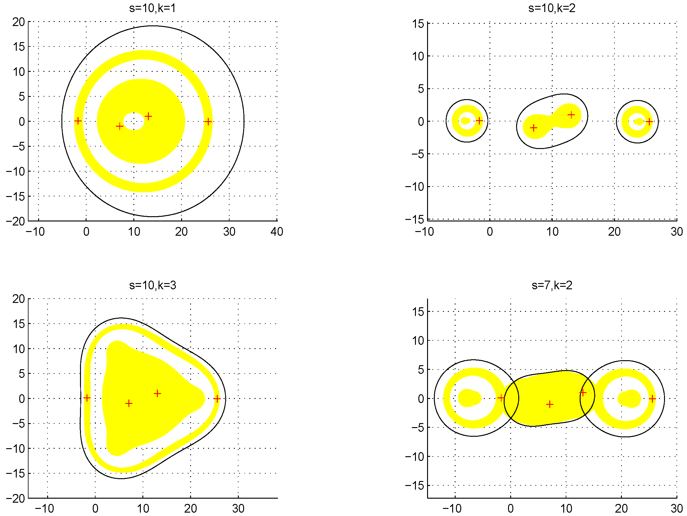
Finally, an example is given to validate Theorem 5, and show that the different selection of s and k will affect the eigenvalue location and the determination of non-singularity of $A=sI-B$.

Example 1.

Consider the matrix provided in [12]:

$$A=\left[\begin{array}{cccc}14& 0.01\mathit{i}& 0& 18-2\mathit{i}\\ 0& 9& 4+\mathit{i}& 0\\ 0.01+\mathit{i}& 2+\mathit{i}& 11& 0\\ 10+\mathit{i}& 0& 0.1+\mathit{i}& 10\end{array}\right].$$

By computation, the spectrum of A is

$$\sigma \left(A\right)=\{25.5919-0.0647\mathit{i},-1.6930+0.0821\mathit{i},13.0618+0.9825\mathit{i},7.0393-0.9999\mathit{i}\}.$$

The eigenvalue inclusion set ${\Gamma }_k^s\left(A\right)$, ${\Omega }_k^s\left(A\right)$ and ${\Delta }_k^s\left(A\right)$ with different s and k, and all eigenvalues are drawn in Figure 1, where ${\Gamma }_k^s\left(A\right)$, ${\Omega }_k^s\left(A\right)$ and ${\Delta }_k^s\left(A\right)$, respectively, are showed by black boundary, yellow zone and its interior, and yellow zone. All eigenvalues are plotted by ‘+’.

From Figure 1, it can be seen that:

(1)

Whether $s=10,k=1,2,3$ or $s=7,k=2$, it can be seen that

$$\sigma \left(A\right)\subseteq {\Delta }_k^s\left(A\right)\subseteq {\Omega }_k^s\left(A\right)\subset {\Gamma }_k^s\left(A\right)$$

obtained by Theorem 1 for the same k and s.

(2)

When $s=10$, if taking $k=1$, $k=2$ and $k=3$, then differences of the three eigenvalue inclusion sets ${\Delta }_1^{10}\left(A\right)$, ${\Delta }_2^{10}\left(A\right)$, ${\Delta }_3^{10}\left(A\right)$ are clear. This implies that, if s is the same, but k is different, then these eigenvalue inclusion sets ${\Delta }_k^s\left(A\right)$ are different in general.

(3)

When $k=2$, if taking $s=7$ and $s=10$, then the two eigenvalue inclusion sets ${\Delta }_2^2\left(A\right)$ and ${\Delta }_2^{10}\left(A\right)$ are also different, which implies that, if k is the same, but s is different, then these eigenvalue inclusion sets ${\Delta }_k^s\left(A\right)$ are also different in general.

(4)

When $s=7$ and $k=2$, we can see that $0\in {\Delta }_2^7\left(A\right)$. When $s=10$ and $k=1,2,3$, we can see that $0\notin {\Delta }_1^{10}\left(A\right)$, $0\notin {\Delta }_2^{10}\left(A\right)$ and $0\notin {\Delta }_3^{10}\left(A\right)$. That is to say, we cannot determine the non-singularity of A when $s=7$ and $k=2$, but we can do it when $s=10$ and $k=1,2,3$, respectively. When k is the same one, the upper bounds ${\Theta }_k^5\left(A\right)$ and ${\Psi }_k^5\left(A\right)$, respectively, are less than or equal to the upper bounds ${\Theta }_k^4\left(A\right)$ and ${\Theta }_k^{10}\left(A\right)$, and ${\Psi }_k^4\left(A\right)$ and ${\Psi }_k^{10}\left(A\right)$. In addition, if taking $s=5$ and $k=8$, the upper bound ${\Theta }_8^5\left(A\right)={\Psi }_8^5\left(A\right)=0.4657$, which reaches the true value of $||A^{-1}{||}_{\infty }$.

Then, an interesting problem is considered naturally: how to choose s and k to minimize the eigenvalue inclusion set ${\Delta }_k^s\left(A\right)$ and determine the non-singularity of $A=sI-B$? Hence, it is essential to study this question in the future.

3. Infinity Norm Bounds for the Inverse of ${\mathit{DSDD}}_{\mathbf{\exists }}$ Matrices

Firstly, a lemma is listed, which is used to obtain the infinity norm bounds for the inverse of $DSD{D}_{\exists }$ matrices.

Lemma 3

([13]). If $A\in DSDD$, then

$$\begin{array}{c}\hfill ||A^{-1}{||}_{\infty }\le \underset{i,j\in \mathcal{J},i\ne j}{\max }\frac{|a_{ii}|+r_j\left(A\right)}{|a_{ii}||a_{jj}|-r_i\left(A\right)r_j\left(A\right)}.\end{array}$$

Theorem 6.

Let $A\in DSD{D}_{\exists }$. Then, for two certain numbers s and k,

$$\begin{array}{c}\hfill ||A^{-1}{||}_{\infty }\le {\Theta }_k^s\left(A\right)=\underset{i,j\in \mathcal{J},i\ne j}{\max }\frac{\left(|s^k-{\left(B^k\right)}_{ii}|+r_j\left(B^k\right)\right)||s^{k-1}I+s^{k-2}B+\cdots +s{B}^{k-2}+B^{k-1}{||}_{\infty }}{|s^k-{\left(B^k\right)}_{ii}||s^k-{\left(B^k\right)}_{jj}|-r_i\left(B^k\right)r_j\left(B^k\right)}.\end{array}$$

(2)

Proof. 

Since $A\in DSD{D}_{\exists }$, there exists $k\in N$ such that $s^{k}I-B^k\in DSDD$. Obviously, A and $s^{k}I-B^k$ are both nonsingular. By

$$s^{k}I-B^k=(sI-B)(s^{k-1}I+s^{k-2}B+\cdots +s{B}^{k-2}+B^{k-1}),$$

we have

$${(sI-B)}^{-1}={(s^{k}I-B^k)}^{-1}(s^{k-1}I+s^{k-2}B+\cdots +s{B}^{k-2}+B^{k-1}).$$

Then,

$$||A^{-1}{||}_{\infty }\le ||{(s^{k}I-B^k)}^{-1}{||}_{\infty }||s^{k-1}I+s^{k-2}B+\cdots +s{B}^{k-2}+B^{k-1}{||}_{\infty }.$$

Since $s^{k}I-B^k\in DSDD$, by Lemma 3, we have

$$||{(s^{k}I-B^k)}^{-1}{||}_{\infty }\le \underset{i,j\in \mathcal{J},i\ne j}{\max }\frac{|s^k-{\left(B^k\right)}_{ii}|+r_j\left(B^k\right)}{|s^k-{\left(B^k\right)}_{ii}||s^k-{\left(B^k\right)}_{jj}|-r_i\left(B^k\right)r_j\left(B^k\right)}.$$

This implies that Label (2) holds. The proof is completed. ☐

Lemma 4.

If A is $SDD$, then

$$\underset{i,j\in \mathcal{J},i\ne j}{\max }\frac{|a_{ii}|+r_j\left(A\right)}{|a_{ii}||a_{jj}|-r_i\left(A\right)r_j\left(A\right)}\le \frac{1}{\underset{i\in \mathcal{J}}{\min }\{|a_{ii}|-r_i\left(A\right)\}}.$$

(3)

Proof. 

Since A is $SDD$, i.e., $|a_{ii}|>r_i\left(A\right),i\in \mathcal{J},$ hence $|a_{ii}||a_{jj}|>r_i\left(A\right)r_j\left(A\right),i,j\in \mathcal{J},i\ne j$. In order to obtain Label (3), it is sufficient to show that for all $i,j\in \mathcal{J},i\ne j$, the following inequality holds:

$$\begin{array}{c}\hfill \frac{|a_{ii}|+r_j\left(A\right)}{|a_{ii}||a_{jj}|-r_i\left(A\right)r_j\left(A\right)}\le \frac{1}{\min \left\{|a_{ii}|-r_i\left(A\right),|a_{jj}|-r_j\left(A\right)\right\}}.\end{array}$$

Indeed, if

$$|a_{jj}|-r_j\left(A\right)\le |a_{ii}|-r_i\left(A\right),$$

then multiplying this inequality with $r_j\left(A\right)$ gives

$$|a_{jj}|r_j\left(A\right)-{\left(r_j\left(A\right)\right)}^2\le |a_{ii}|r_j\left(A\right)-r_i\left(A\right)r_j\left(A\right),$$

i.e.,

$$|a_{ii}||a_{jj}|-|a_{ii}|r_j\left(A\right)+|a_{jj}|r_j\left(A\right)-{\left(r_j\left(A\right)\right)}^2\le |a_{ii}||a_{jj}|-r_i\left(A\right)r_j\left(A\right).$$

This can be rewritten as

$$\left(|a_{ii}|+r_j\left(A\right)\right)\left(|a_{jj}|-r_j\left(A\right)\right)\le |a_{ii}||a_{jj}|-r_i\left(A\right)r_j\left(A\right),$$

i.e.,

$$\begin{array}{c}\hfill \frac{|a_{ii}|+r_j\left(A\right)}{|a_{ii}||a_{jj}|-r_i\left(A\right)r_j\left(A\right)}\le \frac{1}{|a_{jj}|-r_j\left(A\right)}=\frac{1}{\min \left\{|a_{ii}|-r_i\left(A\right),|a_{jj}|-r_j\left(A\right)\right\}}.\end{array}$$

On the contrary, if

$$|a_{ii}|-r_i\left(A\right)\le |a_{jj}|-r_j\left(A\right),$$

multiplying this inequality with $|a_{ii}|$, we get

$$|a_{ii}{|}^2-r_i\left(A\right)|a_{ii}|\le |a_{ii}||a_{jj}|-|a_{ii}|r_j\left(A\right),$$

i.e.,

$$|a_{ii}{|}^2-|a_{ii}|r_i\left(A\right)+|a_{ii}|r_j\left(A\right)-r_i\left(A\right)r_j\left(A\right)\le |a_{ii}||a_{jj}|-r_i\left(A\right)r_j\left(A\right),$$

which can be rewritten as

$$\left(|a_{ii}|+r_j\left(A\right)\right)\left(|a_{ii}|-r_i\left(A\right)\right)\le |a_{ii}||a_{jj}|-r_i\left(A\right)r_j\left(A\right),$$

i.e.,

$$\begin{array}{c}\hfill \frac{|a_{ii}|+r_j\left(A\right)}{|a_{ii}||a_{jj}|-r_i\left(A\right)r_j\left(A\right)}\le \frac{1}{|a_{ii}|-r_i\left(A\right)}=\frac{1}{\min \left\{|a_{ii}|-r_i\left(A\right),|a_{jj}|-r_j\left(A\right)\right\}}.\end{array}$$

The proof is completed. ☐

Next, a comparison for the bounds in Theorems 1 and 6 is given.

Theorem 7.

If $A\in SD{D}_{\exists }$, then, for two certain numbers s and k,

$$\begin{array}{c}\hfill {\Theta }_k^s\left(A\right)\le {\Psi }_k^s\left(A\right).\end{array}$$

(4)

Proof. 

Since $A\in SD{D}_{\exists }$, i.e., for some $s\in \mathbb{C}$ and some $k\in N$, $s^{k}I-B^k$ is $SDD$, then by Lemma 4, we have

$$\begin{array}{c}\hfill \underset{i,j\in \mathcal{J},i\ne j}{\max }\frac{\left(|s^k-{\left(B^k\right)}_{ii}|+r_j\left(B^k\right)\right)}{|s^k-{\left(B^k\right)}_{ii}||s^k-{\left(B^k\right)}_{jj}|-r_i\left(B^k\right)r_j\left(B^k\right)}\le \frac{1}{\min \left\{|s^k-{\left(B^k\right)}_{ii}|-r_i\left(B^k\right),|s^k-{\left(B^k\right)}_{jj}|-r_j\left(B^k\right)\right\}}.\end{array}$$

Furthermore, by $||s^{k-1}I+s^{k-2}B+\cdots +s{B}^{k-2}+B^{k-1}{||}_{\infty }\ge 0$, Label (4) holds clearly. ☐

Finally, an example is given to validate Theorem 7, and show that the different selection of s and k will affect the infinity norm bounds for the inverse of $A=sI-B$.

Example 2.

Consider the matrix provided in [7]:

$$A=\left[\begin{array}{ccccc}\hfill 3.9& \hfill -1& \hfill -1& \hfill -1& \hfill 1\\ \hfill 1& \hfill 5.9& \hfill 1& \hfill 1& \hfill -1\\ \hfill -1& \hfill -1& \hfill 3.9& \hfill -1& \hfill 1\\ \hfill 1& \hfill 1& \hfill 1& \hfill 5.9& \hfill -1\\ \hfill -1& \hfill -1& \hfill -1& \hfill -1& \hfill 3.9\end{array}\right].$$

By computations, $||A^{-1}{||}_{\infty }=0.4657.$ Taking $s=4$, 5 and 10 for $k=2,\cdots ,10$, respectively, we can validate that $s^{k}I-B^k$ are all $SDD$ matrices. Obviously, they are all $DSDD$ matrices too. Thus, we can use Theorems 1 and 6 to estimate $||A^{-1}{||}_{\infty }$. The numerical results are listed in

Table 1. Comparisons of ${\Psi }_k^s\left(A\right)$ and ${\Theta }_k^s\left(A\right)$ with different s and k.

	${\mathbf{\Psi }}_{\mathit{k}}^{\mathbf{4}}\mathbf{\left(}\mathit{A}\mathbf{\right)}$	${\mathbf{\Theta }}_{\mathit{k}}^{\mathbf{4}}\mathbf{\left(}\mathit{A}\mathbf{\right)}$	${\mathbf{\Psi }}_{\mathit{k}}^{\mathbf{5}}\mathbf{\left(}\mathit{A}\mathbf{\right)}$	${\mathbf{\Theta }}_{\mathit{k}}^{\mathbf{5}}\mathbf{\left(}\mathit{A}\mathbf{\right)}$	${\mathbf{\Psi }}_{\mathit{k}}^{\mathbf{10}}\mathbf{\left(}\mathit{A}\mathbf{\right)}$	${\mathbf{\Theta }}_{\mathit{k}}^{\mathbf{10}}\mathbf{\left(}\mathit{A}\mathbf{\right)}$
$k=2$	2.5392	2.5392	0.5319	0.5245	1.1173	0.9454
$k=3$	0.6152	0.6152	0.4775	0.4774	0.7152	0.6472
$k=4$	0.5118	0.5118	0.4682	0.4682	0.5939	0.5608
$k=5$	0.4764	0.4764	0.4663	0.4663	0.5388	0.5224
$k=6$	0.4690	0.4690	0.4658	0.4658	0.5094	0.5014
$k=7$	0.4665	0.4665	0.4658	0.4658	0.4925	0.4887
$k=8$	0.4659	0.4659	0.4657	0.4657	0.4823	0.4806
$k=9$	0.4658	0.4658	0.4657	0.4657	0.4760	0.4754
$k=10$	0.4657	0.4657	0.4657	0.4657	0.4721	0.4719

.

Numerical results in Table 1 show that:

(1)

The upper bound ${\Theta }_k^s\left(A\right)$ obtained by Theorem 6 is less than or equal to the bound ${\Psi }_k^s\left(A\right)$ obtained by Theorem 1 for the same k and s.

(2)

When s is the same, the upper bounds ${\Theta }_k^s\left(A\right)$ and ${\Psi }_k^s\left(A\right)$ do not increase with the increase of k. When k is the same one, the upper bounds ${\Theta }_k^5\left(A\right)$ and ${\Psi }_k^5\left(A\right)$, respectively, are less than or equal to the upper bounds ${\Theta }_k^4\left(A\right)$ and ${\Theta }_k^{10}\left(A\right)$, and ${\Psi }_k^4\left(A\right)$ and ${\Psi }_k^{10}\left(A\right)$. In addition, if taking $s=5$ and $k=8$, the upper bound ${\Theta }_8^5\left(A\right)={\Psi }_8^5\left(A\right)=0.4657$, which reaches the true value of $||A^{-1}{||}_{\infty }$.

Then, another interesting problem arises naturally: How to choose s and k to minimize the upper bound ${\Theta }_k^s\left(A\right)$? Hence, it is essential to study this question in the future.

4. Conclusions

In this paper, by excluding some proper subsets of ${\Omega }_k^s\left(A\right)$ that do not contain any eigenvalues of A, we obtain a tighter eigenvalue localization set ${\Delta }_k^s\left(A\right)$ than those in Theorems 2 and 3. Then, the bound ${\Theta }_k^s\left(A\right)$ for the infinity norm of the inverse of $DSD{D}_{\exists }$ matrices is given. Numerical examples show the effectiveness of the obtained results. However, there is a problem that has not been solved: how can s and k be picked to minimize the eigenvalue localization set ${\Delta }_k^s\left(A\right)$ and the infinity norm bounds ${\Theta }_k^s\left(A\right)$? This is a question worthy of further study.

Finally, the relationship between $DSDD$ matrices and $SD{D}_{\exists }$ matrices is discussed. Consider again the matrix A in Example 2. It is not difficult to validate that A is an $SD{D}_{\exists }$ matrix, but not a $DSDD$ matrix, which implies that an $SD{D}_{\exists }$ matrix is not necessarily a $DSDD$ matrix, that is,

$$\begin{array}{c}\hfill \{SD{D}_{\exists }\}⊈\{DSDD\}.\end{array}$$

Then, another meaningful discussion is concerned: whether $DSDD$ matrices are $SD{D}_{\exists }$ matrices or not. That is, whether the relationship

$$\begin{array}{c}\hfill \{DSDD\}\subseteq \{SD{D}_{\exists }\}\end{array}$$

holds or not. This question is also interesting and worthy of further study.

References

1. Li, C.Q.; Li, Y.T. An eigenvalue localization set for tensor with applications to determine the positive (semi-)definiteness of tensors. Linear Multilinear Algebra 2016, 64, 587–601. [Google Scholar] [CrossRef]
2. Sang, C.L.; Li, C.Q. Exclusion sets in eigenvalue localization sets for tensors. Linear Multilinear Algebra 2018. [Google Scholar] [CrossRef]
3. Li, C.Q.; Pei, H.; Gao, A.N.; Li, Y.T. Improvements on the infinity norm bound for the inverse of Nekrasov matrices. Numer. Algorithms 2016, 71, 613–630. [Google Scholar] [CrossRef]
4. Cicone, A.; Serra-Capizzano, S. Google page ranking problem: The model and the analysis. J. Comput. Appl. Math. 2010, 234, 3140–3169. [Google Scholar] [CrossRef]
5. Varga, R.S. Matrix Iterative Analysis, 2nd Revised and Expanded ed.; Springer Series in Computational Mathematics; Springer: Berlin, Gemany, 2012; ISBN 978-3-540-66321-8. [Google Scholar]
6. Gao, L.; Wang, Y.Q.; Li, C.Q.; Li, Y.T. Error bounds for linear complementarity problems of S-Nekrasov matrices and B-S-Nekrasov matrices. J. Comput. Appl. Math. 2018, 336, 147–159. [Google Scholar] [CrossRef]
7. Cvetković, L.; Erić, M.; Peña, J.M. Eventually SDD matrices and eigenvalue localization. Appl. Math. Comput. 2015, 252, 535–540. [Google Scholar] [CrossRef]
8. Liu, Q.; Li, Z.B.; Li, C.Q. A note on eventually SDD matrices and eigenvalue localization. Appl. Math. Comput. 2017, 311, 19–21. [Google Scholar] [CrossRef]
9. Liu, Q. Eventually D-SDD, Eventually S-SDD Matrices and the Eigenvalue Inclusion Sets of Matrices; Yunnan University: Kunming, China, 2016. [Google Scholar]
10. Varga, R.S. Geršgorin and His Circles; Springer Series in Computational Mathematics; Springer: Berlin, Germany, 2004; ISBN 3-540-21100-4. [Google Scholar]
11. Cvetković, L. H-matrix theory vs. eigenvalue localization. Numer. Algorithms 2006, 42, 229–245. [Google Scholar] [CrossRef]
12. Li, S.H.; Li, C.Q.; Li, Y.T. Exclusion sets for eigenvalues of matrices. arXiv, 2017; arXiv:1705.01758v2. [Google Scholar]
13. Kostić, V.R.; Cvetković, L.; Cvetković, D.L. Pseudospectra localizations and their applications. Numer. Linear Algebra Appl. 2016, 23, 356–372. [Google Scholar] [CrossRef]
Figure 1. Comparisons of Γ k s ( A ) , Ω k s ( A ) and Δ k s ( A ) with different s and k.
Symmetry 10 00448 g001