Gluing Formula for Casimir Energies

Abstract

We provide a completely new perspective for the analysis of Casimir forces in very general piston configurations. To this end, in order to be self-contained, we prove a “gluing formula” well known in mathematics and relate it with Casimir forces in piston configurations. At the center of our description is the Dirichlet-to-Neumann operator, which encodes all the information about those forces. As an application, the results for previously considered piston configurations are reproduced in a streamlined fashion.

1. Introduction

Casimir energy and force computations are often plagued by divergences. In order to control these divergencies, different regularization techniques have been applied [1,2,3,4,5,6,7,8,9]. However, these typically lead to different divergencies, which raises the question of their interpretation. In order to avoid this type of problem, configurations for which there are unambiguous finite answers have received considerable interest. Among these are the “piston configurations” introduced by Cavalcanti [10].

A piston configuration consists of two chambers $M_1$ and $M_2$ divided by a movable partition N into two compartments; see Figure 1.

Figure 1. Piston configuration.

Interesting questions then are how the geometry and topology of the chambers influence the force on the piston, and how that force depends on the boundary condition imposed. Many configurations, such as flat pistons at zero temperature [11,12,13,14,15,16,17,18,19,20] or finite temperatures [21,22,23,24], as well as curved pistons [25,26,27,28,29], have been analyzed on the basis of the spectrum of a Laplace-type operator associated with $M_1$ and $M_2$. It is the aim of this article to introduce a completely new perspective on this type of analysis.

The starting point for developing this new perspective is the gluing formula on a compact oriented Riemannian manifold. Although this formula was proven much more generally in [30] (see also [31,32]), in our context, using it for Laplacians is all we need, and in Section 2, we provide an independent proof and an elementary example. In Section 3, we use the gluing formula to derive a gluing formula for Casimir energies. This can be used to reformulate the Casimir force on a piston in terms of the Dirichlet-to-Neumann map, which is done in Section 4. Examples are considered to indicate how streamlined this new perspective is. The conclusions summarize the most important results and the plan of where we go from here.

2. Proof of the BFK-Gluing Formula for Zeta-Determinants of Laplacians

In this section, we introduce the Burghelea–Friedlander–Kappeler gluing formula, which we call the BFK-gluing formula from now on. We give an independent proof for the case of relevance for our paper.

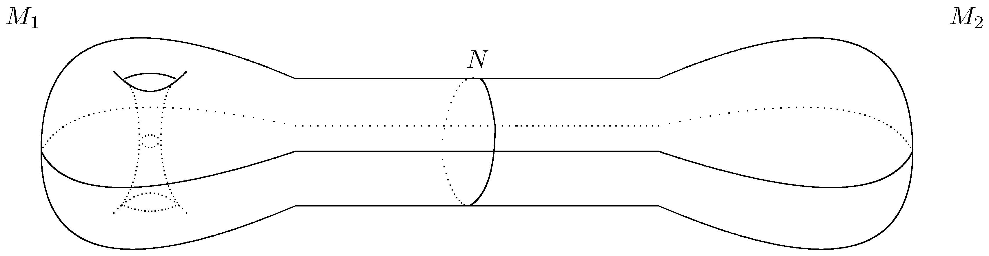
Let $(M,g)$ be an $(m+1)$-dimensional compact oriented Riemannian manifold. Furthermore, let N be a compact hypersurface of M, so that the closure of $M-N$ has two components, $M_1$ and $M_2$. The manifold M therefore consists of the manifolds $M_1$ and $M_2$ glued together; see Figure 1. It is a natural question to ask if there are relationships between spectral quantities on $M_1$, $M_2$, and the manifold $M=M_1{\cup }_N{M}_2$ obtained when gluing them together. For a particular spectral quantity, the BFK-gluing formula sheds some light on this question.

Remark 1.

The assumption for the gluing formula to hold is that $\partial N=\varnothing$. In Figure 1, this means M is a two-dimensional surface and N is a circle. We come back to this assumption in the conclusions, providing an example in which the BFK-gluing formula holds despite that $\partial N\ne \varnothing$.

In order to formulate the BFK-gluing formula, let ${\Delta }_M$ denote the Laplacian acting on smooth functions, and denote by ${\Delta }_{M_1,D}$ and ${\Delta }_{M_2,D}$ the restriction of ${\Delta }_M$ to $M_1$, $M_2$ with Dirichlet boundary conditions imposed on N. In the case that $\partial M\ne \varnothing$, we also impose Dirichlet boundary conditions on $\partial M$. Let ${\alpha }_j$, ${\alpha }_{1,j}$ and ${\alpha }_{2,j}$ be the eigenvalues of ($0\le \lambda \in \mathbf{R}$):

$$\begin{array}{ccc}\hfill ({\Delta }_M+\lambda )u_j\left(x\right)& =& {\alpha }_j{u}_j\left(x\right),\hfill \\ \hfill ({\Delta }_{M_1,D}+\lambda )v_j\left(x\right)& =& {\left.{\alpha }_{1,j}{v}_j\left(x\right),v_j\left(x\right)\right|}_N=0\hfill \\ \hfill ({\Delta }_{M_2,D}+\lambda )w_j\left(x\right)& =& {\left.{\alpha }_{2,j}{w}_j\left(x\right),w_j\left(x\right)\right|}_N=0\hfill \end{array}$$

We denote the associated zeta functions by ${\zeta }_M\left(s\right)$, ${\zeta }_{M_1,D}\left(s\right)$ and ${\zeta }_{M_2,D}\left(s\right)$ and have the standard definitions:

$${\zeta }_M\left(s\right)=\sum _{j=1}^{\infty }{\alpha }_j^{-s},{\zeta }_{M_1,D}\left(s\right)=\sum _{j=1}^{\infty }{\alpha }_{1,j}^{-s},{\zeta }_{M_2,D}\left(s\right)=\sum _{j=1}^{\infty }{\alpha }_{2,j}^{-s}$$

In case there is a zero mode on M, for example ${\alpha }_0=0$, it is excluded in the summation. These zeta functions are meromorphic functions in the complex plane, and in particular they are analytic about $s=0$; ${\zeta }_M^{\prime }\left(0\right)$, ${\zeta }_{M_1,D}^{\prime }\left(0\right)$, ${\zeta }_{M_2,D}^{\prime }\left(0\right)$ are well-defined quantities [33] that one defines the associated determinants through:

$$ln\mathrm{Det}P=-{\zeta }_P^{\prime }\left(0\right)$$

These quantities make up the left-hand side (LHS) of the BFK-gluing formula. A relation to quantum field theory is established by choosing the manifolds M, $M_1$, and $M_2$ to have the product structures $M=\mathcal{M}\times S^1$, $M_1={\mathcal{M}}_1\times S^1$, and $M_2={\mathcal{M}}_2\times S^1$, where $S^1$ is a circle of perimeter $\beta$. In this case, these quantities are the partition sums for a finite-temperature quantum field theory at temperature $1/\beta$ of a non-interacting massive scalar field living on $\mathcal{M}$, ${\mathcal{M}}_1$, and ${\mathcal{M}}_2$; see Section 3. The remaining ingredient for the BFK-gluing formula is the Dirichlet-to-Neumann operator. Let ${\partial }_N$ be a unit normal vector field to N such that it points outward on $M_1$ and inward on $M_2$. The Dirichlet-to-Neumann operator $R\left(\lambda \right):C^{\infty }\left(N\right)\to C^{\infty }\left(N\right)$ is then defined as follows. For $h\in C^{\infty }\left(N\right)$, let ${\varphi }_1\in C^{\infty }\left(M_1\right)$ and ${\varphi }_2\in C^{\infty }\left(M_2\right)$ be such that

$$({\Delta }_{M_1}+\lambda ){\varphi }_1=0,({\Delta }_{M_2}+\lambda ){\varphi }_2=0,{\varphi }_1{\left|{}_N={\varphi }_2\right|}_N=h$$

(1)

We then define

$$R\left(\lambda \right)h:=\left({\partial }_N{\varphi }_1\right){\left|{}_N-\left({\partial }_N{\varphi }_2\right)\right|}_N$$

(2)

This specifies an elliptic pseudodifferential operator of order 1; the associated zeta function ${\zeta }_{DN}\left(s\right)$ is regular at $s=0$, and ${\zeta }_{DN}^{\prime }\left(0\right)$ is again well defined [31,33].

The BFK-gluing formula relates these quantities through a polynomial:

$$P\left(\lambda \right)=\sum _{j=0}^{\left[\frac{m}{2}\right]}{p}_j{\lambda }^j$$

which is determined as an integral of some local density on N and which is completely determined by data on a collared neighborhood of N. In detail, we have

$$ln\mathrm{Det}({\Delta }_M+\lambda )-ln\mathrm{Det}({\Delta }_{M_1,D}+\lambda )-ln\mathrm{Det}({\Delta }_{M_2,D}+\lambda )=P\left(\lambda \right)+ln\mathrm{Det}R\left(\lambda \right)$$

(3)

or using zeta functions instead,

$$-{\zeta }_M^{\prime }\left(0\right)+{\zeta }_{M_1,D}^{\prime }\left(0\right)+{\zeta }_{M_2,D}^{\prime }\left(0\right)=P\left(\lambda \right)-{\zeta }_{DN}^{\prime }\left(0\right)$$

(4)

If zero modes are present, slight modifications to Equation (3) occur [30], which will, however, be irrelevant for our application.

Given this is the basis of everything that follows, for a self-contained presentation, we include the proof of this statement for zeta-determinants of Laplacians on a compact or complete Riemannian manifold given in [30].

The underlying idea to prove Equation (3) is that by taking $[m/2]+1$ derivatives on both sides, equality of both sides is obtained. For the formulation of the proof, we introduce some notation. As before, let $(M,g)$ be a complete oriented $(m+1)$-dimensional Riemannian manifold with a compact hypersurface N. We denote by $M_0$ the closure of $M-N$ so that $(M_0,g_0)$ is a Riemannian manifold with boundary $N^{+}\cup N^{-}$, where $g_0$ is a metric induced from g and $N^{+}=N^{-}=N$. We here note that $M_0$ may or may not be connected. Furthermore, as before, we denote by ${\Delta }_M$ a Laplacian acting on $C^{\infty }\left(M\right)$, and by ${\Delta }_{M_0,D}$, the extension of ${\Delta }_M$ to $M_0$ with the Dirichlet boundary condition on $N^{+}\cup N^{-}$. By a Laplacian, we mean a symmetric non-negative differential operator of order 2 with the principal symbol ${\sigma }_L\left({\Delta }_M\right)(x,\xi )=\parallel \xi \parallel {}^2$ satisfying the property of the finite propagation speed (FPS). It is shown in [34] that ${\Delta }_M$ is essentially self-adjoint. Furthermore, we assume that ${\Delta }_{M_0,D}$ is a non-negative invertible operator. These assumptions show that for $\lambda \in {\mathbb{R}}^{+}\cup \left\{0\right\}$, ${({\Delta }_M+\lambda )}^{-1}$ and ${({\Delta }_{M_0,D}+\lambda )}^{-1}$ are bounded operators defined on $L^2\left(M\right)$. In many cases, operators arising from geometry satisfy these assumptions [35,36,37].

It is known (p 327 of [31]; see also [38]) that $e^{-t{\Delta }_M}-e^{-t{\Delta }_{M_0,D}}$ is a trace-class operator and that for $t\to 0^{+}$,

$$\begin{array}{ccc}\hfill Tr\left(e^{-t{\Delta }_M}-e^{-t{\Delta }_{M_0,D}}\right)& \sim & \sum _{j=0}^{\infty }{a}_j{t}^{-\frac{m-j}{2}}\hfill \end{array}$$

(5)

where $a_j\in \mathbb{R}$. Because $Tr\left(e^{-t{\Delta }_M}-e^{-t{\Delta }_{M_0,D}}\right)$ is a trace-class operator and ${\Delta }_{M_0,D}$ is an invertible operator, the dimension of the kernel of ${\Delta }_M$ is finite. Hence Theorem 2.2 of [39] tells that for some $c>0$ as $t\to \infty$, we have

$$\begin{array}{ccc}\hfill Tr\left(e^{-t{\Delta }_M}-e^{-t{\Delta }_{M_0,D}}\right)& =& dimker{\Delta }_M+O\left(e^{-ct}\right)\hfill \end{array}$$

(6)

This shows that for $\lambda \in {\mathbb{R}}^{+}$,

$$\begin{array}{c}\hfill Tr\left(e^{-t({\Delta }_M+\lambda )}-e^{-t({\Delta }_{M_0,D}+\lambda )}\right)\end{array}$$

(7)

is exponentially decreasing for $t\to \infty$. We note that

$$\begin{array}{c}\hfill \begin{array}{c}{\int }_t^{\infty }\left(e^{-u({\Delta }_M+\lambda )}-e^{-u({\Delta }_{M_0,D}+\lambda )}\right)du\hfill \\ ={({\Delta }_M+\lambda )}^{-1}{e}^{-t({\Delta }_M+\lambda )}-{({\Delta }_{M_0,D}+\lambda )}^{-1}{e}^{-t({\Delta }_{M_0,D}+\lambda )}\hfill \end{array}\end{array}$$

(8)

This shows that ${({\Delta }_M+\lambda )}^{-1}{e}^{-t({\Delta }_M+\lambda )}-{({\Delta }_{M_0,D}+\lambda )}^{-1}{e}^{-t({\Delta }_{M_0,D}+\lambda )}$ is a trace-class operator and

$$\begin{array}{c}\hfill \begin{array}{c}Tr\left({({\Delta }_M+\lambda )}^{-1}{e}^{-t({\Delta }_M+\lambda )}-{({\Delta }_{M_0,D}+\lambda )}^{-1}{e}^{-t({\Delta }_{M_0,D}+\lambda )}\right)\hfill \\ \sim \left\{\begin{array}{cc}{\sum }_{j=0}^{m-3}\frac{{\tilde{a}}_j}{\frac{m-j}{2}-1}{t}^{-\frac{m-j}{2}+1}+{\tilde{a}}_{m-2}lnt+O\left(1\right)\hfill & \mathrm{for}t\to 0^{+}\hfill \\ O\left(e^{-ct}\right)\hfill & \mathrm{for}t\to \infty \hfill \end{array}\right.\hfill \end{array}\end{array}$$

(9)

where

$$Tr\left(e^{-t({\Delta }_M+\lambda )}-e^{-t({\Delta }_{M_0,D}+\lambda )}\right)\sim \sum _{j=0}^{\infty }{\tilde{a}}_j{t}^{-\frac{m-j}{2}}$$

If we repeat this argument, after $\nu =\left[\frac{m}{2}\right]+1$ integrations, we have for some $\tilde{c}>0$ that

$$\begin{array}{ccc}\hfill Tr\left({({\Delta }_M+\lambda )}^{-\nu }{e}^{-t({\Delta }_M+\lambda )}-{({\Delta }_{M_0,D}+\lambda )}^{-\nu }{e}^{-t({\Delta }_{M_0,D}+\lambda )}\right)& \sim & \left\{\begin{array}{cc}O\left(1\right)\hfill & \mathrm{for}t\to 0^{+}\hfill \\ O\left(e^{-\tilde{c}t}\right)\hfill & \mathrm{for}t\to \infty \hfill \end{array}\right.\hfill \end{array}$$

(10)

Similarly, it can be shown that for $t\to 0^{+}$,

$$\begin{array}{c}\hfill \begin{array}{c}Tr\left({({\Delta }_M+\lambda )}^{-\nu +1}{e}^{-t({\Delta }_M+\lambda )}-{({\Delta }_{M_0,D}+\lambda )}^{-\nu +1}{e}^{-t({\Delta }_{M_0,D}+\lambda )}\right)\hfill \\ \sim \left\{\begin{array}{cc}O(lnt)\hfill & \mathrm{for}m\mathrm{even}\hfill \\ O\left(t^{-\frac{1}{2}}\right)\hfill & \mathrm{for}m\mathrm{odd}\hfill \end{array}\right.\hfill \end{array}\end{array}$$

(11)

and hence

$$\begin{array}{c}\hfill {\int }_0^{\infty }Tr\left({({\Delta }_M+\lambda )}^{-\nu +1}{e}^{-t({\Delta }_M+\lambda )}-{({\Delta }_{M_0,D}+\lambda )}^{-\nu +1}{e}^{-t({\Delta }_{M_0,D}+\lambda )}\right)dt\end{array}$$

(12)

is integrable.

Taking the limit $t\to 0^{+}$ in Equation (10), this leads to the following result.

Lemma 1.

${({\Delta }_M+\lambda )}^{-\nu }-{({\Delta }_{M_0,D}+\lambda )}^{-\nu }$ is a trace-class operator.

We define a relative zeta function by

$$\begin{array}{c}\hfill \begin{array}{ccc}\hfill \zeta (s;{\Delta }_M+\lambda ,{\Delta }_{M_0,D}+\lambda )& =& \frac{1}{\mathsf{\Gamma }\left(s\right)}{\int }_0^{\infty }{t}^{s-1}Tr\left(e^{-t({\Delta }_M+\lambda )}-e^{-t({\Delta }_{M_0,D}+\lambda )}\right)dt\hfill \\ & =& \frac{1}{\mathsf{\Gamma }\left(s\right)}{\int }_0^{\infty }{t}^{s-1}{e}^{-\lambda t}Tr\left(e^{-t{\Delta }_M}-e^{-t{\Delta }_{M_0,D}}\right)dt\hfill \end{array}\end{array}$$

(13)

It is well known that $\zeta (s;{\Delta }_M+\lambda ,{\Delta }_{M_0,D}+\lambda )$ is analytic for $\mathrm{Re}s>\frac{m}{2}$ and has an analytic continuation to the whole complex plane, having a regular value at $s=0$. We define the relative zeta-determinant by

$$\begin{array}{c}\hfill {\left.lnDet\left({\Delta }_M+\lambda ,{\Delta }_{M_0,D}+\lambda \right)=-\frac{d}{ds}\right|}_{s=0}\zeta (s;{\Delta }_M+\lambda ,{\Delta }_{M_0,D}+\lambda )\end{array}$$

(14)

For general facts about the relative zeta-determinant, we refer to [39].

Lemma 2.

For $\lambda >0$, we have the following equality:

$$\begin{array}{ccc}\hfill \frac{d^{\nu }}{d{\lambda }^{\nu }}lnDet\left({\Delta }_M+\lambda ,{\Delta }_{M_0,D}+\lambda \right)& =& Tr\left\{\frac{d^{\nu -1}}{d{\lambda }^{\nu -1}}\left({({\Delta }_M+\lambda )}^{-1}-{({\Delta }_{M_0,D}+\lambda )}^{-1}\right)\right\}\hfill \end{array}$$

Proof. 

We note that for $\mathrm{Re}s>\frac{m}{2}$,

$$\begin{array}{cc}& \frac{d^{\nu }}{d{\lambda }^{\nu }}\zeta (s;{\Delta }_M+\lambda ,{\Delta }_{M_0,D}+\lambda )=\frac{{(-1)}^{\nu }}{\mathsf{\Gamma }\left(s\right)}{\int }_0^{\infty }{t}^{s+\nu -1}Tr\left(e^{-t({\Delta }_M+\lambda )}-e^{-t({\Delta }_{M_0,D}+\lambda )}\right)dt\hfill \\ =& \frac{{(-1)}^{\nu }}{\mathsf{\Gamma }\left(s\right)}{\int }_0^{\infty }{t}^{s+\nu -1}\left(-\frac{d}{dt}\right)Tr\left\{{({\Delta }_M+\lambda )}^{-1}{e}^{-t({\Delta }_M+\lambda )}-{({\Delta }_{M_0,D}+\lambda )}^{-1}{e}^{-t({\Delta }_{M_0,D}+\lambda )}\right\}dt\hfill \\ =& \frac{{(-1)}^{\nu }(s+\nu -1)}{\mathsf{\Gamma }\left(s\right)}{\int }_0^{\infty }{t}^{s+\nu -2}Tr\left\{{({\Delta }_M+\lambda )}^{-1}{e}^{-t({\Delta }_M+\lambda )}-{({\Delta }_{M_0,D}+\lambda )}^{-1}{e}^{-t({\Delta }_{M_0,D}+\lambda )}\right\}dt\hfill \\ =& \frac{{(-1)}^{\nu }(s+\nu -1)\cdots (s+1)}{\mathsf{\Gamma }\left(s\right)}\hfill \\ & \times {\int }_0^{\infty }{t}^{s}Tr\left\{{({\Delta }_M+\lambda )}^{-\nu +1}{e}^{-t({\Delta }_M+\lambda )}-{({\Delta }_{M_0,D}+\lambda )}^{-\nu +1}{e}^{-t({\Delta }_{M_0,D}+\lambda )}\right\}dt\hfill \end{array}$$

Using Equations (11) and (12) together with Equation (14), we have

$$\begin{array}{cc}& \frac{d^{\nu }}{d{\lambda }^{\nu }}lnDet\left({\Delta }_M+\lambda ,{\Delta }_{M_0,D}+\lambda \right)=-\frac{d}{ds}{|}_{s=0}\frac{d^{\nu }}{d{\lambda }^{\nu }}\zeta (s;{\Delta }_M+\lambda ,{\Delta }_{M_0,D}+\lambda )\hfill \\ =& -{(-1)}^{\nu }(\nu -1)!{\int }_0^{\infty }Tr\left\{{({\Delta }_M+\lambda )}^{-\nu +1}{e}^{-t({\Delta }_M+\lambda )}-{({\Delta }_{M_0,D}+\lambda )}^{-\nu +1}{e}^{-t({\Delta }_{M_0,D}+\lambda )}\right\}dt\hfill \\ =& -{(-1)}^{\nu }(\nu -1)!{\int }_0^{\infty }\left(-\frac{d}{dt}\right)Tr\left\{{({\Delta }_M+\lambda )}^{-\nu }{e}^{-t({\Delta }_M+\lambda )}-{({\Delta }_{M_0,D}+\lambda )}^{-\nu }{e}^{-t({\Delta }_{M_0,D}+\lambda )}\right\}dt\hfill \\ =& {(-1)}^{\nu -1}(\nu -1)!Tr\left\{{({\Delta }_M+\lambda )}^{-\nu }-{({\Delta }_{M_0,D}+\lambda )}^{-\nu }\right\}\hfill \\ =& Tr\left\{\frac{d^{\nu -1}}{d{\lambda }^{\nu -1}}\left({({\Delta }_M+\lambda )}^{-1}-{({\Delta }_{M_0,D}+\lambda )}^{-1}\right)\right\}\hfill \end{array}$$

☐

We next analyze the Dirichlet-to-Neumann operator $R\left(\lambda \right):C^{\infty }\left(N\right)\to C^{\infty }\left(N\right)$ as follows. For this purpose, we need to define some auxiliary operators. We recall that the boundary of $M_0$ is $N^{+}\cup N^{-}$. We choose a unit normal vector field ${\partial }_N$ along N, which points outward on $N^{+}$ and inward on $N^{-}$. We define ${\delta }_{diag}:C^{\infty }\left(N\right)\to C^{\infty }(N^{+}\cup N^{-})$ and $C:C^{\infty }\left(M_0\right)\to C^{\infty }\left(N\right)$ as follows:

$$\begin{array}{c}\hfill \begin{array}{c}{\delta }_{diag}:C^{\infty }\left(N\right)\to C^{\infty }(N^{+}\cup N^{-}){\delta }_{diag}\left(f\right)=(f,f),\hfill \\ C:C^{\infty }\left(M_0\right)\to C^{\infty }\left(N\right),C\left(\varphi \right)=\left({\partial }_N\varphi \right){{|}_{N^{+}}-\left({\partial }_N\varphi \right)|}_{N^{-}}\hfill \end{array}\end{array}$$

(15)

For later use, we define the restriction maps ${\gamma }_0$ and ${\tilde{\gamma }}_0$ as follows:

$$\begin{array}{c}\hfill \begin{array}{c}{\gamma }_0:C^{\infty }\left(M\right)\to C^{\infty }\left(N\right),{\gamma }_0{\varphi =\varphi |}_N,\hfill \\ {\tilde{\gamma }}_0:C^{\infty }\left(M_0\right)\to C^{\infty }\left(N^{+}\right)\oplus C^{\infty }\left(N^{-}\right){\tilde{\gamma }}_0\psi ={\left(\psi \right|}_{N^{+}},\psi {|}_{N^{-}})\hfill \end{array}\end{array}$$

(16)

Finally, we define the Poisson operator ${\mathcal{P}}_D\left(\lambda \right):C^{\infty }\left(N^{+}\right)\oplus C^{\infty }\left(N^{-}\right)\to C^{\infty }\left(M_0\right)$ as follows. For $(f,g)\in C^{\infty }\left(N^{+}\right)\oplus C^{\infty }\left(N^{-}\right)$, we choose $\psi \in C^{\infty }\left(M_0\right)$ satisfying

$$\begin{array}{c}\hfill ({\Delta }_{M_0}+\lambda )\psi =0,{\tilde{\gamma }}_0\psi =(f,g)\end{array}$$

(17)

In fact, $\psi$ is given by

$$\begin{array}{c}\hfill \psi :=\tilde{f}-{({\Delta }_{M_0,D}+\lambda )}^{-1}({\Delta }_M+\lambda )\tilde{f}\end{array}$$

(18)

where $\tilde{f}$ is an arbitrary extension of $(f,g)$ to $M_0$. Because ${\Delta }_{M_0,D}+\lambda$ is an invertible operator, $\psi$ exists uniquely. We then define the Poisson operator ${\mathcal{P}}_D\left(\lambda \right)$ by

$$\begin{array}{c}\hfill {\mathcal{P}}_D\left(\lambda \right):C^{\infty }\left(N^{+}\right)\oplus C^{\infty }\left(N^{-}\right)\to C^{\infty }\left(M_0\right),{\mathcal{P}}_D\left(\lambda \right)(f,g)=\psi \end{array}$$

(19)

Using the above operators, the Dirichlet-to-Neumann operator $R\left(\lambda \right)$ defined in Equations (1) and (2) is then reformulated as follows.

Definition 1.

$R\left(\lambda \right):C^{\infty }\left(N\right)\to C^{\infty }\left(N\right),R\left(\lambda \right)=C·{\mathcal{P}}_D\left(\lambda \right)·{\delta }_{diag}$

where “·” means the composition of operators.

We need the following two auxiliary lemmas.

Lemma 3.

$\frac{d}{d\lambda }{\mathcal{P}}_D\left(\lambda \right)=-{\left({\Delta }_{M_0,D}+\lambda \right)}^{-1}{\mathcal{P}}_D\left(\lambda \right)$

Proof. 

From the definition of the Poisson operator, ${\mathcal{P}}_D\left(\lambda \right)$ satisfies the following two equalities:

$$\begin{array}{c}\hfill \left({\Delta }_{M_0}+\lambda \right){\mathcal{P}}_D\left(\lambda \right)=0,{\tilde{\gamma }}_0{\mathcal{P}}_D\left(\lambda \right)=Id\end{array}$$

Taking the derivative with respect to $\lambda$, from here we have

$$\begin{array}{c}\hfill {\mathcal{P}}_D\left(\lambda \right)+\left({\Delta }_{M_0}+\lambda \right)\frac{d}{d\lambda }{\mathcal{P}}_D\left(\lambda \right)=0,{\tilde{\gamma }}_0\frac{d}{d\lambda }{\mathcal{P}}_D\left(\lambda \right)=0\end{array}$$

which shows that $\frac{d}{d\lambda }{\mathcal{P}}_D\left(\lambda \right)=-{\left({\Delta }_{M_0,D}+\lambda \right)}^{-1}{\mathcal{P}}_D\left(\lambda \right)$. ☐

We note that ${\left({\Delta }_M+\lambda \right)}^{-1}:L^2\left(M\right)\to L^2\left(M\right)$ and ${\left({\Delta }_{M_0,D}+\lambda \right)}^{-1}:L^2\left(M_0\right)\to L^2\left(M_0\right)$ are bounded operators and $L^2\left(M_0\right)$ can be identified with $L^2\left(M\right)$. Hence, ${\left({\Delta }_{M_0,D}+\lambda \right)}^{-1}$ can be regarded as an operator acting on $L^2\left(M\right)$. The next lemma shows the relation between the two operators.

Lemma 4.

${\left({\Delta }_M+\lambda \right)}^{-1}-{\left({\Delta }_{M_0,D}+\lambda \right)}^{-1}={\mathcal{P}}_D\left(\lambda \right)·{\delta }_{diag}·{\gamma }_0·{\left({\Delta }_M+\lambda \right)}^{-1}.$

Proof. 

Because the operators on the LHS and right-hand side (RHS) are bounded, it is enough to check the equality on $C^{\infty }\left(M\right)$ in $L^2\left(M\right)$. Let $A\left(\lambda \right):={\left({\Delta }_M+\lambda \right)}^{-1}-{\left({\Delta }_{M_0,D}+\lambda \right)}^{-1}$. For $\varphi \in C^{\infty }\left(M\right)$,

$$\begin{array}{c}\hfill \left({\Delta }_M+\lambda \right)A\left(\lambda \right)\varphi =0,{\gamma }_{0}A\left(\lambda \right)\varphi ={\gamma }_0{\left({\Delta }_M+\lambda \right)}^{-1}\varphi \end{array}$$

which shows that $A\left(\lambda \right)={\mathcal{P}}_D\left(\lambda \right)·{\delta }_{diag}·{\gamma }_0·{\left({\Delta }_M+\lambda \right)}^{-1}$. ☐

From Definition 1 and Lemmas 3 and 4, we then have the following equalities:

$$\begin{array}{c}\hfill \begin{array}{ccc}\hfill \frac{d}{d\lambda }R\left(\lambda \right)& =& C·\frac{d}{d\lambda }{\mathcal{P}}_D\left(\lambda \right)·{\delta }_{diag}\hfill \\ & =& -C·{\left({\Delta }_{M_0,D}+\lambda \right)}^{-1}{\mathcal{P}}_D\left(\lambda \right)·{\delta }_{diag}\hfill \\ & =& C·\left\{-{\left({\Delta }_M+\lambda \right)}^{-1}+{\mathcal{P}}_D\left(\lambda \right)·{\delta }_{diag}·{\gamma }_0·{\left({\Delta }_M+\lambda \right)}^{-1}\right\}·{\mathcal{P}}_D\left(\lambda \right)·{\delta }_{diag}\hfill \\ & =& -C·{\left({\Delta }_M+\lambda \right)}^{-1}·{\mathcal{P}}_D\left(\lambda \right)·{\delta }_{diag}+C·{\mathcal{P}}_D\left(\lambda \right)·{\delta }_{diag}·{\gamma }_0·{\left({\Delta }_M+\lambda \right)}^{-1}·\hfill \\ & & {\mathcal{P}}_D\left(\lambda \right)·{\delta }_{diag}\hfill \end{array}\end{array}$$

(20)

Lemma 5.

$C·{\left({\Delta }_M+\lambda \right)}^{-1}·{\mathcal{P}}_D\left(\lambda \right)·{\delta }_{diag}:L^2\left(N\right)\to L^2\left(N\right)$ is a zero operator.

Proof. 

Because $C·{\left({\Delta }_M+\lambda \right)}^{-1}·{\mathcal{P}}_D\left(\lambda \right)·{\delta }_{diag}$ is a bounded operator, it is enough to check on $C^{\infty }\left(M\right)$ in $L^2\left(M\right)$. For $f\in C^{\infty }\left(N\right)$, ${\mathcal{P}}_D\left(\lambda \right)·{\delta }_{diag}f$ is continuous and ${\left({\Delta }_M+\lambda \right)}^{-1}·{\mathcal{P}}_D\left(\lambda \right)·{\delta }_{diag}f\in H^2\left(M\right)$; hence $C·{\left({\Delta }_M+\lambda \right)}^{-1}·{\mathcal{P}}_D\left(\lambda \right)·{\delta }_{diag}f=0$. ☐

From the above lemma, we have the following equalities:

$$\begin{array}{c}\hfill \begin{array}{ccc}\hfill \frac{d}{d\lambda }R\left(\lambda \right)& =& C·{\mathcal{P}}_D\left(\lambda \right)·{\delta }_{diag}·{\gamma }_0·{\left({\Delta }_M+\lambda \right)}^{-1}·{\mathcal{P}}_D\left(\lambda \right)·{\delta }_{diag}\hfill \\ & =& R\left(\lambda \right)·{\gamma }_0·{\left({\Delta }_M+\lambda \right)}^{-1}·{\mathcal{P}}_D\left(\lambda \right)·{\delta }_{diag}\hfill \end{array}\end{array}$$

(21)

which shows that

$$\begin{array}{c}\hfill \begin{array}{ccc}\hfill R{\left(\lambda \right)}^{-1}·\frac{d}{d\lambda }R\left(\lambda \right)& =& {\gamma }_0·{\left({\Delta }_M+\lambda \right)}^{-1}·{\mathcal{P}}_D\left(\lambda \right)·{\delta }_{diag}\hfill \\ & =& {\gamma }_0·\left\{{\left({\Delta }_M+\lambda \right)}^{-1}-{\left({\Delta }_{M_0,D}+\lambda \right)}^{-1}\right\}·{\mathcal{P}}_D\left(\lambda \right)·{\delta }_{diag}\hfill \\ & =& {\gamma }_0·\left\{{\mathcal{P}}_D\left(\lambda \right)·{\delta }_{diag}·{\gamma }_0·{\left({\Delta }_M+\lambda \right)}^{-1}\right\}·{\mathcal{P}}_D\left(\lambda \right)·{\delta }_{diag}\hfill \\ & =& {\gamma }_0·{\left({\Delta }_M+\lambda \right)}^{-1}·{\mathcal{P}}_D\left(\lambda \right)·{\delta }_{diag}\hfill \end{array}\end{array}$$

(22)

where we have used the fact that ${\gamma }_0·{\mathcal{P}}_D\left(\lambda \right)·{\delta }_{diag}=Id$. Lemmas 2 and 4 then finally yield the following equality:

$$\begin{array}{c}\hfill \begin{array}{ccc}\hfill \frac{d^{\nu }}{d{\lambda }^{\nu }}lnDet\left({\Delta }_M+\lambda ,{\Delta }_{M_0,D}+\lambda \right)& =& Tr\left\{\frac{d^{\nu -1}}{d{\lambda }^{\nu -1}}\left({({\Delta }_M+\lambda )}^{-1}-{({\Delta }_{M_0,D}+\lambda )}^{-1}\right)\right\}\hfill \\ & =& Tr\left\{\frac{d^{\nu -1}}{d{\lambda }^{\nu -1}}\left({\mathcal{P}}_D\left(\lambda \right)·{\delta }_{diag}·{\gamma }_0·{\left({\Delta }_M+\lambda \right)}^{-1}\right)\right\}\hfill \\ & =& Tr\left\{\frac{d^{\nu -1}}{d{\lambda }^{\nu -1}}\left({\gamma }_0·{\left({\Delta }_M+\lambda \right)}^{-1}·{\mathcal{P}}_D\left(\lambda \right)·{\delta }_{diag}\right)\right\}\hfill \\ & =& Tr\left\{\frac{d^{\nu -1}}{d{\lambda }^{\nu -1}}\left(R{\left(\lambda \right)}^{-1}·\frac{d}{d\lambda }R\left(\lambda \right)\right)\right\}\hfill \\ & =& \frac{d^{\nu }}{d{\lambda }^{\nu }}lnDetR\left(\lambda \right)\hfill \end{array}\end{array}$$

(23)

where in the third step, cyclicity of the trace has been used.

Summarizing the above argument, we have shown the BFK-gluing formula in the context of Laplace-type operators.

Theorem 1.

There exists a real polynomial $P\left(\lambda \right)$ of degree less than or equal to $\left[\frac{m}{2}\right]$ such that

$$\begin{array}{ccc}\hfill lnDet\left({\Delta }_M+\lambda ,{\Delta }_{M_0,D}+\lambda \right)& =& P\left(\lambda \right)+lnDetR\left(\lambda \right)\hfill \end{array}$$

where $P\left(\lambda \right)={\sum }_{j=0}^{\left[\frac{m}{2}\right]}{p}_j{\lambda }^j$.

This is equivalent to Equations (3) and (4). The fact that $p_j$ is given as an integral of some density on N follows from the $\lambda \to \infty$ behavior of $lnDet\left({\Delta }_M+\lambda ,{\Delta }_{M_0,D}+\lambda \right)$ and $lnDetR\left(\lambda \right)$ [30].

Example 1.

As an illustration, we consider a simple one-dimensional example. Let $0<c<1$ and $I_c=[0,c]$. The setting for the gluing formula is $I_1=I_c{\cup }_{\left\{c\right\}}[c,1]$. We consider the following eigenvalue problem:

$$-\frac{{\partial }^2}{\partial x^2}{\varphi }_n\left(x\right)={\lambda }_n{\varphi }_n\left(x\right),{\varphi }_n\left(0\right)={\varphi }_n\left(c\right)=0$$

The eigenfunctions and eigenvalues then are

$${\varphi }_n\left(x\right)=sin\left(\frac{n\pi x}{c}\right),{\lambda }_n={\left(\frac{n\pi }{c}\right)}^2,n\in \mathbf{N}$$

and the associated zeta function is given by the zeta function ${\zeta }_R\left(s\right)$ of Riemann. In detail,

$${\zeta }_c\left(s\right)={\left(\frac{c}{\pi }\right)}^{2s}{\zeta }_R\left(2s\right)$$

and thus

$${\zeta }_c^{\prime }\left(0\right)=-ln\left(2c\right)$$

Similarly the intervals $[c,1]$ and $I_1$ can be treated and the relevant combination on the LHS of Theorem 1 then is

$$-{\zeta }_1^{\prime }\left(0\right)+{\zeta }_c^{\prime }\left(0\right)+{\zeta }_{1-c}^{\prime }\left(0\right)=-ln\left[2c(1-c)\right]$$

On the other side, the Dirichlet-to-Neumann map involves the solutions to the following problems:

$$\begin{array}{c}\frac{{\partial }^2}{\partial x^2}{\psi }_1\left(x\right)=0,{\psi }_1\left(0\right)=0,{\psi }_1\left(c\right)=h\\ \frac{{\partial }^2}{\partial x^2}{\psi }_2\left(x\right)=0,{\psi }_2\left(1\right)=0,{\psi }_2\left(c\right)=h\end{array}$$

In terms of these, one defines

$$R\left(h\right)={\left.\frac{\partial }{\partial x}\left({\psi }_1-{\psi }_2\right)\right|}_{x=c}$$

Explicitly, it is easy to see that

$${\psi }_1\left(x\right)=\frac{h}{c}x,{\psi }_2\left(x\right)=\frac{h}{1-c}(1-x)$$

such that

$$R\left(h\right)=\frac{h}{c}+\frac{h}{1-c}=\frac{h}{c(1-c)}$$

and

$$ln\mathrm{Det}R=-ln\left[c(1-c)\right]$$

For this example, we therefore verify that Theorem 1 is satisfied with

$$P\left(0\right)=-ln2$$

3. Gluing Formula for Casimir Energies

We next relate the gluing formula to a finite-temperature quantum field theory of a non-self-interacting massive scalar field in a piston geometry. Relevant one-particle energy spectra then follow from eigenvalues of suitable Laplace-type operators. As indicated earlier, to relate this quantum field theory to the considerations of Section 2, let $M_i={\mathcal{M}}_i\times S^1$, where $S^1$ denotes a circle of perimeter $\beta$, and ${\mathcal{M}}_i$ denotes a smooth compact Riemannian manifold with smooth boundary $\mathcal{N}$. This manifold represents the spatial dimensions of the space-time where the quantum field lives. As far as Figure 1 goes, what one sees there is really ${\mathcal{M}}_1$ and ${\mathcal{M}}_2$, although for the application to the gluing formula, $M_i={\mathcal{M}}_i\times S^1$ is needed.

Let $\tau \in [0,\beta ]$ parameterize $S^1$ and impose periodic boundary conditions along that circle. Furthermore, let y be coordinates on ${\mathcal{M}}_i$. For the analysis of Casimir energies, the relevant eigenvalue problems then are, with $\lambda$ being the mass of the quantum field,

$${\left.\left({\Delta }_{M_i,D}+\lambda \right){\varphi }_{j,n}^{\left(i\right)}(\tau ,y)={\alpha }_{j,n}^{\left(i\right)}{\varphi }_{j,n}^{\left(i\right)}(\tau ,y),{\varphi }_{j,n}^{\left(i\right)}(\tau ,y)\right|}_{y\in \mathcal{N}}=0$$

(24)

More explicitly, because of the product structure,

$${\alpha }_{j,n}^{\left(i\right)}={\left(\frac{2\pi n}{\beta }\right)}^2+E_{i,j}^2,n\in \mathbf{Z},j\in \mathbf{N}$$

(25)

where $E_{i,j}^2$ are the eigenvalues of the “spatial part” of the Laplacian, namely we have

$${\left.\left({\Delta }_{{\mathcal{M}}_i,D}+\lambda \right){\phi }_j^{\left(i\right)}\left(y\right)=E_{i,j}^2{\phi }_j^{\left(i\right)}\left(y\right),{\phi }_j^{\left(i\right)}\left(y\right)\right|}_{y\in \mathcal{N}}=0$$

(26)

The associated zeta functions,

$${\zeta }^{\left(i\right)}\left(s\right)=\sum _{n=-\infty }^{\infty }\sum _{j=1}^{\infty }{\left[{\left(\frac{2\pi n}{\beta }\right)}^2+E_{i,j}^2\right]}^{-s}$$

(27)

encode the finite-temperature Casimir energy via

$$E_{Cas}^{\left(i\right)}=-\frac{1}{2}\frac{\partial }{\partial \beta }{{\zeta }^{\left(i\right)}}^{\prime }\left(0\right)$$

(28)

Leaving a discussion of finite ambiguities aside, when discussing forces, there will be none; it is an interesting question to ask how the Casimir energy behaves when gluing together two manifolds with identical boundaries. More precisely, the question is what the relation is between $E_{Cas}$, the Casimir energy on $M=\mathcal{M}\times S^1$, and $E_{Cas}^{\left(1\right)}+E_{Cas}^{\left(2\right)}$. An answer is provided by the gluing formula; namely from Equation (4), one has

$$E_{Cas}-E_{Cas}^{\left(1\right)}-E_{Cas}^{\left(2\right)}=-\frac{1}{2}\frac{\partial }{\partial \beta }{\zeta }_{DN}^{\prime }\left(0\right)+\frac{1}{2}\frac{\partial }{\partial \beta }P\left(\lambda \right)$$

(29)

This is the gluing formula for Casimir energies. The change of the Casimir energy of the manifolds $M_1$ and $M_2$ when glued together along their boundary $\mathcal{N}\times S^1$ is described by the zeta function associated with the Dirichlet-to-Neumann map and a (partially known) expression in terms of geometric tensors of their boundary N [30,40].

4. Dirichlet-to-Neumann Map and Casimir Forces on Pistons

The gluing formula for Casimir energies allows immediately a reformulation of the Casimir force in piston configurations. Let a denote the position of N within the “cylindrical part” of the configuration in Figure 1. Then the force on the piston is

$$F_{Cas}\left(\beta \right)=-\frac{\partial }{\partial a}\left(E_{Cas}^{\left(1\right)}+E_{Cas}^{\left(2\right)}\right)=\frac{\partial }{\partial a}\left(E_{Cas}-E_{Cas}^{\left(1\right)}-E_{Cas}^{\left(2\right)}\right)=-\frac{1}{2}\frac{\partial }{\partial a}\frac{\partial }{\partial \beta }{\zeta }_{DN}^{\prime }\left(0\right)$$

(30)

We note that $P\left(\lambda \right)$ is completely independent of the location of N within the cylindrical part, and the force is encoded completely by the Dirichlet-to-Neumann map. Thus the force is fully determined by the “harmonic functions” of $M_1$ and $M_2$, that is, by solutions of $({\Delta }_{M_j}+\lambda ){\varphi }_j=0$.

In order to observe an immediate advantage of this formulation, we recall that the Dirichlet-to-Neumann map is a map from functions on N to functions on N. That is, the force is determined from a map between an m-dimensional manifold instead of the $(m+1)$-dimensional manifold we started with. Thus this formulation achieves a dimensional reduction without any effort.

We now use this new formulation to obtain the Casimir force on pistons for configurations that have been dealt with before. It will become apparent that the dimensional reduction for explicit examples technically means that one summation is explicitly performed without ever worrying about it.

We consider the configuration analyzed in, for example, [18,23]. Each chamber is assumed to have the structure

$$M_i=I_i\times S^1\times \mathcal{N},$$

with metric

$$d{s}^2=d{x}^2+d{\tau }^2+d{\mathcal{N}}^2$$

Typically, $\mathcal{N}=\mathcal{C}\times \mathcal{K}$, where $\mathcal{C}$ is the (visible) cross-section of the cylinder and $\mathcal{K}$ denotes a manifold representing additional Kaluza–Klein dimensions. Finally, $I_1=[0,a]$ and $I_2=[a,L]$ are the intervals giving the extension of each cylindrical part of the chambers. Assuming Dirichlet boundary conditions at $x=0$ and $x=L$, we next formulate the relevant boundary value problems to obtain the Dirichlet-to-Neumann operator for this setting. In the left chamber we need to consider

$$\left[-\frac{d^2}{d{x}^2}+{\Delta }_N+\lambda \right]{\varphi }_1(x,\tau ,y)=0,{\varphi }_1(0,\tau ,y)=0,{\varphi }_1(a,\tau ,y)=\phi (\tau ,y)$$

(31)

By choosing $\phi (\tau ,y)=e^{2\pi in\tau /\beta }{\phi }_j\left(y\right)$, the problem of Equation (31) turns into the following easily solvable problem:

$$\left[\frac{d^2}{d{x}^2}-{\left(\frac{2\pi n}{\beta }\right)}^2-{\mu }_j^2\right]{\psi }_{1,j}\left(x\right)=0,{\psi }_{1,j}\left(0\right)=0,{\psi }_{1,j}\left(a\right)=1$$

(32)

where ${\mu }_j^2$ are eigenvalues of the following eigenvalue problem:

$$\left({\Delta }_{\mathcal{N}}+\lambda \right){\phi }_j\left(y\right)={\mu }_j^2{\phi }_j\left(y\right)$$

(33)

The general solution of the ordinary differential equation in Equation (32) is

$${\psi }_{1,j}\left(x\right)=A{e}^{{\rho }_{n,j}x}+B{e}^{-{\rho }_{n,j}x}$$

where

$${\rho }_{n,j}=\sqrt{{\left(\frac{2\pi n}{\beta }\right)}^2+{\mu }_j^2}$$

(34)

Imposing the boundary condition at $x=0$ shows

$${\psi }_{1,j}\left(0\right)=0=A+B⟹A=-B$$

The boundary conditions at $x=a$ give

$${\psi }_{1,j}\left(a\right)=1=A\left(e^{{\rho }_{n,j}a}-e^{-{\rho }_{n,j}a}\right)⟹A=\frac{1}{e^{{\rho }_{n,j}a}-e^{-{\rho }_{n,j}a}}$$

and thus

$${\psi }_{1,j}\left(x\right)=\frac{e^{{\rho }_{n,j}x}-e^{-{\rho }_{n,j}x}}{e^{{\rho }_{n,j}a}-e^{-{\rho }_{n,j}a}}$$

Similarly, for the right chamber we need to solve

$$\left[\frac{d^2}{d{x}^2}-{\left(\frac{2\pi n}{\beta }\right)}^2-{\mu }_j^2\right]{\psi }_{2,j}\left(x\right)=0,{\psi }_{2,j}\left(L\right)=0,{\psi }_{2,j}\left(a\right)=1$$

Along the same lines, one obtains

$${\psi }_{2,j}\left(x\right)=\frac{e^{{\rho }_{n,j}(L-x)}-e^{-{\rho }_{n,j}(L-x)}}{e^{{\rho }_{n,j}(L-a)}-e^{-{\rho }_{n,j}(L-a)}}$$

For the Dirichlet-to-Neumann map, we need the first derivative at $x=a$:

$${\psi }_{1,j}^{\prime }\left(a\right)={\rho }_{n,j}\frac{cosh\left({\rho }_{n,j}a\right)}{sinh\left({\rho }_{n,j}a\right)},{\psi }_{2,j}^{\prime }\left(a\right)=-{\rho }_{n,j}\frac{cosh\left({\rho }_{n,j}(L-a)\right)}{sinh\left({\rho }_{n,j}(L-a)\right)}$$

and thus

$${\psi }_{1,j}^{\prime }\left(a\right)-{\psi }_{2,j}^{\prime }\left(a\right)={\rho }_{n,j}\left[\frac{cosh\left({\rho }_{n,j}a\right)}{sinh\left({\rho }_{n,j}a\right)}+\frac{cosh\left({\rho }_{n,j}(L-a)\right)}{sinh\left({\rho }_{n,j}(L-a)\right)}\right]$$

(35)

These are the eigenvalues of the Dirichlet-to-Neumann map with eigenfunctions $e^{2\pi in\tau /\beta }{\phi }_j\left(y\right)$! It is clear that eigenvalues of the Dirichlet-to-Neumann map are fairly complicated functions of the eigenvalues of the “underlying” Laplacian on N.

Equation (35) shows that the zeta function associated with the Dirichlet-to-Neumann map is

$${\zeta }_{DN}\left(s\right)=\sum _{n=-\infty }^{\infty }\sum _{j=1}^{\infty }{\rho }_{n,j}^{-s}{\left[\frac{cosh\left({\rho }_{n,j}a\right)}{sinh\left({\rho }_{n,j}a\right)}+\frac{cosh\left({\rho }_{n,j}(L-a)\right)}{sinh\left({\rho }_{n,j}(L-a)\right)}\right]}^{-s}$$

(36)

The analysis of this zeta function is simplified by observing that

$$\frac{cosh\left({\rho }_{n,j}a\right)}{sinh\left({\rho }_{n,j}a\right)}+\frac{cosh\left({\rho }_{n,j}(L-a)\right)}{sinh\left({\rho }_{n,j}(L-a)\right)}=\frac{sinh\left({\rho }_{n,j}L\right)}{sinh\left({\rho }_{n,j}a\right)sinh\left({\rho }_{n,j}(L-a)\right)}$$

which allows us to write ${\zeta }_{DN}\left(s\right)$ as

$${\zeta }_{DN}\left(s\right)=2^{-s}\sum _{n=-\infty }^{\infty }\sum _{j=1}^{\infty }{\rho }_{n,j}^{-s}\frac{{\left(1-e^{-2{\rho }_{n,j}L}\right)}^{-s}}{{\left(1-e^{-2{\rho }_{n,j}a}\right)}^{-s}{\left(1-e^{-2{\rho }_{n,j}(L-a)}\right)}^{-s}}$$

(37)

From the large eigenvalue behavior of ${\rho }_{n,j}$ (Equation (34)), this series representation is clearly convergent for $\Re s>m$. This form is very suitable for finding ${\zeta }_{DN}^{\prime }\left(0\right)$, and we obtain

$$\begin{array}{ccc}\hfill {\zeta }_{DN}^{\prime }\left(0\right)& =& \frac{1}{2}{\zeta }_{\mathcal{N}\times S^1}^{\prime }\left(0\right)-ln2{\zeta }_{\mathcal{N}\times S^1}\left(0\right)\hfill \\ & -& \sum _{n=-\infty }^{\infty }\sum _{j=1}^{\infty }\left[ln\left(1-e^{-2{\rho }_{n,j}L}\right)-ln\left(1-e^{-2{\rho }_{n,j}a}\right)-ln\left(1-e^{-2{\rho }_{n,j}(L-a)}\right)\right]\hfill \end{array}$$

(38)

where

$${\zeta }_{\mathcal{N}\times S^1}\left(s\right)=\sum _{n=-\infty }^{\infty }\sum _{j=1}^{\infty }{\rho }_{n,j}^{-2s}$$

All series in Equation (38) are clearly absolutely convergent.

For the Casimir force on the piston, the only relevant pieces are a-dependent pieces, and we have

$$\begin{array}{ccc}\hfill F_{Cas}\left(\beta \right)& =& -\frac{1}{2}\frac{\partial }{\partial a}\frac{\partial }{\partial \beta }{\zeta }_{DN}^{\prime }\left(0\right)\hfill \\ & =& \frac{\partial }{\partial a}\left\{\left[\frac{2a}{{\beta }^3}\sum _{n=1}^{\infty }\sum _{j=1}^{\infty }\frac{{\left(2\pi n\right)}^2}{\sqrt{{\left(\frac{2\pi n}{\beta }\right)}^2+{\mu }_j^2}}\frac{1}{e^{2a\sqrt{{\left(\frac{2\pi n}{\beta }\right)}^2+{\mu }_j^2}}-1}\right]+[a\to (L-a)]\right\}\hfill \end{array}$$

(39)

where the $\beta$-differentiation has been performed.

We compare this result with known answers. First, we consider the zero temperature limit, that is, $\beta \to \infty$. In this limit, the n-summation turns into an integral, and we have

$$\begin{array}{ccc}\hfill F_{Cas}\left(0\right)& =& \frac{\partial }{\partial a}{\displaystyle \sum _{j=1}^{\infty }}\left\{\left[\frac{a}{\pi }\underset{0}{\overset{\infty }{\int }}\frac{t^2}{\sqrt{t^2+{\mu }_j^2}}\frac{1}{e^{2a\sqrt{t^2+{\mu }_j^2}}-1}dt\right]+[a\to (L-a)]\right\}\hfill \\ & =& \frac{\partial }{\partial a}{\displaystyle \sum _{j=1}^{\infty }}\left\{\left[\frac{a}{\pi }\underset{0}{\overset{\infty }{\int }}\frac{t^2}{\sqrt{t^2+{\mu }_j^2}}\frac{e^{-2a\sqrt{t^2+{\mu }_j^2}}}{1-e^{-2a\sqrt{t^2+{\mu }_j^2}}}dt\right]+[a\to (L-a)]\right\}\hfill \\ & =& \frac{\partial }{\partial a}{\displaystyle \sum _{j=1}^{\infty }}{\displaystyle \sum _{n=1}^{\infty }}\left\{\left[\frac{a}{\pi }\underset{0}{\overset{\infty }{\int }}\frac{t^2}{\sqrt{t^2+{\mu }_j^2}}{e}^{-2a\sqrt{t^2+{\mu }_j^2}n}dt\right]+[a\to (L-a)]\right\}\hfill \end{array}$$

Assuming for the moment that ${\mu }_j^2>0$, the integral can be performed using [41], 8.432.9:

$$\underset{0}{\overset{\infty }{\int }}\frac{t^2}{\sqrt{t^2+{\mu }_j^2}}{e}^{-2a\sqrt{t^2+{\mu }_j^2}n}dt=\frac{{\mu }_j}{2an}{K}_1\left(2an{\mu }_j\right)$$

such that the Casimir force on the piston reads

$$F_{Cas}\left(0\right)=\frac{1}{2\pi }\frac{\partial }{\partial a}\sum _{n=1}^{\infty }\sum _{j=1}^{\infty }\frac{{\mu }_j}{n}\left[K_1\left(2an{\mu }_j\right)+K_1\left(2(L-a)n{\mu }_j\right)\right]$$

(40)

which is in exact agreement with Equation (4.3) in [18]. The result clearly shows that the piston is pulled towards the closer wall.

Also at a finite temperature, the result of Equation (39) is equivalent to known results presented in [18,23], although these appear to be different. The reason is that typically in finite-temperature computations, the Matsubara sum involving the n-summation above is manipulated. Here instead, the sum from the intervals $I_1$ and $I_2$ is automatically manipulated (performed), and thus final answers appear to be different, as effectively resummations for different summations have been performed.

The case for which ${\mu }_j=0$ is possible, for example, ${\mu }_0=0$ with a degeneracy $g_0$; for $n=0$, this leads to zero modes on N. The contribution to ${\zeta }_{DN}^{\prime }\left(0\right)$ can be computed along the lines of Example 1; see Equation (1). This is independent of $\beta$ and does not enter the Casimir energy or force. Thus Equation (39) remains valid with the summation starting at $j=0$, repeated according to its multiplicity. When considering the zero temperature limit, the required integral this time is

$$\underset{0}{\overset{\infty }{\int }}\frac{t}{e^{2at}-1}dt=\frac{{\pi }^2}{24a^2}$$

and the force receives an extra contribution $g_0$ times

$$-\frac{\pi }{24a^2}+\frac{\pi }{24{(L-a)}^2}$$

which again is in exact agreement with Equation (4.3) in [18].

5. Conclusions

In this article, we have introduced a completely new perspective on the analysis of Casimir forces in piston configurations. The most important result is Equation (30), which, for the case in which $\partial N=\varnothing$, expresses the force in terms of the appropriate Dirichlet-to-Neumann map.

However, in order for the gluing formula to be useful in a typical piston setting, the manifold N must be allowed to have a boundary. In this case, the piston could be something such as a disc, and the configurations one might consider become physically more realistic. As a next step, one therefore should try to prove the BFK-gluing formula in this more general context. An example described in the following gives an indication that the more general context may indeed work.

We consider the example that essentially was given in Section 3. We assume $M_i=I_i\times N$, where $I_1=[0,a]$, $I_2=[a,L]$ and the metric is

$$d{s}^2=d{x}^2+d{N}^2$$

with $d{N}^2$ being the metric on N. We allow $\partial N\ne \varnothing$ and impose Dirichlet boundary conditions on $\partial M_i$. When referring to eigenfunctions ${\phi }_j\left(y\right)$ on N, again Dirichlet boundary conditions are assumed. Along the lines of the computation in Section 4, the zeta function of the Dirichlet-to-Neumann operator then follows immediately from Equation (36), namely,

$${\zeta }_{DN}\left(s\right)=\sum _{j=1}^{\infty }{\rho }_j^{-s}{\left[\frac{cosh\left({\rho }_{j}a\right)}{sinh\left({\rho }_{j}a\right)}+\frac{cosh\left({\rho }_j(L-a)\right)}{sinh\left({\rho }_j(L-a)\right)}\right]}^{-s}$$

(41)

where

$$\left({\Delta }_{N,D}+\lambda \right){\phi }_j\left(y\right)={\rho }_j^2{\phi }_j\left(y\right)$$

From here,

$$\begin{array}{ccc}\hfill {\zeta }_{DN}^{\prime }\left(0\right)& =& \frac{1}{2}{\zeta }_N^{\prime }\left(0\right)-ln2{\zeta }_N\left(0\right)\hfill \\ & -& \sum _{j=1}^{\infty }\left[ln\left(1-e^{-2{\rho }_{j}L}\right)-ln\left(1-e^{-2{\rho }_{j}a}\right)-ln\left(1-e^{-2{\rho }_j(L-a)}\right)\right]\hfill \end{array}$$

(42)

with

$${\zeta }_N\left(s\right)=\sum _{j=1}^{\infty }{\rho }_j^{-2s}$$

We next verify the validity of the gluing formula for this setting. In order to do so, we need to consider

$${\zeta }_a\left(s\right)=\sum _{k=1}^{\infty }\sum _{j=1}^{\infty }{\left[{\left(\frac{k\pi }{a}\right)}^2+{\rho }_j^2\right]}^{-s}$$

(43)

and compute ${\zeta }_a^{\prime }\left(0\right)$, as well as compare ${\zeta }_L^{\prime }\left(0\right)-{\zeta }_a^{\prime }\left(0\right)-{\zeta }_{L-a}^{\prime }\left(0\right)$ with ${\zeta }_{DN}^{\prime }\left(0\right)$ (Equation (42)).

In order to perform a Poisson resummation [42]:

$$\sum _{\ell =-\infty }^{\infty }{e}^{-t{\ell }^2}={\left(\frac{\pi }{t}\right)}^{1/2}\sum _{\ell =-\infty }^{\infty }{e}^{-\frac{{\pi }^2{\ell }^2}{t}}$$

of the k-sum, we first rewrite the k-sum and apply a Mellin transform to obtain

$$\begin{array}{ccc}{\zeta }_a\left(s\right)& =& \frac{1}{2}{\displaystyle \sum _{k=-\infty }^{\infty }}{\displaystyle \sum _{j=1}^{\infty }}{\left[{\left(\frac{k\pi }{a}\right)}^2+{\rho }_j^2\right]}^{-s}-\frac{1}{2}{\displaystyle \sum _{j=1}^{\infty }}{\rho }_j^{-2s}\hfill \\ & =& -\frac{1}{2}{\zeta }_N\left(s\right)+\frac{1}{2}{\displaystyle \sum _{k=-\infty }^{\infty }}{\displaystyle \sum _{j=1}^{\infty }}\frac{1}{\mathsf{\Gamma }\left(s\right)}\underset{0}{\overset{\infty }{\int }}{t}^{s-1}{e}^{-{\left(\frac{k\pi }{a}\right)}^{2}t-{\rho }_j^{2}t}dt\hfill \\ & =& -\frac{1}{2}{\zeta }_N\left(s\right)+\frac{a}{2\sqrt{\pi }\mathsf{\Gamma }\left(s\right)}{\displaystyle \sum _{k=-\infty }^{\infty }}{\displaystyle \sum _{j=1}^{\infty }}\underset{0}{\overset{\infty }{\int }}{t}^{s-\frac{3}{2}}{e}^{-\frac{a^2{k}^2}{t}-{\rho }_j^{2}t}dt\hfill \end{array}$$

Treating the $k=0$ term separately, this gives

$$\begin{array}{ccc}{\zeta }_a\left(s\right)& =& -\frac{1}{2}{\zeta }_N\left(s\right)+\frac{a}{2\sqrt{\pi }}\frac{\mathsf{\Gamma }\left(s-\frac{1}{2}\right)}{\mathsf{\Gamma }\left(s\right)}{\zeta }_N\left(s-\frac{1}{2}\right)\hfill \\ & +& \frac{a}{\sqrt{\pi }\mathsf{\Gamma }\left(s\right)}{\displaystyle \sum _{k=1}^{\infty }}{\displaystyle \sum _{j=1}^{\infty }}\underset{0}{\overset{\infty }{\int }}{t}^{s-\frac{3}{2}}{e}^{-\frac{a^2{k}^2}{t}-{\rho }_j^{2}t}dt\hfill \end{array}$$

Using

$$\underset{0}{\overset{\infty }{\int }}{t}^{-\frac{3}{2}}{e}^{-\frac{c}{t}-bt}dt=\sqrt{\frac{\pi }{c}}{e}^{-2\sqrt{cb}}$$

the derivative with respect to s at $s=0$ can easily be taken, and one finds

$${\zeta }_a^{\prime }\left(0\right)=-a\mathrm{FP}{\zeta }_N\left(-\frac{1}{2}\right)+2a\mathrm{Res}{\zeta }_N\left(-\frac{1}{2}\right)\left[ln2-1\right]-\frac{1}{2}{\zeta }_N^{\prime }\left(0\right)-\sum _{j=1}^{\infty }ln\left(1-e^{-2a{\rho }_j}\right)$$

where $\mathrm{FP}$ and $\mathrm{Res}$ denotes the finite part and the residue, respectively, of the zeta function at the argument indicated. Adding up the relevant combination, the BFK-gluing formula is verified with

$$P\left(\lambda \right)=-ln2{\zeta }_N\left(0\right)$$

(44)

Thus a gluing formula may exist also in the more general context of $\partial N\ne \varnothing$.

In order to more explicitly see the polynomial structure of $P\left(\lambda \right)$, we note the following (for small enough $\lambda$):

$$\begin{array}{ccc}{\zeta }_N\left(s\right)& =& {\displaystyle \sum _{j=1}^{\infty }}{({\mu }_j^2+\lambda )}^{-s}={\displaystyle \sum _{j=1}^{\infty }}{\mu }_j^{-2s}{\left(1+\frac{\lambda }{{\mu }_j^2}\right)}^{-s}\hfill \\ & =& {\displaystyle \sum _{j=1}^{\infty }}{\mu }_j^{-2s}{\displaystyle \sum _{\ell =0}^{\infty }}{(-1)}^{\ell }\frac{\mathsf{\Gamma }(s+\ell )}{\ell !\mathsf{\Gamma }\left(s\right)}{\left(\frac{\lambda }{{\mu }_j^2}\right)}^{\ell }={\displaystyle \sum _{\ell =0}^{\infty }}{(-1)}^{\ell }\frac{\mathsf{\Gamma }(s+\ell )}{\ell !\mathsf{\Gamma }\left(s\right)}{\lambda }^{\ell }{\zeta }_{{\Delta }_N}(s+\ell )\hfill \end{array}$$

where ${\zeta }_{{\Delta }_N}$ is the zeta function associated with the Laplacian on N. From here, one finds

$${\zeta }_N\left(0\right)={\zeta }_{{\Delta }_N}\left(0\right)+\sum _{\ell =1}^{\left[\frac{m}{2}\right]}\frac{{(-1)}^{\ell }}{\ell }{\lambda }^{\ell }\mathrm{Res}{\zeta }_{{\Delta }_N}\left(\ell \right)$$

where for the case $\partial N=\varnothing$, exact agreement with [31] is found (once possible zero modes on N are taken into account). We note that because of boundary contributions in heat kernel coefficients, values and residues of ${\zeta }_{{\Delta }_N}$ do not vanish generically, and thus the polynomial will not vanish for m odd, as it does for $\partial N=\varnothing$.

In addition to the described generalization to $\partial N\ne \varnothing$, in order to be applicable to the electromagnetic field, we plan to generalize the BFK-gluing formula to different boundary conditions. Thus, instead of imposing Dirichlet boundary conditions on the piston, Robin boundary conditions will be allowed, and the corresponding relevant Robin-to-Robin map needs to be found.

It is hoped that using the vast amount of literature on the Dirichlet-to-Neumann map, (see, e.g., [43,44,45,46,47,48,49]), new insights can be gained on what the decisive topological and geometrical factors are that lead to attractive or repulsive Casimir forces.