Identifying Potential Connectivity for an Urban Population of Rattlesnakes (Sistrurus catenatus) in a Canadian Park System

Choquette, Jonathan D.; Macpherson, Matthew R.; Corry, Robert C.

doi:10.3390/land9090313

Open AccessArticle

Identifying Potential Connectivity for an Urban Population of Rattlesnakes (Sistrurus catenatus) in a Canadian Park System

by

Jonathan D. Choquette

^1,2,*,

Matthew R. Macpherson

² and

Robert C. Corry

¹

School of Environmental Design and Rural Development, University of Guelph, Guelph, ON N1G 2W1, Canada

²

Wildlife Preservation Canada, 5420 Highway 6 North, Guelph, ON N1H 6J2, Canada

^*

Author to whom correspondence should be addressed.

Land 2020, 9(9), 313; https://doi.org/10.3390/land9090313

Submission received: 2 August 2020 / Revised: 22 August 2020 / Accepted: 27 August 2020 / Published: 3 September 2020

Download

Browse Figures

Versions Notes

Abstract

:

In the face of ongoing habitat loss and fragmentation, maintaining an adequate level of landscape connectivity is needed to both encourage dispersal between habitat patches and to reduce the extinction risk of fragmented wildlife populations. In a developing region of southwestern Ontario, Canada, a declining population of Eastern Massasauga rattlesnakes (Sistrurus catenatus) persists in fragmented remnants of tallgrass prairie in an urban park system. The goal of this study was to identify potential connectivity pathways between habitat patches for this species by using a GIS least-cost permeability swath model, and to evaluate the outputs with snake road mortality data. Results identified seven pathways between five core habitat blocks, a subset of which were validated with aerial imagery and mortality data. Four high-ranking pathways intersected roads through or near road mortality hotspots. This research will guide conservation interventions aimed at recovering endangered reptiles in a globally rare ecosystem, and will inform the use of permeability swaths for the identification of locations most suitable for connectivity interventions in dynamic, urbanizing landscapes.

Keywords:

urban ecosystem; wildlife corridor; potential connectivity pathway; conservation biology; herpetology; Massasauga; Ojibway Prairie

Graphical Abstract

1. Introduction

In human-dominated landscapes, urban natural heritage systems support relatively high levels of biodiversity and may sustain regionally, provincially or nationally significant species. These systems, however, are also dynamic and therefore highly susceptible to local extinctions due to isolation by roads and development, disturbance from recreational activities and adjacent land uses, and surrounding habitat loss [1,2,3]. Maintaining landscape connectivity, the degree to which organisms are able to move through the landscape between habitat patches, can be an important strategy to mitigate these effects and decrease the extinction risk of biota in natural heritage systems [4,5]. To do so, it is important that suitable locations for connectivity-based interventions be identified.

Species-specific GIS-based modeling tools have been widely used for large vertebrates at the broad scale to identify important areas for planning and design interventions aimed at enhancing landscape connectivity [6,7,8,9]. However, these techniques do not appear to be applied as often in urbanizing landscapes or for animals with smaller home ranges such as reptiles, despite their potential to act as an effective tool to help prioritize locations for connectivity design and planning between protected areas. For example, landscape architects and conservation planners could benefit from an empirical method to identify zones of potential connectivity to help guide locations for wildlife corridors [10,11,12,13] or other interventions. The use of empirical data to evaluate connectivity models will help to better understand their application for reptiles in urban landscapes.

The Eastern Massasauga (Sistrurus catenatus; Rafinesque, 1818; hereafter referred to as “Massasauga”) is a relatively small, thick-bodied rattlesnake whose northeastern range extends into the province of Ontario, Canada. The species occurs in two designatable units in Canada and is listed as either Threatened or Endangered [14]. A small Massasauga population (~10–40 adults; Endangered status) persists in tallgrass prairie remnants of an urban natural heritage system on the Canadian side of the Detroit River, the Ojibway Prairie Complex and Greater Park Ecosystem (OPCGPE) [14,15,16]. The “Ojibway Prairie” population of Massasaugas is ecologically and genetically unique in Canada (only tallgrass prairie population and sole representative of the ‘central’ mitochondrial DNA subunit) [14,17], and likely represents a unique genetic cluster within the species’ global range (based on nuclear DNA analysis using 19 microsatellite loci) [18]. Residential, commercial and road development in the City of Windsor and adjacent Town of LaSalle [19,20,21,22] have contributed to habitat loss and fragmentation and resulted in an ongoing decline in size and distribution of the Ojibway Prairie population [14], to the point where Massasaugas are now one of the rarest reptiles in the region [23]. From 2013–2018, Massasaugas occupied <10% (~32 ha) of their remaining ‘Critical Habitat’ locally (413 ha) [24], persisted at a low density (~0.3 individuals/ha.), and appeared functionally isolated from available habitat outside of one occupied habitat patch (JDC unpub. data). In addition to active management interventions (e.g., conservation translocations), restoration of functional habitat connectivity is recommended to increase long-term viability of the Ojibway Prairie population of Massasaugas [24,25]. Furthermore, recent interest in wildlife crossings to increase connectivity and reduce road mortality at the OPCGPE by the municipal, provincial and federal governments [26,27] suggests a need to identify the most appropriate locations for future crossings targeting endangered reptiles.

The goal of this study was to identify locations of potential connectivity for Massasauga rattlesnakes in a dynamic, urbanizing landscape using a GIS cost-surface modeling approach, and to evaluate the model outputs using independent occurrence data. To achieve this goal, the following criteria were met:

Identify core habitat patches (i.e., population blocks) for the focal species between which potential connectivity will be modeled;
Identify potential connectivity pathways between population blocks by applying a cost-distance GIS model;
Evaluate the location and width of potential connectivity pathways by overlaying model outputs with independent occurrence data;
Recommend locations which are most suitable for interventions aimed at enhancing connectivity for the focal species.

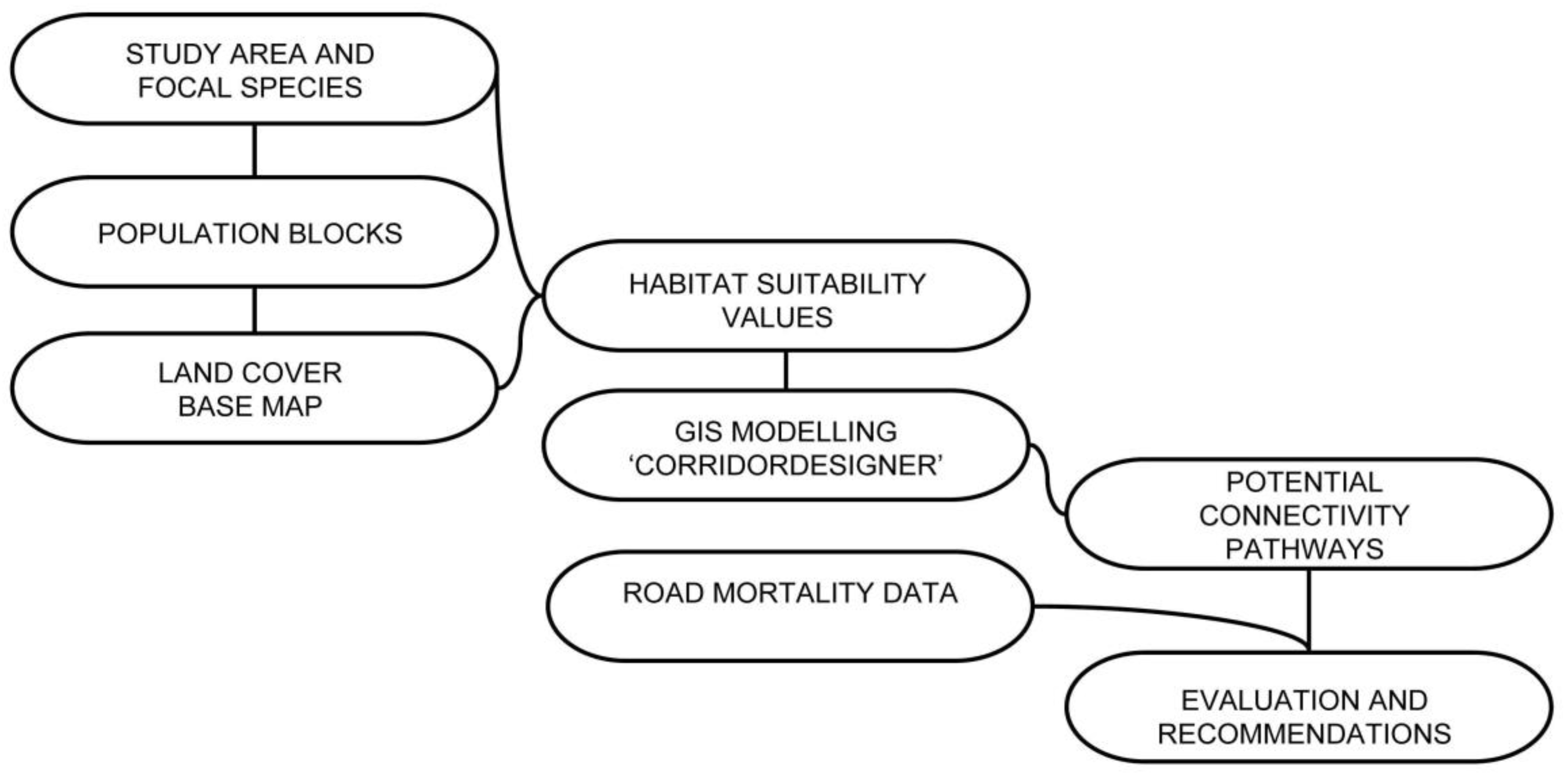
2. Materials and Methods

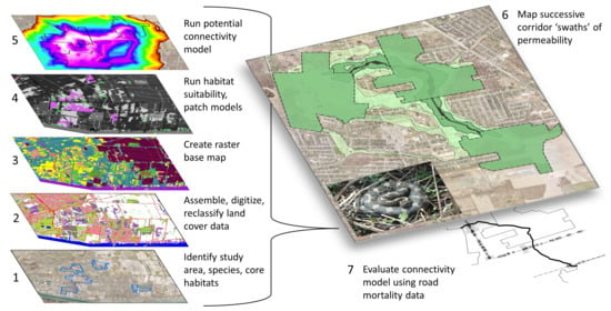
After defining the focal species and study area, five large habitat ‘blocks’ were chosen between which to model potential connectivity. A land cover base map depicting multiple land cover classes was then created with readily available GIS data layers. Next, habitat suitability values were assigned to each land cover class following a literature review of habitat and dispersal characteristics of the focal species. Finally, a cost-surface modeling tool, CorridorDesigner [28], was used to model potential connectivity pathways (PCP) in ArcGIS. PCPs were then subject to an evaluation using guild-based road mortality data (Figure 1).

2.1. Study Area

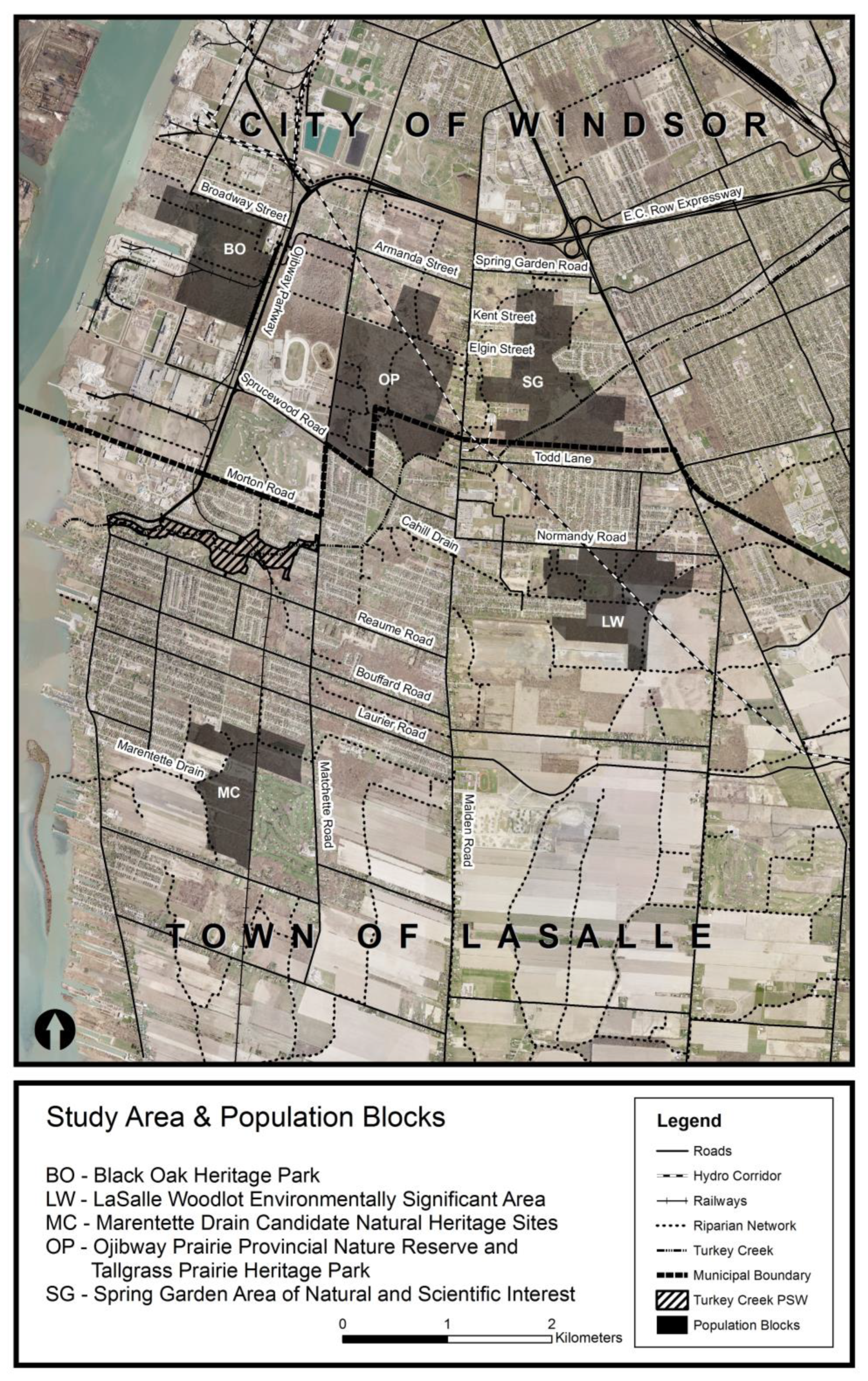
The study area is an 80 km² region within the urban/urbanizing landscape of the City of Windsor and Town of LaSalle, and was chosen to include all known Massasauga observations dating back to the 1980s (Figure 2) [14]. An extensive set of land uses are present in the study area, including residential, industrial, recreation, agricultural, multi-use parkland and nature reserve parkland. The study area includes the entire Ojibway Prairie Complex (OPC) and nearby natural areas (i.e., OPCGPE), in addition to other Town of LaSalle candidate natural heritage (CNH) sites. Protected area and CNH site boundaries were estimated through official plan documentation, grey literature and Ecological Land Classification data from the Essex Region Conservation Authority. The study area is experiencing rapid land-use change due to recent and ongoing developments within the City of Windsor (residential development, provincial highway expansion, new international bridge crossing, and ‘big box’ commercial development) and the Town of LaSalle (community expansion into agricultural land).

We identified five ‘population blocks’ within the study area using the following criteria: size, presence of suitable habitat, absence of through roads, protected status, and current or historic species occurrence (Table 1). At least four of five criteria were met by each of the five blocks: (1) Black Oak Heritage Park (BO), (2) Ojibway Prairie Provincial Nature Reserve and Tallgrass Prairie Heritage Park (hereafter ‘Ojibway Prairie’; OP), (3) Spring Garden Area of Natural and Scientific Interest (hereafter ‘Spring Garden’; SG), (4) LaSalle Woodlot Environmentally Significant Area (hereafter ‘LaSalle Woodlot’; LW) and (5) Marentette Drain Candidate Natural Heritage Sites (hereafter ‘Marentette Drain Woodlots’; MC) (Figure 2). Population block boundaries were mapped in a GIS while referring to aerial imagery, official planning documents, parcel data and/or Ecological Land Classification data. Boundaries for four of the blocks (BO, SG, OP, and LW) follow existing protected area boundaries in official planning documents. The boundary for MC was drawn to encompass seven adjacent CNH sites, the narrow bands of agricultural land in between them, and the adjacent rail corridor [29]. The area of each block was calculated in a GIS and sizes ranged from 76 ha (MC) to 140 ha (OP). Potential connectivity pathways were modeled between each of the population blocks.

2.2. Land Cover Base Map

A detailed land cover raster map was created for the study area (using a cell size of 15 m) and was used as the base map for all modeling. Land cover data were acquired through the University of Guelph Data Resource Centre and were uploaded into a GIS using ArcMap 9.2. The base map was compiled from four separate datasets: (1) ecologically based land cover, (2) riparian network, (3) railway rights-of-way, and (4) road network. A total of 19 land cover classes were represented which generally follow Ecological Land Classification (ELC) definitions (seven classes are non-ELC). Raster codes for each land cover class followed those used in the ‘Ecologically based land cover’ dataset, with additional codes assigned as needed. Each dataset is described in detail below.

Ecologically-based land cover data were acquired through the Southern Ontario Land Resource Information System (SOLRIS, 15 m cell size) [36], which included vegetation communities, hydrology (open water), urban features (pervious, impervious, extraction), roads and an ’undifferentiated’ category of land cover. The three golf courses within the study area were originally classified as either ‘extraction’ or ‘urban pervious’. These were selected and reclassified into a separate land cover class, ‘golf course’ with a new raster code. The ‘undifferentiated’ category encompassed a large proportion of the study area, and combined a variety of land cover types that might influence dispersal of the focal species in different ways, and therefore it was subdivided and re-categorized using aerial imagery from the Southwestern Ontario Orthophotography Project (SWOOP, 30 cm resolution) [37]. For example, agricultural lands and forest clearings were combined in this category, however, the former is likely much less permeable to dispersal of focal species than the latter (Table A1). The original SOLRIS layer was converted into vector format and all polygons originally classified as ‘undifferentiated’ were selected and saved as a new layer. Polygons within this layer were reclassified into one of five categories: (1) open water, (2) urban impervious, (3) urban pervious (4) agricultural lands, and (5) naturalized open area. The first three categories already existed in the SOLRIS database whereas the last two were new categories.

Reclassification of SOLRIS data was done by overlaying the polygons on aerial imagery at a 1:10,000 scale. In general, the land use type that appeared dominant within each polygon was the one assigned. Active agricultural lands were identified from their uniformity of colour (light tan, dull green) and texture. Residential areas, concentrations of buildings, or roads were identified by their characteristic structure and classified as ‘urban impervious’. Some new residential developments not previously identified by SOLRIS were digitized during this step. Large portions of backyards or lawn (bright green) were categorized as ‘urban pervious’. All other areas which appeared to be dominated by open vegetation communities (savannah, meadow or naturalized farm land; irregular in texture and brownish vegetation) were categorized as ‘naturalized open area’. Some polygons were cut into two or more separate polygons to reflect differences in land use types within the original polygon. All reclassified polygons were then converted back to raster form and mosaicked overtop of the original SOLRIS layer. Many polygons were difficult to accurately differentiate and the reclassification was rough at best. Despite this, the procedure provided a greater level of land cover detail than what existed in the original ‘undifferentiated’ category.

The riparian network dataset was created to represent smaller linear water features that were otherwise excluded from the SOLRIS dataset (due to the 15 m resolution), and was intended to represent the topography and riparian vegetation associated with linear water features, as well as the water features themselves. First, the riparian network layer [38] was edited using aerial imagery (SWOOP) to remove all linear water features that corresponded to waterways ≥15 m (majority of these features were already categorized as ‘Open Water’ in the SOLRIS dataset). As a result, the layer was edited to represent smaller surface water features such as large open swales, small creeks and agricultural drains (but not small roadside swales). Next, linear water features which appeared to intersect features in the ‘urban impervious’ category of the SOLRIS layer were either removed or cut at appropriate locations so that they would not overlap the latter category. The resulting polyline riparian network was converted to raster (15 m cell size).

The railway rights-of-way dataset was created to fully represent these linear open features, which were not always apparent in the SOLRIS dataset. First, railway rights-of-way [39] were buffered to 30 m or 15 m (main line and sidetracks, respectively) based on different right-of-way (ROW) widths measured in a GIS (using SWOOP imagery). For example, a sidetrack through a forested area to an industrial facility had a ROW width of ~15 m, whereas a main line between a forest and a residential area was ~30 m wide. Sidetracks were limited to the industrial areas of the study site whereas the sole main line passed through both industrial and residential areas and ran the entire length on the study site (North to South). The railway rights-of-way layer was converted to raster format with a 15 m cell size.

The road network dataset was created using the original ‘transportation’ layer from SOLRIS [36]. This layer was extracted and recategorized to reflect the variation in traffic level between different road categories. Roads were categorized into four main groups based on road width and classification in official plans [22,40], and classification was assumed to be an indicator of traffic volume. All roads with a minimum of four lanes and classified as either ‘provincial highway’, ‘arterial road’ or ‘controlled access highway’ in official plans were compiled into a separate layer and classified as ‘four-lane highways and arterials’. All two-lane roads classified as either ‘collector road’ or ‘arterial road’ were compiled into a separate layer and classified as ‘two-lane arterials and collectors’ (Two roads not labeled as collector or arterial were included in this category due to their temporary function as such due to an adjacent collector/arterial road under construction). All other roads were identified as ‘local roads’ (e.g., gravel, paved roads, private laneways, and incomplete collector/arterial roads). Designated bicycle trails were included in a separate layer, ‘trails’, by referring to the City of Windsor ‘bikeways’ as well as the Town of LaSalle ‘asphalt recreation way’.

2.3. GIS Modelling

GIS modeling followed methods outlined by Beier et al. [6] for designing wildlife corridors between ‘wildland blocks’ using the ArcGIS toolbox extension ‘CorridorDesigner’ [28]. The CorridorDesigner tool was used to model potential connectivity pathways (PCPs) between population blocks. This was done by first creating an overall habitat suitability model (HSM) based on suitability values and then modeling suitable habitat patches. For each set of population blocks, a cumulative cost map (CCM) was created from the HSM, depicting landscape permeability between selected blocks. A series of successive rank-ordered swaths of permeability were produced from the CCM.

2.3.1. Habitat Suitability Model

The habitat suitability model (HSM) tool in the CorridorDesigner toolbox was used to create the habitat suitability model. The tool was used to reclassify all raster cells of the land cover base map into their associated suitability values. Each land cover class was assigned a score to reflect its relative habitat suitability for the focal species (Table A1). Land cover classes were scored from 0–100 following the method applied by Beier et al. (strongly avoided [0–39], occasionally used for nonbreeding activities [40–59], useable for breeding but suboptimal habitat [60–79], and, best habitat for breeding and survival [80–100]) [6]. Classes were scored in units of 10 while single units were used to differentiate between classes with similar suitability but slightly different permeabilities. For example, all roads are unsuitable habitat, however roads with higher traffic volumes (e.g., four-lane highways and arterials) are presumed to be less permeable to snake dispersal than roads with lower traffic volumes (e.g., local roads) [41,42]. Suitability values were then used to create a simple American Standard Code for Information Interchange (ASCII) table for input into the CorridorDesigner tool. This table was of the following format: ‘in_value: out_value’, where the original raster code for a particular land cover type was the ‘in_value’ and the associated suitability score was the ‘out_value’.

The land cover base map and ASCII table were used as inputs in the HSM tool. Although the tool allowed for the input of other factors that might influence habitat suitability (e.g., topography, distance from roads), land cover was chosen as the sole factor influencing habitat suitability for the focal species in the study landscape. The output habitat suitability model was a new version of the original land cover base map wherein the original raster codes were reclassified on a scale of 0–100 to reflect the relative suitability of land cover classes within the study site.

2.3.2. Habitat Patch Model

The habitat patch model (HPM) tool in the CorridorDesigner toolbox was used to model potential breeding patches, defined as patches of habitat capable of supporting a single breeding event based on suitability and size, within population blocks. These patches functioned as start and end points for the connectivity modeling step. The HPM was created from the input HSM. The suitability threshold was set to 61, to exclude forested areas (suitability value = 60). Although forest/swamp areas can be found within a home range (i.e., used as overwintering areas), forest pixels were excluded from the suitability threshold to avoid the model producing suitable habitat patches of large expanses of forested areas with little to no open habitat. For certain land cover classes, suitability values were assigned with the HPM in mind: these classes were given a score based on how suitable a pixel of that particular class would be when immersed within or adjacent to an otherwise suitable habitat patch. As a result, the HPM map produced more realistic patches that were not bisected by relatively permeable features (e.g., hedgerows, riparian, trails, etc.). The perceptual range of the focal species was assumed to be small and therefore the moving window was selected to be a circle of 15 m (i.e., one pixel). The moving window assessed the suitability of each pixel based on the average suitability of only those neighboring pixels in direct contact with it [43]. The use of a circle as opposed to a rectangle ensured that roads were not included within a suitable habitat patch. The breeding patch threshold was set to 5 ha. This was assumed to be the smallest patch size necessary to support a single breeding event [6] and was based on the size of an open habitat patch in the study area that consistently produced Massasauga records over a 10-year period from 2000–2010. The patch size is also presumed to be large enough to support the overlapping home ranges of a male and nongravid female Massasauga, based on a nearby population in Michigan (3–7 ha) [44].

2.3.3. Potential Connectivity Model

The corridor model (CM) tool in the CorridorDesigner toolbox was used to model potential connectivity pathways (PCP). We defined a PCP as a continuous zone of varying width which links population blocks. We used pixel swaths as opposed to single pixel-wide least-cost paths to model potential connectivity, because pixel-wide paths are highly sensitive to cell classification errors and are undesirable for guiding intervention locations due to their narrow width [6]. Furthermore, a single least-cost path lacks any measure of certainty, and equal or very similar cost values could be obtained by totally different, yet unmapped, pathways [45].

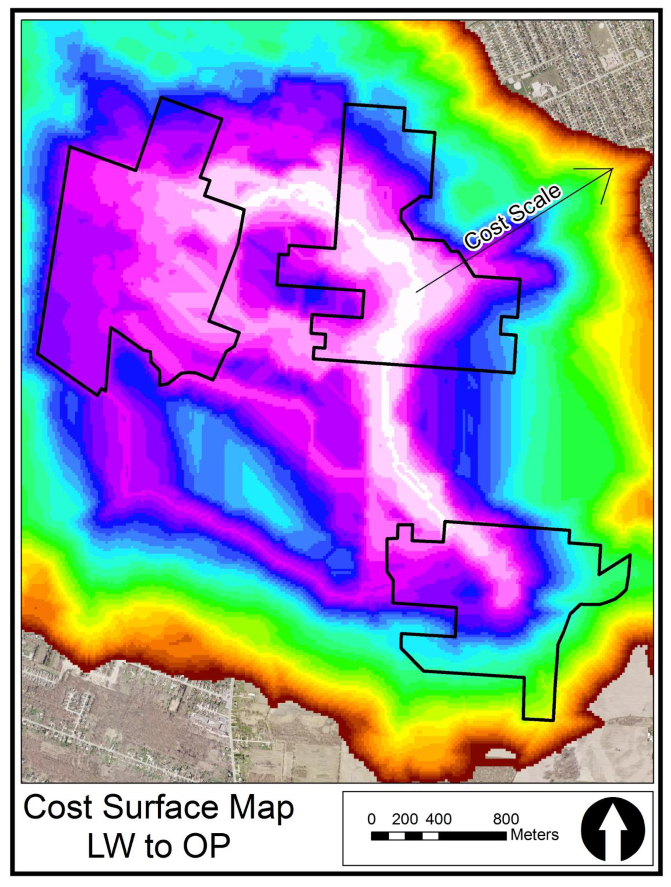
The CM tool applies cost-weighted distance analyses, a form of least-cost modeling to identify the swaths of lowest relative resistance between population blocks (resistance is assumed to be the inverse of suitability). The tool was run between seven different sets of population blocks, but for each model run only two blocks were chosen. For each block a potential breeding patch (from the HPM) was used as the PCP terminus (the largest or most centrally located breeding patch in a block). Potential breeding patches and the HSM were used as model inputs. The moving window used was the same size and shape as the one used for the HPM. Two ‘behind the scenes’ analyses are conducted by the CM tool: a habitat suitability averaging map (HSAM) and a cumulative cost map (CCM; Figure 3). The HSAM is an averaging out of the HSM based on the moving window value, and the CCM is calculated from the HSAM. The CCM is based on a calculation of the cost-distance of each pixel, which is the lowest possible cumulative resistance from that pixel to both terminuses. The CCM depicts gradated landscape permeability between terminuses of selected population blocks.

A series of 11 nested ‘permeability swath’ polygons were produced from the CCM which depict successive swaths of permeability (0.1%, 1%, 2%...10%). For example, the 0.1% swath depicted the most permeable 0.1% of the landscape area between population blocks. Each swath is defined by the largest cost allowed within that particular polygon. As each successive swath was activated, the most permeable pathway (0.1%) is widened and new pathways appeared. High-ranking PCPs were selected based upon the most permeable 0.1% and 1.0% of the landscape between each pair of population blocks. Lower ranking PCPs were identified by activating successive permeability swaths and identifying new ‘loops’ between population blocks. Successive swaths were activated until no new PCPs were identified or until the 6.0% permeability swath was activated (generally beyond that level, swaths became too wide to provide any meaningful insight).

2.4. Road Mortality Data

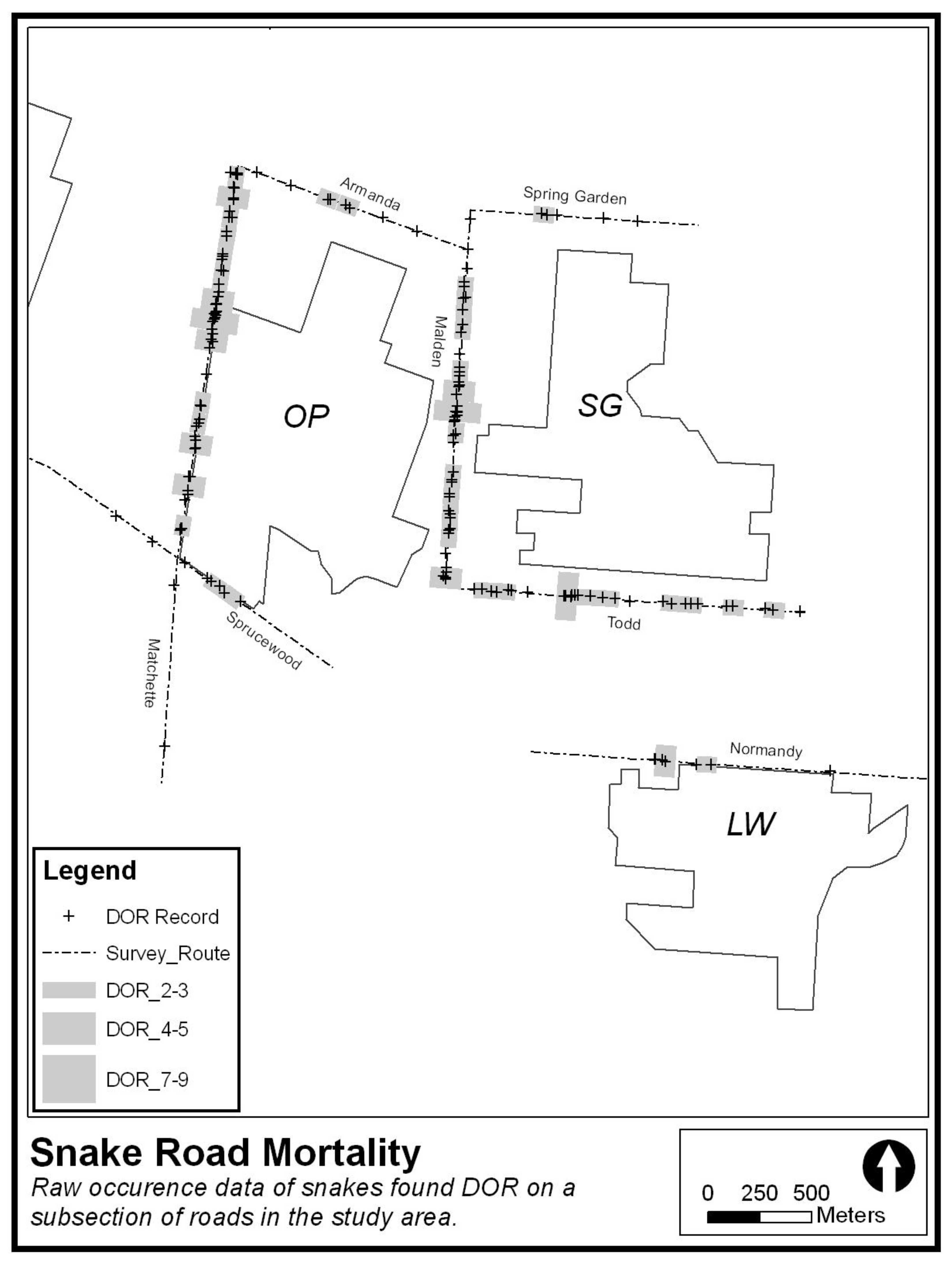
Snake road mortality hotspots were used to evaluate locations where high and low-ranking PCPs intersected with roadways. Hotspots were identified as one or more adjoining road segments (100 m) with relatively high amounts of snake mortality records. Road mortality records were compiled for six snake species (Table 2), spanning five years (2005–2010) and included only ‘dead on road’ (DOR) records with specific location data. Records were derived from (1) data collected during a systematic road mortality study conducted on seven roads in the study area (n = 137; May–August 2010), and (2) a collection of incidental snake road mortality records collected from a variety of local sources (n = 45; 2005–2010) (see Choquette and Valliant [46] for incidental and systematic data collection methods). All records are limited to the seven roads surveyed systematically in 2010 (Figure 4). Snake road mortality data were uploaded into ArcGIS 9.2 and overlaid on SWOOP aerial imagery. Study roads were divided into segments of equal length (100 m), in such a way as to capture the highest number of snake DOR in the shortest distance possible. The total number of snakes and number of species were recorded for each road segment. Segments were categorized based on the frequency of DOR per 100 m: 2–3, 4–5, 6–9.

We were unable to include any Massasauga DOR records in the road mortality dataset (Table 2), due to an absence of data. For example, our four-month road mortality survey conducted in the study area in 2010 found 137 dead snakes but failed to encounter any Massasaugas DOR (additional systematic sampling also failed to detect any [46]). Massasaugas are known to cross roads and become killed on roads [30,33], however in our study area it is likely that few or no individuals were being killed on roads due to small population size; a detailed Massasauga mark-recapture study from 2013–2018 estimated an average of only 10 individuals (juveniles and adults, excluding neonates) remaining in each year (JDC unpub. data). Therefore, road mortality records for the other five snake species in the area (Table 2) were combined and were used as proxies for where Massasaugas were most likely to be killed on roads.

Although Massasaugas have different ecology and behavior than other snake species in study area, there is good reason to use snake road kill hotspots as indicators of Massasauga crossing locations for several reasons. Multiple studies have found spatial clustering (or higher frequency) of road mortality in snakes [41,48,49,50]. These clusters are most common where roads bisect suitable habitat or specific habitat features [33,41,48,49,50,51,52,53,54,55]. Second, spatial locations of high road mortality frequency appear to overlap across species of snakes that utilize similar habitats [56]. Third, all six snake species in or near the study area utilize similar open, early successional habitats such as prairies, meadows, old fields, marshes or forest edges (JDC unpub. data) [31,57,58,59]. Finally, the study area is urban/suburban in nature with a mix of industrial, commercial, residential and natural areas, where natural habitat patches are fragmented and limiting. It is therefore logical to expect clustering of snake road kill where roads bisect ideal snake habitat and to expect multiple or most species (including Massasaugas) to be represented within those clusters.

Although relatively high levels of road mortality have been associated with curves in roads [54], roads in our study landscape are all straight, so this is unlikely to have an influence on the observed road mortality locations. The roads surveyed in this study were also all collector or arterial class roads which function mostly as throughways; therefore, traffic intensity is probably uniform along their lengths. Further, although most of the records we used were from a single season, Langen et al. [55] found that one survey provided a valid snapshot of spatial patterns of herpetofauna road mortality and spatial patterns remained stable across time.

An updated and larger road mortality dataset using only systematic data collected from 2010–2013 (n = 384) [46] was used to calculate the average number of snakes killed per 100 m of road inside and outside of the bounds of the 0.1% and 1.0% permeability swaths. This was done for four PCPs that crossed a subset of the roads (Malden, Matchette, Normandy, Sprucewood and Todd). The average number of snakes killed per 100 m was calculated by dividing the number of road mortality observations by the length of road for each condition (outside the bounds of the PCPs, within the bounds of the 1.0% swath, and within the bounds of the 0.1% swath), and multiplying this value by 100. It should be noted that both observations and road length that fell within the bounds of the 0.1% swaths were included in the calculation of the average number of snakes killed per 100 m for the 1.0% swath. Due to the very small sample size (i.e., number of roads intersected by PCPs and with available road mortality data; n = 5), we were unable to run any meaningful statistical analyses on this variable; however, base data and statistics are presented.

3. Results

3.1. Potential Connectivity Pathways

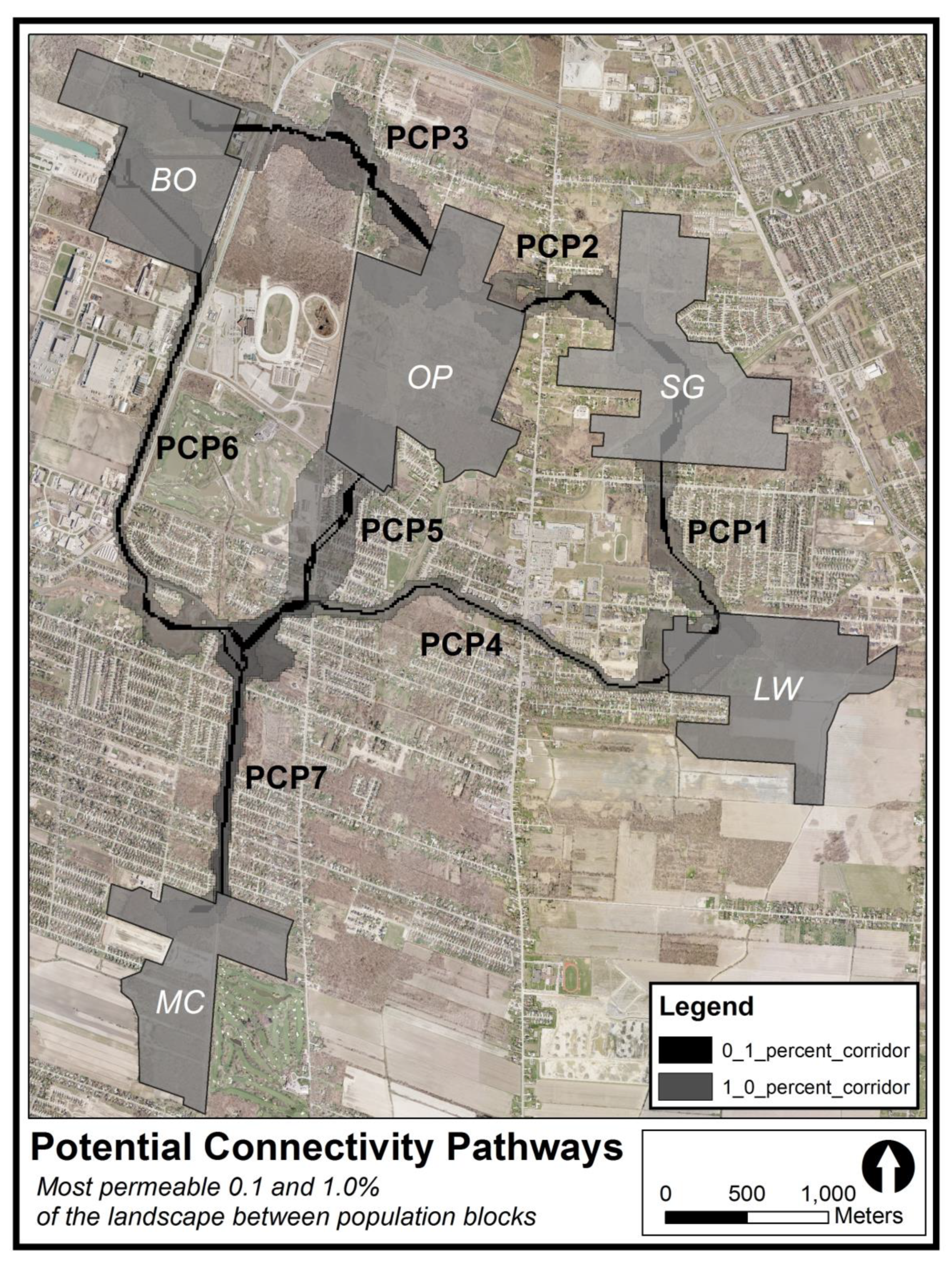
Seven high-ranking potential connectivity pathways (PCP1 through PCP7) for Massasaugas were identified between population blocks (Figure 5). All blocks were linked by one to three pathways. Three separate PCPs (4 through 6) intersected at the Turkey Creek Provincially Significant Wetland (PSW) to become PCP7. Due to its central location, the Ojibway Prairie (OP) population block was linked to other blocks via the highest number of PCPs (n = 3). As the permeability threshold for each PCP increased (>1.0%), high-ranking pathways widened and developed additional strands; these were best viewed and interpreted at a finer scale.

3.1.1. LaSalle Woodlot to Spring Garden (LW to SG)

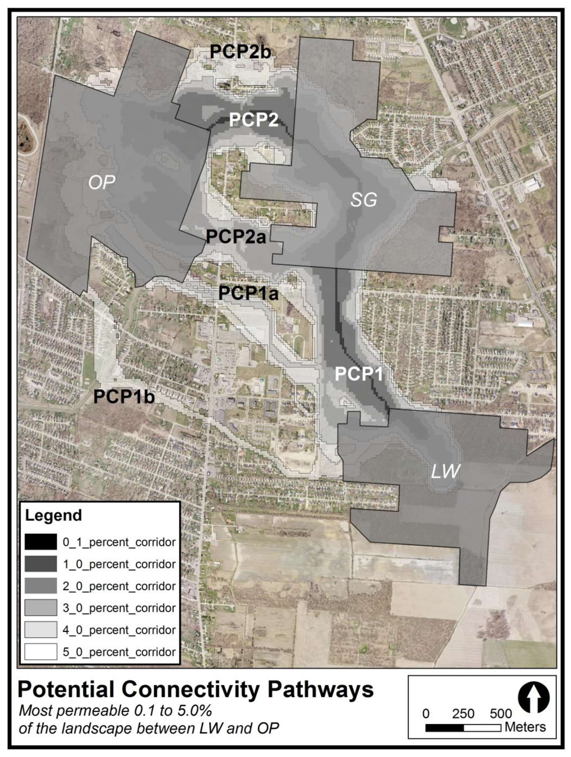
PCP1 was the sole pathway modeled between LW and SG (Figure 6). At the 0.1% threshold, it crosses Normandy Road into a small private woodlot, runs along a hydro corridor, and then cuts up through an undeveloped natural area and across a single row of houses. It then crosses Todd Lane, cuts through another single row of houses before linking up with SG. At the 1.0% threshold the pathway widened to include the entire width of the hydro corridor, part of an undeveloped natural area and encroached upon the first row of residential lots backing onto the hydro corridor and the natural area. The width of the 1.0% pathway across Normandy Road is ~140–250 m and ~200–210 m across Todd Lane. At the 2.0% threshold, the pathway widens to include a 100 m strip of residential land on its East side and includes an additional loop across Normandy Road to the West of the main pathway. Beyond this threshold the pathway continues to widen until the entire landscape in between the blocks is included.

3.1.2. Spring Garden to Ojibway Prairie (SG to OP)

PCP2 is the highest-ranking pathway between these two blocks (Figure 6). The 0.1% pathway widens (~150 m) as it passes through a patch of meadow habitat and then narrows (~60 m) as it passes through a large residential lot. It then crosses Malden Road at a location bordered by residential properties, and then cuts through two of these properties and an open field before linking to OP. The 1.0% pathway is much wider than the 0.1% pathway (at Malden Road: ~320 m vs. ~50 m, respectively), and includes a wide zone of land between both blocks with large-lot (12) and small-lot (9) residential dwellings. PCP2b is identified by the 2.0% swath. It is a wide loop running north that passes through a large meadow patch with small residential lots (6), crosses Malden Road (width ~150 m), and through large residential lots (4) before continuing through a large area of forest and meadow before connecting to OP. The 3.0% swath identifies an additional PCP (2a) that links the southern portion of SG to OP, and crosses Malden Road near a hydro corridor at a width of 90 m. At the 4.0% swath, almost the entire landscape between OP and SG is included.

3.1.3. LaSalle Woodlot to Ojibway Prairie (LW to OP)

This model identifies two main alternatives for potential connectivity between these population blocks: indirect via the SG block, and direct. The first alternative is identified by the most permeable swaths (0.1, 1.0, 2.0 and 4.0%) while the second is identified by less permeable swaths (3.0, 4.0 and 5.0%). Only corridor swaths up the 5% level produced additional PCPs (Figure 6). The indirect alternative follows PCP1 from LW to SG and then follows three possible PCPs from SG to OP. From most to least permeable these are: PCP2 (0.1 & 1.0% swaths), PCP2a (2.0% swath) and PCP2b (4.0% swath). PCP1 and PCP2 combined represent the most permeable route between both population blocks, while PCP1 and PCP2a combined represent the second most permeable route. The direct alternative identifies two PCPs between LW and OP. PCP1a is identified by the 3.0% swath, and is essentially a side loop off of PCP1 that follows an open swale to the west and finally continues along a large creek into OP. PCP1b is identified by the 5.0% corridor and follows a municipal drain to a large creek, where it runs northwest through a residential area and across Sprucewood Road into OP.

Four of the PCPs modelled between LW and OP were also identified by the LW to SG and SG to OP models but are slightly different. The SG to OP model identified PCP2 as being much wider at the 1.0% swath than the LW to OP model (300 m vs. 200 m at Malden Road). Also, PCP2b was identified in the SG to OP model at the 2.0% swath, whereas the LW to OP model identified it at the 4.0% swath (almost identical locations). PCP2a was identified in the SG to OP model at the 3.0% swath, whereas the LW to OP model identified it at the 2.0% swath (again, at the almost identical location). For PCP1, the 0.1% and 1.0% swaths are almost identical between models.

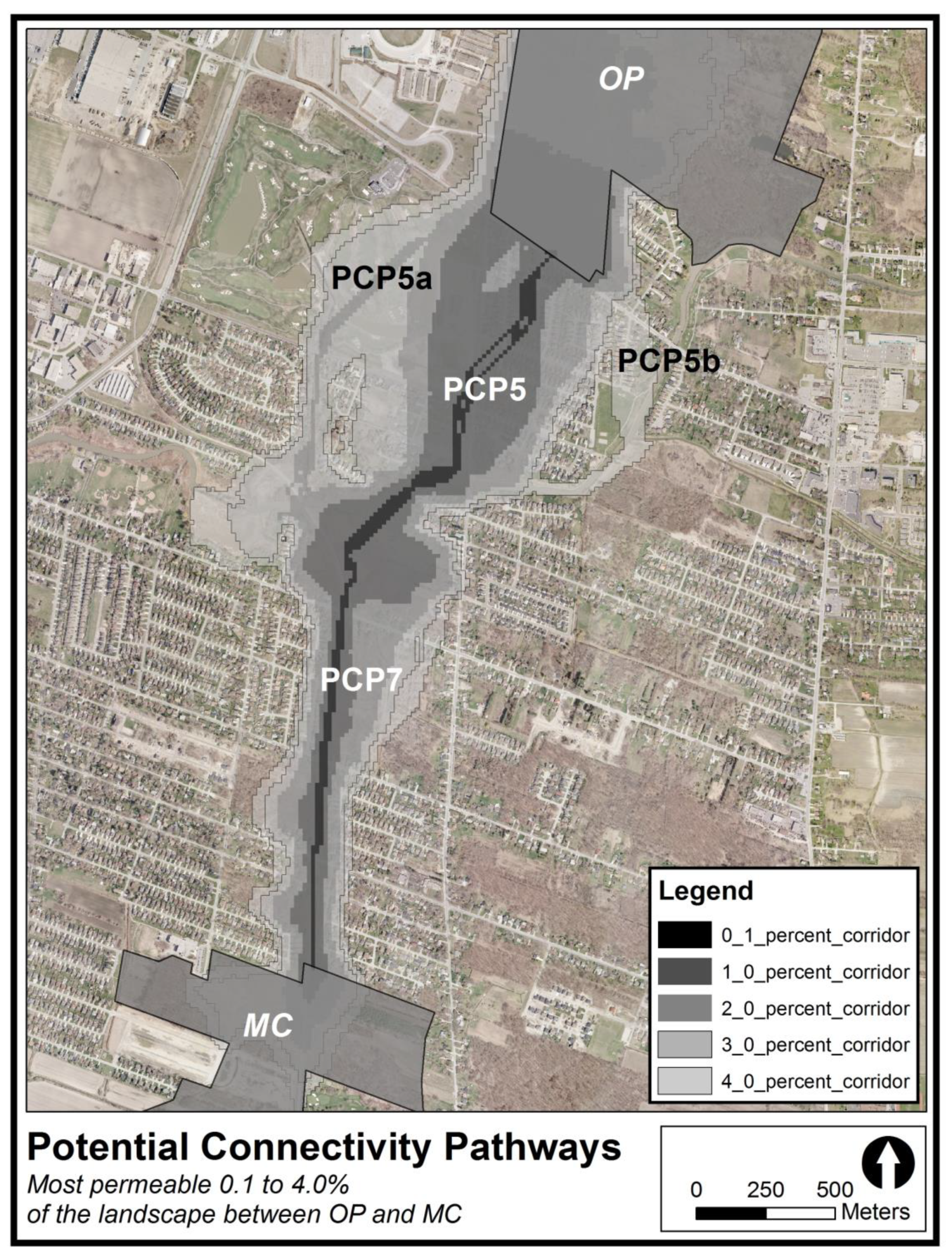
3.1.4. Ojibway Prairie to Marentette Drain Woodlots (OP to MC)

These population blocks are linked by PCP5 and PCP7 (Figure 7). The 0.1% pathway exits OP midway along its southern boundary, crosses Sprucewood Road and cuts through a residential subdivision. It then crosses two perpendicular roads northwest of their intersection before crossing south through a relatively low-density residential area and then into the Turkey Creek PSW. The linkage continues south as PCP7, following a rail corridor and crossing three roads before connecting to MC. At the 1.0% swath, PCP5 widens to include the southern boundary of OP, a large section of road, and portions of a golf course (~150 m band) and residential subdivision (~200 m band). The pathway widens at the Turkey Creek PSW before continuing south along PCP7 where it widens to between 75–125 m, and includes residential properties and natural areas adjacent the rail corridor. Between the 1.0% and 4.0% swaths the model identifies additional PCPs linking OP and MC (PCP5a, PCP5b). No additional loops are identified along PCP7.

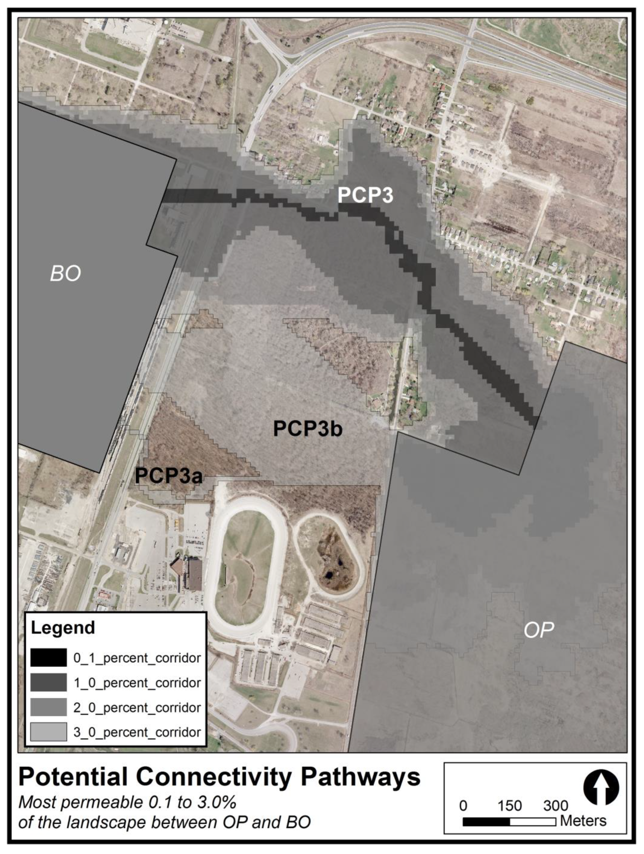
3.1.5. Black Oak Heritage Park to Ojibway Prairie (BO to OP)

These two blocks are linked by PCP3 (Figure 8). The 0.1% pathway follows a hydro corridor from the north end of OP, cuts through a large residential lot, passes through a meadow and then crosses Matchette Road. It cuts across the north end of Ojibway Park (a distinct park from OP), crosses a road and a field, before crossing the same road again and continuing west through Ojibway Park. The pathway then crosses the four-lane Ojibway Parkway, a rail corridor and then an industrial facility before linking to BO. The 1.0% swath widens substantially along the hydro corridor (~200–250 m), includes a wide band along the north end of Ojibway Park (~125–250 m), a patch of open field and a wide swath between the western boundary of OP and BO (~400–425 m). In addition to PCP3, two additional pathways are identified; PCP3b (3.0% swath) passes between OP and BO through the middle of the forested Ojibway Park, and PCP 3a is a small side loop branching south off of PCP3b.

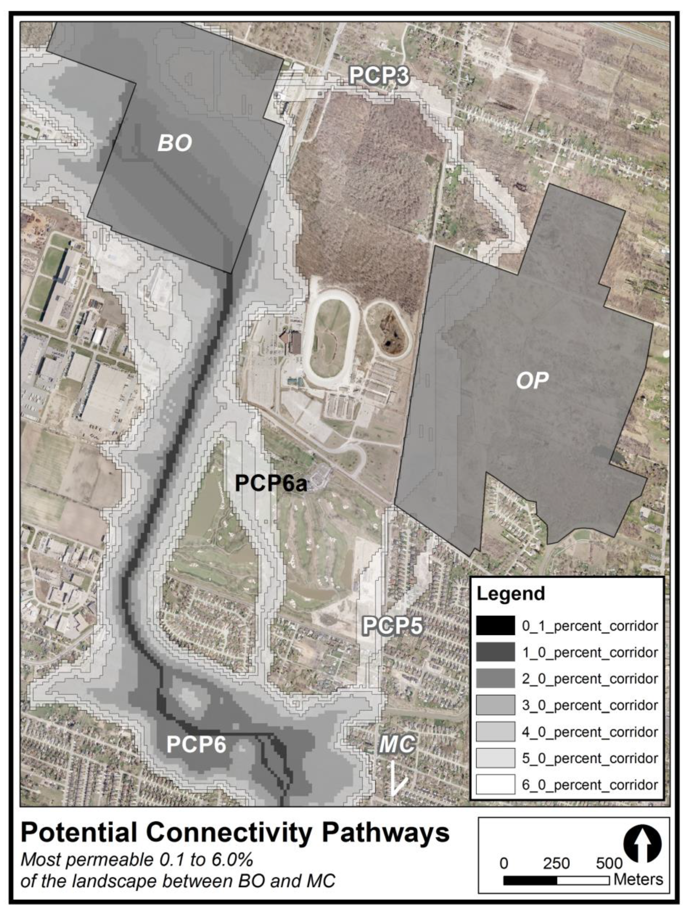
3.1.6. Black Oak Heritage Park to Marentette Drain Woodlots (BO to MC)

The model presents two alternatives for potential connectivity between blocks: direct, and indirect via OP (Figure 9). Both alternatives pass through the Turkey Creek PSW (Figure 9). The direct alternative includes PCP6 and PCP7 and is represented by the most permeable swaths (0.1–4.0% swaths). The indirect route includes PCP3 and PCP5 and is less permeable (5.0% swath). The 0.1% swath exits BO at the southwest corner and continues south along a rail corridor, crosses a highway, continues along the rail corridor and cuts across a residential area before entering the Turkey Creek PSW. It then continues west through the wetland area, producing a double loop around a section of rail corridor and then continues south to MC as PCP7 (see Section 3.1.4). The 1.0% pathway becomes slightly wider along PCP6 (~30–45 m) as it follows the rail corridor and develops two loops as it enters the wetland area, the first follows the 0.1% pathway (although much wider: ~175 m). An additional pathway is identified by the 4.0% swath (PCP6a) which crosses through industrial land, a highway, a golf course, and a riparian corridor, before entering the Turkey Creek PSW. The indirect route between BO and MC is not identified until the 5.0% swath and follows PCP3 to OP and then to MC via PCP5 and PCP7 (Figure 7 and Figure 8). In this case, PCP5 is represented by two loops: one running through a golf course (5.0% swath) and the other through a residential area (6.0% swath).

3.1.7. LaSalle Woodlot to Marentette Drain Woodlots (LW to MC)

The model presents one main possibility for potential connectivity between these blocks (Figure 5). The 0.1% pathway follows PCP4 toward the Turkey Creek PSW along a municipal drain and then follows PCP7 south along a rail corridor to MC. The 1.0% pathway includes a trail network adjacent to the municipal drain and encroaches 20–30 m onto residential and commercial land uses. The PCP widens to 100–150 m when it runs along a candidate natural heritage site at the confluence of the municipal drain and a creek, and also widens within the wetland area itself. The pathway between LW and MC continues to widen in small increments beyond the 1.0% swath. The 7.0–10.0% swaths reveal a web of looping strands running southwest from LW between the population blocks (not mapped).

3.2. Road Mortality Analysis

3.2.1. Snake Road Mortality Hotspots

The snake road mortality dataset covered seven arterial and collector roads in the study area (Figure 4). Results are only presented for five study roads that were also intersected by PCPs (Malden, Matchette, Normandy, Sprucewood, and Todd). Road mortality hotspots varied in intensity and length across study roads. On Normandy Road the hotspot was represented by a single segment with four to five DOR records. On Todd Lane there were five distinct clusters of snake road mortality. Each cluster consisted of one to three adjoining road segments with two to nine DOR records each, and were separated from nearby clusters by one or two road segments. The hotspot is represented by a cluster of three adjoining segments, one of which contains seven to nine DOR records. On Malden Road there were also multiple clusters of snake mortality. Four main clusters were identified, each consisting of one to four adjoining road segments with two to nine DOR records each, and separated from nearby clusters by one road segment. One cluster, made up of four road segments, is the only one containing a segment with seven to nine DOR records and stands out as the hotspot (Figure 4). Four snake mortality clusters were also identified on Matchette Road. The hotspot consists of nine adjoining segments with between two and nine DOR records each, and is the longest hotspot in the study landscape. Within the Matchette Road hotspot there are two segments that stand out: the first is a segment containing four to five DOR records at the north end of the hotspot, and the second is a segment containing seven to nine DOR records at the south end of the hotspot. Finally, the hotspot along Sprucewood Road consists of two adjoining segments with two to three DOR records each.

3.2.2. Potential Connectivity Pathways in Relation to Hotspots

Four high-ranking PCPs (1, 2, 3, and 5) intersected roads through or near road segments with relatively high levels of snake road mortality (i.e., hotspots). On roads intersected by the latter four PCPs (Malden, Matchette [north of Sprucewood], Normandy, Sprucewood and Todd) the average number of dead snakes observed per 100 m of road (±SE; n = 5) outside of the boundaries of the 1.0% PCP swaths was 3.09 ± 1.11. Within the boundaries of the 1.0% and 0.1% swaths, the average number of dead snakes per 100 m of road was 6.46 ± 2.27 and 5.30 ± 2.76, respectively (Table 3).

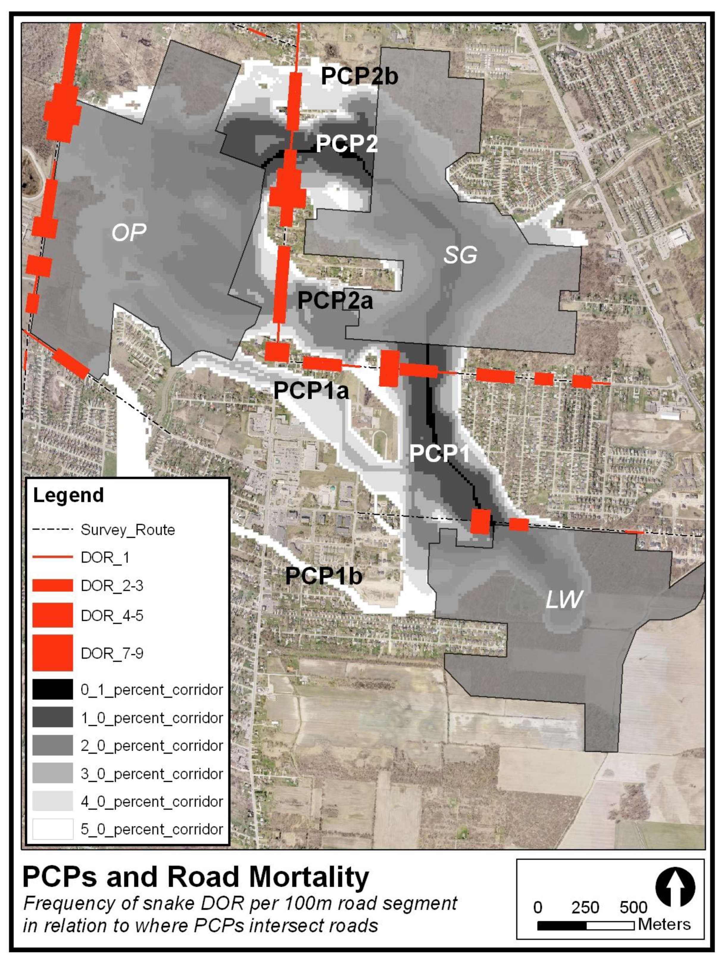
PCP1 intersects Normandy Road directly adjacent to the road mortality hotspot (~60 m from centre of hotspot to centre of PCP; 0.1% swath), and intersects Todd Lane through the east end of the hotspot on that road (~200 m from centre of PCP to centre of segment with highest mortality rate; 0.1% swath). The Normandy Road hotspot is entirely within PCP1 at the 1.0% swath, whereas the Todd Lane hotspot is not entirely within PCP1 until the 3.0% swath (5.0% swath for the LW to OP model; Figure 10).

PCP2 intersects Malden Road through the north end of the hotspot (~230 m from centre of PCP to centre of road segment with highest mortality rate; 0.1% swath). The majority of the hotspot is included in the PCP at the 2.0% swath (5.0% swath for the LW to OP model; Figure 10). PCP2b intersects Malden Road through the road mortality cluster to the north of the hotspot (2.0% swath; 4.0% swath for the LW to OP model). PCP2a intersects Malden Road through the southern half of the road mortality cluster south of the hotspot (3.0% swath; 2.0% swath for the LW to OP model).

PCP3 intersects Matchette Road at the north end of the hotspot, at a segment with relatively higher mortality records than adjoining segments (and ~620 m from centre of PCP to centre of road segment with highest mortality rate; 0.1% swath). PCP3b intersects Matchette Road at the south end of the hotspot through the segment with the highest frequency of road mortality (3% swath; Figure 11). PCP5 intersects Sprucewood Road in the centre of the road mortality hotspot (0.1% swath), then continues south and intersects Matchette Road at a segment with no snake DOR records. PCP5b intersects Sprucewood Road at a segment with no snake roadkill.

4. Discussion

4.1. Potential Connectivity Pathways

PCPs depict the most permeable portions of the landscape between population blocks for the focal species, and indicate where successful dispersal (i.e., movement leading to spatial gene flow [60]) between blocks would be most likely. Depending on the vagility of the focal species and the length or suitability of the PCP, functional connectivity between blocks may occur directly via seasonal migrations, mate-searching movements, or dispersal of young snakes. Connectivity might also occur indirectly via gradual dispersal of young snakes over multiple generations within the PCP itself. It is important to note that the zone included within a PCP is not necessarily permeable enough to allow successful snake movement between population blocks. Instead, the PCPs identify the most suitable areas to target for interventions aimed at maintaining, increasing or restoring connectivity between blocks (i.e., to direct conservation resources where permeability is already at its highest). Due to the ongoing decline and low abundance of the Ojibway Prairie population of Massasaugas, conservation interventions within PCPs are unlikely to benefit the population in the short term and ought to be conducted within the context of a broader population augmentation or reintroduction initiative.

The model was used to identify two high order PCPs (1 and 2) and three lower-order PCPs (1a, 1b, 2a, 2b) linking three population blocks identified as Critical Habitat for the Massasauga (LW, SG and OP) [24]. Massasaugas are capable of moving a few hundred meters to over one kilometer between hibernation and foraging sites or to seek out mates, however, maximum range lengths vary substantially between populations [14,61,62]. Durbian et al. [30] recommend providing suitable habitat within ~400 m of hibernation sites, and the maximum movement recorded for adult Massasaugas at Ojibway Prairie was just under 700 m (JDC unpub. data). Further, mean range length of neonate Massasaugas is ~60 m [30], with a maximum of ~180 m [63]. The PCPs identified in this study are likely too long (860 m to 2420 m, based on nearest potential breeding patches) to facilitate dispersal of adults or juveniles between population blocks. Functional connectivity will likely depend on the maintenance of suitable breeding opportunities outside of population blocks and subsequent intergenerational dispersal between blocks. As a result, distance between potential breeding patches within the PCPs themselves is an important consideration.

Based on a patch configuration analysis (wherein interpatch distance was compared to a 400 m threshold), four PCPs (1, 2, 2a and 2b) have the greatest potential to contribute to connectivity between Massasauga Critical Habitat and should be the focus of connectivity-based interventions. Connectivity will be dependent on potential breeding patches outside of population blocks, and interventions should focus on these patches (strategic acquisition, restoration, stewardship agreements, etc.). For LW to SG, PCP1 at the 1.0% swath should be used to guide interventions across Normandy Road, whereas further study is needed at Todd Lane (e.g., bridge over Turkey Creek; see Section 4.3). Interventions for increasing connectivity between OP and SG should focus on PCP2 and PCP2a, due to lowest average permeabilities when combining LW to OP and SG to OP models (but see Section 4.2). Our recommendations could be used to guide interventions aimed at increasing the probability that Massasauga Critical Habitat function as an integrated unit. Although Massasaugas can incorporate high-use areas into yearly activity ranges (e.g., hiking trails [64]; roadside habitats [65]), and will use under-road crossing structures [66], conservation practitioners must explicitly address the potential negative impacts of human disturbance on connectivity (e.g., reduced movement [64], fine-scale genetic isolation [67]) to increase the likelihood of beneficial outcomes.

It is important to note that the model outputs were likely sensitive to the number and nature of land cover classes used. For example, some authors have found cost-surface models to perform better (more likely to predict occurrence data) as the number of land cover classes increased [45] or the accuracy of land cover data is increased [6]. When compared to aerial imagery at the broad scale, PCPs (1.0% swath) generally appear to follow suitable habitat or natural areas (a clear exception is PCP5, discussed later). The general accuracy of PCPs might be attributed to the inclusion of additional land cover classes in the base map (beyond those originally in the SOLRIS dataset) which better reflected the habitat use and dispersal of the focal species in the study area. This idea is supported by Verbeylen et al. [45], who found the best model in their study had twice the number of land cover classes than a simpler model (10 vs. 5, although not significantly different).

In our study, the inclusion of two linear land cover classes (‘riparian’ and ‘rail ROW’) provide a good example for how additional classes likely improved model outcomes in a way that better reflected potential connectivity for our target species. The effects of these two classes appear the most pronounced with PCP4, 6 and 7 (as well as PCP1a, 5a and 6b), which follow riparian and/or rail corridors quite closely. These results seem to reflect landscape permeability for Massasaugas, which have been recorded historically and recently using both types of linear features in this landscape (P. Pratt pers. comm. 2010, T. Preney pers. comm. 2011) [35]. Furthermore, the likelihood of the linear classes biasing model outcomes is low because these land cover classes were assigned scores intermediate between highly suitable habitat (e.g., naturalized open area, marsh) and unsuitable habitat (e.g., urban impervious). Therefore, the linear classes had the greatest influence on model outcomes only when the availability of surrounding suitable habitat was low. For example, PCP7 followed a municipal drain corridor through unsuitable commercial and residential land uses, and PCP6 followed a rail corridor through unsuitable industrial lands, but passed through more suitable habitat (i.e., marsh) when it became available. In the original SOLRIS land cover dataset many of the linear features were either unmapped (riparian) or classified as adjacent land cover types which are unsuitable for Massasaugas (rail ROW). Presumably, the absence of these two new land cover classes would have resulted in alternate, less accurate, outcomes.

Erroneous classification of land cover might have influenced model outputs. When we examined PCPs at a fine scale, we noticed some deficiencies where the most permeable (0.1%) pathways are of questionable suitability; Some PCPs pass through an area of low suitability when an apparently more suitable route appears nearby (PCP1, 2, 3 and 5; based on aerial imagery). Beier et al. [6] suggested that the land cover base map is the most error-ridden component of their cost-surface models. It is likely that our base map is also affected by errors in land cover, especially given the dynamic nature of the landscape. Prairies and meadows were poorly mapped and categorized in SOLRIS at the scale of this study, despite being the most suitable habitat type for the focal species. Portions of this habitat type were initially included in the ‘undifferentiated’ category and later classified by us as ‘naturalized open area’ with a very high suitability score. Upon comparing the land cover map with air photos and ELC data, some patches of meadow habitat were also represented by the ‘urban pervious’ category and had been assigned a relatively low suitability score (Table A1). This may have resulted in model inaccuracies due to the avoidance of some patches of ‘urban pervious’ which were in fact suitable meadow habitats. The opposite instances also occurred, wherein residential properties were classified as ‘naturalized open area’, the most suitable land cover class, as opposed to the must less suitable ‘urban impervious’ or ‘urban pervious’. In these cases, PCPs might have included areas which were no more (or perhaps even less) suitable than their surroundings.

4.2. Road Mortality Data

All road mortality hotspots were located on or very near road segments that intersected with high-ranking PCPs, validating the outputs of the model. Furthermore, the average number of snakes killed per 100 m of road was higher within the bounds of the high-ranking PCPs vs. outside (although the small sample size warrants further study). These results are consistent with a study by Grilo et al. [68] that observed a similar pattern in stone martens. In cases where the road segment with the highest number of DOR records lay outside (but near) the PCPs, such as with PCP1 and PCP2, this was most likely due to the erroneous classification of land cover as previously mentioned. This is further supported by the fact that there do not appear to have been any major land use changes between the time the aerial images were taken (2006) and when the majority of roadkill data were collected (2010). A more striking example is that of PCP5; high levels of road mortality to the West of OP coupled with a nearby patch of naturalized vegetation suggest the most permeable route was in that direction, and then south through the golf course. PCP5 instead passes right through ~450 m of residential subdivision (Figure 12). The patch of naturalized vegetation adjacent to OP was classified as ‘urban pervious’ instead of ‘naturalized open area’, which would have better reflected its permeability.

Another good example of both erroneous and inaccurate land cover is PCP2 (Figure 13). This PCP (0.1% swath) intersected Malden Road at least 200 m north of the road segment with the highest number of mortality records, and it might have crossed much closer (or intersected it) if the land cover data were more accurate. First, the PCP crossed Malden Road where two large residential properties were erroneously classified as ‘naturalized open area’ (they were included as part a large patch of that land cover type directly adjacent to the East). Second, at least one patch of meadow-like habitat exists on the west side of Malden Road, adjacent the road mortality hotspot. This patch is identified as ‘urban pervious’ in the land cover base map and assigned a relatively low suitability score. Had the land cover map been more accurate and included greater thematic resolution, the modeled pathway may have intersected Malden Road through or much closer to the highest mortality road segment.

Our study also demonstrated a case where the use of roadkill hotspots might support a PCP that otherwise appears to be inaccurate (based on aerial imagery). PCP5 was found to pass through an unsuitable land cover (residential), likely due to inaccurate land cover classification. Interestingly, however, the PCP at the 0.1% swath directly intersects the road mortality hotspot on Sprucewood Road. Given the land use data (high suitability prairie habitat to the north and low suitability residential area to the south), it is likely that the road mortality hotspot reflects a road segment with high mortality as opposed to a potential crossing location (i.e., unidirectional dispersal heading south from OP, and no dispersal heading north from the subdivision). Further investigation is warranted to check other hotspots, particularly those that support model outcomes, to identify if they do in fact represent attempted movements from both sides of the road (i.e., mortality hotspots with DOR records in both lanes of the road are better indicators of potential connectivity than hotspots with DOR records in only one lane [69]).

4.3. Limitations

Although we attempted to rigorously model potential connectivity pathways for Massasaugas and evaluate outputs with road mortality data, our study had limitations. First, land cover suitability for the focal species was assumed to be synonymous with land cover permeability. The assumption is that the most suitable habitat for the focal species (active foraging and breeding habitat) is most permeable to dispersal, and the least suitable habitat is least permeable. As a result, resistance (or travel cost) was defined as the inverse of habitat suitability/permeability. This assumption was made in the absence of explicit movement data comparing permeability levels of different land cover classes despite the awareness that the model might ‘ignore’ apparently unsuitable habitat that may be suitable for dispersal/migration [6].

An additional limitation regarding the use of suitability scores is that the model outcomes may be sensitive to changes in their relative values. Verbeylen et al. [45] found results from their connectivity model to show sensitivity to variation in resistance values. In our case, there was a wider range of uncertainty surrounding the most ‘appropriate’ suitability score for some land cover classes compared to others. If the scores we assigned to ‘urban pervious’, for example, were too conservative in some locations, we expect PCPs would have inadvertently shifted away from pixels of that land use. PCP3, which was modeled passing through a forested area, might have otherwise shifted slightly to the north of Broadway Road where there is predominance of ‘urban pervious’ land cover. PCP1, which currently runs north through a forested patch to SG, might run farther to the west through a patch of ‘urban pervious’ and then continue north across Todd Lane (closer to the highest mortality road segment). Some of these changes are reflected when using wider corridor swaths but the tradeoff is that as PCPs become wider, their ability to guide precise intervention locations decreases. One way to overcome the suitability score problem is to create and test multiple ‘resistance sets’ and to produce multiple models to reflect alternatives [45].

The majority of the land cover data we used was based on the SOLRIS land cover dataset. These data included a large portion of the study area which was classified as ‘undifferentiated’ and these areas required additional thematic resolution to better reflect habitat use and dispersal by the focal species. It is unknown if the scale of reclassification (1:10,000) is similar to the scale originally used to map SOLRIS data. It could be that this method resulted in a land cover base map which was not entirely uniform, with the reclassified areas mapped in greater detail than the rest of the study area. If so, the model outcomes might be more accurate in areas that were reclassified as opposed to areas originally classified by SOLRIS. An additional limitation to the land cover data is that it does not reflect the most current land use conditions. Land use changes quickly in urban areas and some of the land cover data used (SOLRIS 2000–2002) had already become somewhat obsolete either due to succession of natural areas or ongoing development. This issue was addressed in part during the quality control phase by digitizing some new developments which we were aware of. Due to the size of the study area, however, it quickly became impractical and it was realized that even the air photos being used for interpretation were already outdated [37]. As a result, some PCPs pass through areas that are indicated as more suitable than actual conditions based on existing development. For example: (1) PCP5 (1.0% swath) passes through a portion of a golf course that is now a residential subdivision, and (2) extra loops were produced across Normandy Road on PCP1 through an area of recent development. Municipalities have extensive collections of up-to-date GIS data, some of which is readily available online or through data-sharing agreements. The use of land cover data from municipal planning departments to supplement more extensive land cover datasets at the outset of the study might have helped to reduce uncertainty posed by data obsolescence.

The assumption we made by including linear classes (riparian and rail ROW) is that the entire length of any particular feature is equally suitable, despite the likely presence of sections which might actually be unsuitable to the focal species (e.g., absence of ideal vegetation structure due to mowing). A good example which weakens this assumption can be discussed with reference to PCP1, and where the hydro corridor intersects a road. Although much of the hydro corridor consists of suitable habitat, it was not mapped by us as a unique linear land cover class and left as classified by SOLRIS [36]. PCP1 followed the corridor only partway, avoided a section that was maintained as mowed lawn (classified as ‘urban pervious’) and looped through a wooded residential property. This loop resulted in PCP1 crossing Normandy Road very close to the road mortality hotspot. Had the corridor been mapped as a single land cover class of continuous suitability, the ‘detour’ would have been overlooked and the PCP would have been farther away from the hotspot on Normandy Road. With riparian and rail ROW classes, the model may have been biased toward following their linear route as opposed to being sensitive to unsuitable habitat along their lengths.

The modeling approach we used displays successive swaths of permeability. The 0.1% swath might be considered analogous to a ‘least-cost pathway’ due to the fact that it was usually quite narrow and a single pixel in width. Least-cost paths are subject to error [45] and the modeling of successive pixel ‘swaths’ might be a desirable method for ‘buffering’ potential error in cell classification and land cover data. Connectivity pathways which remain relatively narrow with each successive swath in comparison to pathways which become relatively wide with each successive swath might indicate increased certainty around the location of the least-cost pathway. Wider successive swaths might indicate less certainty around the least-cost path or areas where the landscape is more permeable to the focal species. For example, PCP2 becomes relatively wider at the 1.0% swath than PCP4, which might reflect the fact that the former passes through a more permeable landscape (i.e., lower density residential, more abundant and dispersed patches of natural vegetative cover, and shorter distance between population blocks) than the latter. Furthermore, the use of successive pixel swaths might be appropriate in instances where the 0.1% swath does not appear accurate but perhaps the 1.0% or 2.0% swath appear to include suitable habitat.

The absence of roadside swales from the base map may have masked results. Swales were not mapped as they are 12–13 m narrower than the pixel size used (15 m). Due to their narrow width and proximity to roads, swales were most likely included as part of the road pixels. Roadside swales, however, may influence landscape connectivity for snakes (including Massasaugas) due to the presence of vegetative cover for dispersal or prey items for foraging (e.g., small mammals [49,70]). Butler’s Gartersnakes, Eastern Gartersnakes, Dekay’s Brownsnakes and Eastern Foxsnakes have been found using 2–3 m wide roadside swales in the study area (JDC unpub. data, R.Jones pers. comm. 2010). Also, Franz and Scudder [49] found the greatest number of snakes roadkilled at road sections bordered by swales with permanent water, which suggests dispersal attempts are relatively higher at these locations. If swales had been represented in the base map, PCP1, 6 and 7 would likely be unaffected as roadside swales are absent (or mostly absent) from the roads they intersect. PCP2 might only be slightly affected, as swales exist on both sides along most of the road that it intersects. PCP3 would probably not change where it crosses Matchette Road (swales on both sides) but it might shift north from 30 to 180 m where it intersects Ojibway Parkway (due to the roadside swales along Broadway Road) and avoid crossing through a factory and a forested area.

PCP5 might also be affected by the inclusion of swales. Out of all the PCPs, PCP5 appears to be the least accurate when compared to aerial imagery (Figure 12). For the most part it passes right through a residential subdivision and crosses two busy roads (Sprucewood and Matchette roads) where swales are nonexistent. If swales were included as a separate land cover class (or if roads with swales were given higher suitability scores than roads without swales) PCP5 might follow an alternative route which better reflects potential connectivity. For example, the PCP might shift to the west of the Matchette Road and Sprucewood Road intersection where swales exist on either side of each road (which further supports the discussion above regarding PCP5 and inaccurate land cover classification). Verbeylen et al. [45] stress the need to include sufficient and relevant details in base maps and that depending on species and data availability—particular features may need to be digitized.

There is also the possibility that high mortality road segments are biased toward generalist species, with habitat preferences least like the focal species. For example, some road kill studies have found that snake species that prefer different macrohabitat types than most snakes are found road killed outside of clusters or high mortality areas [48,53,56]. In our study area, all snakes found DOR use similar macrohabitats to Massasaugas. However, some species tolerate a wider range of macrohabitats than others. Eastern Gartersnakes, for example, used a greater diversity of macrohabitats than did Butler’s Gartersnakes despite sharing some of the same macrohabitats [58]. Also, Eastern Foxsnakes and Massasaugas are both found in tallgrass prairies, but Foxsnakes are much more adept at dispersing through residential areas (T. Preney pers. comm. 2011). For roads used to evaluate PCPs, most segments of relatively high mortality contained records of two to five snake species. As a result, the risk of single species bias in hotspots is low. Further studies are warranted however, to investigate if some hotspots are biased toward the two more generalist species in the study area: Eastern Gartersnakes and Dekay’s Brownsnakes.

Finally, there are some PCP locations that might have been missed by both the model and the roadkill data such as road bridges/culverts. These were not included in the base map and consequentially, had no impact on results despite their potential to influence connectivity. This is because bridges and culverts with riparian vegetation may increase the permeability of roads for the focal species. For example: Multiple snake species have been observed using dry culverts [71,72,73]. In addition, Row et al. suggested that highway underpasses for large creeks and agricultural drains with riparian habitat were functioning as movement conduits for Eastern Foxsnakes [31]. Furthermore, these locations were not identified by the road mortality data probably because dispersal is more likely to occur below the roadway, along the riparian habitat as opposed to on the roadway. If bridges and culverts were included in the model, potential connectivity pathways might intercept these locations preferentially across roads (e.g., Bridges over Turkey Creek along Todd and Sprucewood roads).

4.4. Future Research

The exploration of a cost-surface approach to modeling potential connectivity for a snake in an urban landscape revealed the following opportunities for further study:

There is a need to better understand the permeability of various land cover types for snakes in urban landscapes. Better information on which land cover types act as true barriers, which act as sinks and which act as conduits for a range of species would help parameterize landscape connectivity models and reduce uncertainty regarding suitability values.
Investigate how to distinguish between snake road mortality hotspots that indicate road crossing locations and those that do not. Perhaps a tabulation of mortality locations per laneway, compared with habitat suitability on either side, might indicate if animals are attempting to cross from both sides of the road or just one. This will help to identify which hotspots to use for evaluating connectivity models.
Conduct sensitivity analysis to determine if locations of road mortality hotspots will change (and if so, by how much) in response to the variation in width of road mortality hotspots segments (e.g., 100 m vs. 50 m vs. 200 m).
Determine if and how model outputs change in response to the inclusion of ‘bridges and culverts’ as a unique land cover class, and if the use of a moving window influences locations where PCPs intersect roadways (see Section 2.3.3).
Conduct sensitivity analysis to determine if and how model outputs change in response to the increase of thematic resolution of land cover classes. For example, the use of the ‘urban impervious’ land cover class required that all residential land uses be assigned the same suitability score. It’s likely that permeability of residential areas for snakes will be affected by various factors, such as lot size, housing density, and diversity and structure of vegetation. As a result, the ‘urban impervious’ category could be broken down into multiple subcategories that better reflect permeability for the focal species. A classification scheme could be used that reflects density of housing and availability of ‘garden’ or ‘naturalized’ backyard space [45,74,75].
Compare model outputs from base maps ranging from least to most detail of land cover classes. Our results suggest that a level of detail greater than that which was available from available land cover data (i.e., SOLRIS) might produce more accurate models of potential connectivity for the focal species. A better understanding of how much detail is ‘enough’ will increase the efficiency of modeling exercises. Ultimately, the goal should be to produce the simplest model (least number of land cover classes) without sacrificing its ability to produce valid spatially explicit locations of potential connectivity for focal species.

5. Conclusions

This study used a cost-distance model to identify potential connectivity for Massasaugas in an urban landscape and results were evaluated using snake road mortality data. The use of permeability swaths produces results that are more robust than least-cost pathway analysis. Additionally, the outputs of the model were generally supported by the road mortality data. This study also demonstrated the potential limits of PCPs for fine-scale mitigation measures such as where to place wildlife crossing structures, given that the road segments with highest DOR rates did not always perfectly line up within the path of the higher-ranking PCPs. In these cases, empirical data need to be considered to optimize such mitigation measures. Overall, the model can be improved for the focal species by (1) using ELC data in the base map to better reflect distribution of habitat and breeding patches, (2) modeling potential breeding patches and assigning them a high relative suitability value (due to their importance for connectivity for the focal species, the model should explicitly link these patches), and (3) assigning higher relative suitability scores to sections of roads with greater permeability (e.g., bridges with riparian shoreline, ephemeral or partially inundate culverts, or roadside swales).

Furthermore, connectivity models for snakes in urban landscapes could be improved by (1) using land cover classes that better reflect habitat suitability, (2) conducting further research on relative permeabilities of various land cover classes within and among species, and (3) understanding the minimum amount of land cover detail necessary to produce meaningful model outputs. Better modeling approaches will help landscape architects and conservation practitioners working at broad and fine scales to guide the development and conceptualization of landscape connectivity plans and to conduct site design conducive to enhancing landscape connectivity, respectfully. Opportunism may be a necessary approach to connectivity design in areas constrained by existing urban development, however, prior landscape connectivity analysis might allow designers and planners a greater sense of where to be opportunistic. The maintenance and restoration of landscape connectivity between our urban protected areas is a key component to insuring they will maintain important levels of biodiversity for multiple generations.

Author Contributions

Individual contributions from each author are as follows: Conceptualization, J.D.C. and R.C.C.; methodology, J.D.C.; software, J.D.C. and M.R.M.; validation, J.D.C.; formal analysis, J.D.C. and M.R.M.; investigation, J.D.C.; resources, J.D.C., M.R.M. and R.C.C.; data curation, J.D.C.; writing—original draft preparation, J.D.C.; writing—review and editing, J.D.C., M.R.M. and R.C.C.; visualization, J.D.C.; supervision, J.D.C. and R.C.C.; project administration, J.D.C.; funding acquisition, J.D.C. All authors have read and agreed to the published version of the manuscript.

Funding

Funding for the collection of road mortality data is reported by Choquette and Valliant [46]. Preparation and publication of this manuscript was partially funded by the Province of Ontario’s Species at Risk Stewardship Fund, and the Government of Canada’s Science Horizons Youth Internship Program.

Acknowledgments

We would like to thank J. Dougan and T. Nudds for providing input on the conceptualization of this study and feedback on earlier versions of the draft manuscript as members of J.D.C.’s Master of Landscape Architecture. thesis advisory committee at the University of Guelph. Massasauga occurrence data was provided by R. Jones, T. Preney, and P. Pratt. Administrative support was provided by the University of Guelph and Wildlife Preservation Canada.

Conflicts of Interest

The authors declare no conflict of interest. The funders had no role in the design of the study; in the collection, analyses, or interpretation of data; in the writing of the manuscript, or in the decision to publish the results.

Appendix A

Table A1. Land cover classes used, with logic surrounding choice of suitability scores, to develop a habitat suitability model for the Massasauga (Sistrurus catenatus) in an urban landscape in southwestern Ontario, Canada.

Land Cover Class	Suitability Score	Logic	Sources
Naturalized Open Area (non-ELC)	90	All open areas in this category are either tallgrass prairie (TPO) or cultural meadow (CUM) and also include sparse trees/shrubs for cover. Assumption that most optimal breeding habitat is open summer foraging sites, second most optimal habitat are hibernacula sites but these are not breeding habitat. Perhaps and additional factor—distance to hibernacula—would increase suitability of all open habitat types.	(1) Massasaugas used open prairie, scattered trees and shrubs; open areas with grasses and forbs (D. Wylie, Illinois Natural History Survey, pers. comm. 2011), (2) Massasaugas use low forb prairie and recently disturbed goldenrod-dominated habitats; habitats with characteristic prairie flora [59], (3) Massasugas used shrub thickets (T. Preney, Ojibway Nature Centre, pers. comm. 2011), (4) Massasaugas used open, xeric areas…and mesic sites; Massasauga use was greater in open areas [30].
Rail ROW (non-ELC)	70	Rail right-of-ways (ROW) provide openings for basking, foraging, gestating and thermoregulating and necessary cover. Some rail corridors might not provide adequate cover. Rail ROWs should only be selected when open prairie is limited.	(1) Anecdotal Massasauga sightings along rail corridor (P. Pratt, Ojibway Nature Centre, pers. comm. 2010), (2) Massasaugas were concentrated at one site in the only available open canopy habitat, a railroad corridor [30], (3) A Massasauga was encountered in 1966 behind residential home, not far from railroad tracks and was killed [35].
Riparian (non-ELC)	60	Riparian areas may include adequate vegetative cover, however, in intensively farmed or residential areas, riparian vegetation might be limited or nonexistent. When surrounded by more suitable habitat, probably used for breeding; when habitat is limiting probably not used for breeding, but likely used for foraging or dispersal. High importance due to hibernation potential.	(1) Riparian areas used for hibernation; One male moved across drain and through forest (T. Preney, Ojibway Nature Centre, pers. comm. 2011), (2) Massasauga sightings along a municipal drain (P. Pratt, Ojibway Nature Centre, pers. comm. 2010), (3) Moisture content of substrate is important for successful hibernation; Massasaugas frequently over winter in damp or water saturated heavily vegetated habitats, including water-saturated old fields with crayfish and rodent burrows; often shift their centers of activity between seasons and move to drier habitats in summer [14].
Forest (FO)	60	Both forest categories were given identical codes. Assumption is that forests are probably not being used for hibernacula in this population. Those areas where forest is used seem to be characterized by hummocky soil or sphagnum.	(1) Neonates disperse into the woods but typically get predated there (D. Wylie, Illinois Natural History Survey, pers. comm. 2011), (2) Adult male seen along path in forest by park user in 2010, later seen in open field. Distance between observations was ~300 m. Assumed male was moving between two open sites, ~550 m apart (JDC unpub. data), (3) Adult male was radiotracked from hibernacula through forest to open foraging habitat (T. Preney, Ojibway Nature Centre, pers. comm. 2011), (4) Observed a male from one population crossing closed canopy forests, pastures and a residential area [30], (5) Two individuals radiotracked at Wainfleet Bog succumbed to predation/infection in swamp and tall shrub community [59].
Deciduous Forest (FOD)	60
Cultural Plantation (CUP)	55	Assuming slightly worse than forest category due to risk of persecution and attack by pets.
Hedgerow (CUH)	60	Assuming Massasaugas will use hedgerows in this landscape in a similar fashion to Wainfleet bog as well as other snakes in other landscapes (see sources) and that they provide similar structure as riparian habitats.	(1) Massasaugas used bog habitat, wet woods, active and vacant farm fields, and hedgerows at Wainfleet Bog [59], (2) Eradication of poisonous species, such as snakes in the USA, was presumed to modify the hedgerow community [76], (3) Presst [77] studied vipera berus in England and found it moved along hedgerows containing a ditch and bank between summer and winter quarters, to a distance of almost 2 km, (4) Eastern Diamondback Rattlesnakes were sometimes relegated to marginal open-canopy habitats (e.g., hedgerows) maintained by anthropogenic activities [78], (5) Bullsnakes and Prairie Rattlesnakes were occasionally sighted in shelterbelts [79].
Open Agriculture (AGO)	25	Large expanses of open agriculture are generally presumed to be unsuitable habitat due the lack of suitable cover from predators and persecution by humans. Dispersal may occur across smaller, narrow plots and/or when vegetation structure within plots provides more cover from predation.	(1) Massasaugas used bog habitat, wet woods, active and vacant farm fields, and hedgerows at Wainfleet Bog [59], (2) Radiotracked Massasaugas did not disperse into adjacent agricultural areas (T. Preney, Ojibway Nature Centre, pers. comm. 2011), (3) In 1963 an adult Massasauga was encountered in a farm field being worked by a neighbor and was removed; Multiple Massasaugas were encountered on a farm in 1974 and were killed [35], (4) Agriculture was least used by Massasaugas out of 7 land cover types [80], (5) Observed a male from one population crossing closed canopy forests, pastures and a residential area [30].
4-Lane Highways and Arterials	0	Roads themselves are completely unsuitable habitat. Roadsides, however, might be used occasionally (thermoregulation, dispersal) but are dangerous areas due to road kill, predation and intentional killing. Assuming the three transportation categories are almost equally unsuitable.	(1) Use of roads at one site may have been caused by limited open canopy habitat; As many road-killed Massasaugas were found as live individuals [30], (2) A Massasauga was killed in 1962 when found basking adjacent to the edge of a sidewalk [35], (3) Documented vehicular traffic as the most detrimental impact of refuge activities on Massasaugas [81].
2-Lane Collectors and Arterials	5
Local Roads (all non-ELC)	10
Trails (non-ELC)	50	In natural areas, trails present narrow bands (4 m) of unsuitable habitat. The pixels themselves are 15 m and so a ‘trail’ pixel is assumed to be slightly less suitable than an adjacent pixel of similar habitat. Risk from bicycle road kill, persecution and accidental death from mowing are present, but maintenance of open areas may be beneficial for thermoregulation. Furthermore, organic waste left by trail users may increase prey concentrations.	(1) Encountered a gestating female Massasauga in a small open area within ~3 m of a trail (R. Jones, previously at Ojibway Nature Centre, pers. comm. 2010), (2) A study in Grand Canyon National Park found rattlesnake density to be highest adjacent to trails due to higher concentrations of rodents (S. Marks, LGL Ltd., pers. comm. 2010).
Extraction (COE)	0	No literature on this, but open extraction lands themselves with little to no vegetation cover and heavy machinery operation are likely unsuitable habitat.
Golf Course (CGL)	40	Patches of tallgrass/shrubby vegetation in between greens or adjacent to golf courses might be occasionally used by Massasaugas, but golf courses on their own probably do not provide suitable habitat.	(1) Historical anecdotal sightings of Massasaugas at two of the golf courses within the study area were shared by local residents in 2011 (JDC unpub. data).
Urban Pervious (COP)	30	This land cover class likely includes areas of suitable, marginal and unsuitable habitat, making it difficult to categorize. Urban recreation areas, sports fields, and parks with mown lawns are unsuitable. Residential rear yards are also unsuitable due to persecution, although larger yards and rural yards in proximity to natural areas may have small sections of marginal habitat. In some cases, areas of suitable habitat including tallgrass prairie or cultural meadow may be included in this category. Perhaps an additional factor—distance to natural area (forest, wetland, open)—attributed to this class might help to ‘tease’ out portions of suitable habitat included here.	(1) Observed a male Massasauga crossing closed canopy forests, pastures and a residential area [30], (2) As a child remebered Massasaugas entering into his backyard and being killed by his parents (J. Larson, General Amherst High School, pers. comm. 2010), (3) Multiple accounts in local newspaper of Massasaugas dispersing into backyards and being killed by residents [35].
Urban Impervious (COI)	20	May include marginal backyard habitat, similar to the urban pervious category, but overall, likely includes a higher proportion of unsuitable habitat (parking lots, buildings, dense residential areas, etc.).	(1) Multiple accounts in local newspaper of Massasaugas dispersing into backyards and being killed by residents [35].
Swamp (SW)	60	Swamp will be categorized the same as forest categories. Assumption is that swamps, or areas adjacent swamps, may be used for hibernacula in this population.	(1) Across their range, Massasaugas use wet prairies, meadows, shoreline marshes, conifer swamps, shrubby swamps, and wet woods; Moisture content of substrate is important for successful hibernation; Massasaugas over winter in damp or water saturated sites; water-saturated old fields with crayfish and rodent burrows are also used; Massasaugas often shift their centers of activity between seasons, spending the fall, winter and spring in wet, heavily vegetated habitats [14].
Marsh (MA)	90	Assuming that ‘marsh’ category includes ‘wet meadows’, which is very suitable habitat and may also contain hibernacula. Marsh category may also contain phragmites stands, which area probably not all that suitable.	(1) Massasauga used open dry areas, and mesic sites; Massasauga use was greater in open areas [30], (2) Across their range, Massasaugas use wet prairies, meadows, shoreline marshes, conifer swamps, shrubby swamps, and wet woods; Moisture content of substrate is important for successful hibernation; Massasaugas over winter in damp or water saturated sites; water-saturated old fields with crayfish and rodent burrows are also used; Massasaugas often shift their centers of activity between seasons, spending the fall, winter and spring in wet, heavily vegetated habitats [14].
Open Water (OA)	40	No literature on this, but open water is assumed to be unsuitable habitat. Dispersal across smaller waterbodies likely occurs. This class includes vegetated shorelines, which might be used occasionally.

References

Forbes, G.J.; Theberge, J.B. Cross-boundary management of Algonquin park wolves. Conserv. Biol. 1996, 10, 1091–1097. [Google Scholar] [CrossRef]
Mitrovich, M.J.; Diffendorfer, J.E.; Fisher, R.N. Behavioural response of the coachwhip to habitat fragmentation and isolation in an urban landscape. J. Herpetol. 2009, 43, 646–656. [Google Scholar] [CrossRef]
Taylor, B.D.; Goldingay, R.L. Facilitated movement over major roads is required to minimize extinction risk in an urban metapopulation of a gliding mammal. Wildl. Res. 2012, 39, 685–695. [Google Scholar] [CrossRef]
Bennet, A.F. Linkages in the Landscape: The Role of Corridors and Connectivity in Wildlife Conservation, 2nd ed.; IUCN: Gland, Switzerland; Cambridge, UK, 2003; p. 254. [Google Scholar]
Xun, B.; Yu, D.; Wang, X. Prioritizing habitat conservation outside protected areas in rapidly urbanizing landscapes: A patch network approach. Landsc. Urban Plan. 2017, 157, 532–541. [Google Scholar] [CrossRef]
Beier, P.; Majka, D.R.; Spencer, W.D. Forks in the road: Choices in procedures for designing wildland linkages. Conserv. Biol. 2008, 22, 836–851. [Google Scholar] [CrossRef]
Brodie, J.F.; Giordano, A.J.; Dickson, B.; Hebblewhite, M.; Bernard, H.; Mohd-Azlan, J.; Anderson, J.; Ambu, L. Evaluating multispecies landscape connectivity in a threatened tropical mammal community. Conserv. Biol. 2014, 29, 122–132. [Google Scholar] [CrossRef]
Rabinowitz, A.; Zeller, K.A. A range-wide model of landscape connectivity and conservation for the jaguar, Panthera once. Biol. Conserv. 2010, 143, 939–945. [Google Scholar] [CrossRef]
Schadt, S.; Knauer, F.; Kaczensky, P.; Revilla, E.; Wiegand, T.; Trepel, L. Rule-based assessment of suitable habitat and patch connectivity for the Eurasian lynx. Ecol. Appl. 2002, 12, 1469–1483. [Google Scholar] [CrossRef]
Fleury, A.M.; Brown, R.D. A framework for the design of wildlife conservation corridors: With specific application to southwestern Ontario. Landsc. Urban Plan. 1997, 37, 163–186. [Google Scholar] [CrossRef] [Green Version]
McClure, M.L.; Hansen, A.J.; Inman, R.M. Connecting models to movements: Testing connectivity model predictions against empirical migration and dispersal data. Landsc. Ecol. 2016, 31, 1419–1432. [Google Scholar] [CrossRef]
Noss, R.F. Wildlife corridors. In Ecology of Greenways: Design and Function of Linear Conservation Areas; University of Minnesota Press: Minneapolis, MN, USA, 1993; pp. 43–68. [Google Scholar]
Smith, D.S.; Hellmund, P.C. Ecology of Greenways: Design and Function of Linear Conservation Areas; University of Minnesota Press: Minneapolis, MN, USA, 1993. [Google Scholar]
Committee on the Status of Endangered Wildlife in Canada (COSEWIC). COSEWIC Assessment and Update Status Report on the Massasauga Sistrurus catenatus in Canada; Committee on the Status of Endangered Wildlife in Canada: Ottawa, ON, Canada, 2012. [Google Scholar]
Choquette, J.D.; Hecnar, S.J. Important Amphibian and Reptile Areas: Ojibway Prairie Complex and Greater Park Ecosystem; Canadian Herpetological Society: Oshawa, ON, Canada, 2016. [Google Scholar]
Pratt, P.; Cedar, K.; Barten, J. A remnant population of eastern Massasauga rattlesnake at Ojibway Prairie, Windsor, Ontario. In International Symposium and Workshop on the Conservation of the Eastern Massasauga Rattlesnake (Sistrurus catenatus catenatus), Proceedings of the a Symposium and Workshop Sponsored by the Metropolitan Toronto Zoo, Toronto, Canada, 8–9 May 1992; Johnson, B., Menzies, V., Eds.; Metropolitan Toronto Zoo: West Hill, ON, Canada, 1993; pp. 40–42. [Google Scholar]
Ray, J.W.; King, R.B.; Duvall, M.R.; Robinson, J.W.; Jaeger, C.P.; Dreslik, M.J.; Swanson, B.J.; Mulkerin, D. Genetic analysis and captive breeding program design for the Eastern Massasauga Sistrurus catenatus catenatus. J. Fish. Wildl. Manag. 2013, 4, 104–113. [Google Scholar] [CrossRef] [Green Version]
Chiucchi, J.E.; Gibbs, H.L. Similarity of contemporary and historical gene flow among highly fragmented populations of an endangered rattlesnake. Mol. Ecol. 2010, 19, 5345–5358. [Google Scholar] [CrossRef] [PubMed]
Canada-United States-Ontario-Michigan Border Transportation Partnership (CUSOM). Practical alternatives evaluation working paper: Natural heritage. In Detroit River International Crossing Study; Draft; CUSOM: Detroit, MI, USA, 2008. [Google Scholar]
Dillon Consulting LTD. Windsor Raceway Residential Development Environmental Evaluation Report (July 1996); Addendum (April 2004); Unpublished report to 1223244 Ontario Ltd.; Dillon Consulting LTD: Windsor, ON, Canada, 2004. [Google Scholar]
Pither, R. Contingency Plan for the Management of the LaSalle Massasauga Rattlesnakes. Unpublished report to the Eastern Massasauga Rattlesnake Recovery Team. Unpublished work. 2003. [Google Scholar]
Town of LaSalle. Schedule “B-4”, Land use plan Bouffard planning district; Schedule “E”, transportation plan. In Official Plan; Office Consolidation November 4, 2003; Town of LaSalle: LaSalle, ON, Canada, 2003. [Google Scholar]
Choquette, J.D.; Jolin, E.A. Checklist and status of the amphibians and reptiles of Essex County, Ontario: A 35 year update. Can. Field-Nat. 2018, 132, 176–190. [Google Scholar] [CrossRef] [Green Version]
Parks Canada Agency (PCA). Recovery Strategy for the Massasauga (Sistrurus catenatus) in Canada. In Species at Risk Act Recovery Strategy Series; Parks Canada Agency: Ottawa, ON, Canada, 2015. [Google Scholar]
Ontario Ministry of Environment, Conservation and Parks (MECP). Massasauga (Carolinian and Great Lakes—St. Lawrence Populations) Ontario Government Response Statement; Ontario Ministry of Environment, Conservation and Parks: Toronto, ON, Canada, 2018.
Cross, B. Ojibway Parkway Critter Bridge Proposed to Prevent Roadkill; Windsor Star: Windsor, ON, Canada, 2019. [Google Scholar]
Ontario Ministry of Transportation (MTO). Biodiversity in the highway right-of-way. In Ontario’s Transportation Technology Transfer Digest; Ontario Ministry of Transportation: Toronto, ON, Canada, 2017. [Google Scholar]
Majka, D.; Jenness, J.; Beier, P. CorridorDesigner: ArcGIS Tools for Designing and Evaluating Corridors. 2007. Available online: http://corridordesign.org (accessed on 22 August 2020).
Prince, S.; Waldron, G.; Associates, Ltd. Candidate Natural Heritage Area Biological Inventory and Land Use Planning Policy Direction; Official Plan Review Discussion Paper No. 1; Town of LaSalle: LaSalle, ON, Canada, 1996.
Durbian, F.E.; King, R.S.; Crabill, T.; Lambert-Doherty, H.; Siegel, R.A. Massasauga home range patterns in midwest. J. Wildl. Manag. 2008, 72, 754–759. [Google Scholar] [CrossRef]
Row, J.R.; Blouin-Demers, G.; Lougheed, S.C. Movements and habitat use of eastern foxsnakes (Pantherophis gloydi) in two areas varying in size and fragmentation. J. Herpetol. 2012, 46, 94–99. [Google Scholar] [CrossRef]
Brennan, J.M. Eastern Massasauga Rattlesnake Sistrurus catenatus Catenatus Population Viability in the Ojibway Prairie Complex Windsor/LaSalle Ontario, Canada; ELUTIS Modelling and Consulting Inc.: Ottawa, ON, Canada, 2004. [Google Scholar]
Shepard, D.B.; Dreslik, M.J.; Jellen, B.C.; Philips, C.A. Reptile road mortality around an oasis in the Illinois corn desert with emphasis on the endangered eastern Massasauga. Copeia 2008, 2, 350–359. [Google Scholar] [CrossRef]
Shepard, D.B.; Kuhns, A.R.; Dreslik, M.J.; Philips, C.A. Roads as barriers to animal movement in fragmented landscapes. Anim. Conserv. 2008, 11, 288–296. [Google Scholar] [CrossRef]
The Windsor Star. 1962–2009, Various Articles. Available online: https://www.newspapers.com/paper/the-windsor-star/10943/ (accessed on 2 September 2020).
Ontario Ministry of Natural Resources and Forestry. Southern Ontario Land Resource Information System, Final Release 2000–2002, Version 1.2.; Land Information Ontario, Ontario Ministry of Natural Resources and Forestry: Peterborough, ON, Canada, 2002.
Ontario Ministry of Natural Resources and Forestry. Southwestern Ontario Orthophotography Project; Land Information Ontario, Ontario Ministry of Natural Resources and Forestry: Peterborough, ON, Canada, 2006.
Ontario Ministry of Natural Resources and Forestry (OMNRF). Water Virtual Flow—Seamless Provincial Data Set, UTM Zone 17; Ontario Ministry of Natural Resources and Forestry: Peterborough, ON, Canada, 2008.
DMTI Spatial Inc. DMTI CanMap Rail; edition 1.1.; DMTI Spatial Inc.: Markham, ON, Canada, 2002. [Google Scholar]
City of Windsor. Schedule F, Roads and bikeways. In Official Plan, Volume 1; Office Consolidation December 31, 2007; City of Windsor: Windsor, ON, Canada, 2007. [Google Scholar]
Bernadino, F.S.; Dalrymple, G.H. Seasonal activity and road mortality of the snakes of the Pa-hay-okee wetlands of Everglades National Park, USA. Biol. Conserv. 1992, 62, 71–75. [Google Scholar] [CrossRef]
Bouchard, J.; Ford, A.; Eigenbord, F.; Fahrig, L. Behavioral responses of northern leopard frogs (Rana pipiens) to roads and traffic: Implications for population persistence. Ecol. Soc. 2009, 14, 23. [Google Scholar] [CrossRef] [Green Version]
Beier, P.; Majka, D.; Bayless, T. Arizona Missing Linkages: Santa Rita-Tumacacori Linkage Design; Report to Arizona Game and Fish Department; School of Forestry, Northern Arizona University: Flagstaff, AZ, USA, 2006. [Google Scholar]
Bailey, R.L.; Campa, H., III; Bissell, K.M.; Harrison, T.M. Resource selection by the eastern Massasauga rattlesnake on managed land in southwestern Michigan. J. Wildl. Manag. 2012, 76, 414–421. [Google Scholar] [CrossRef]
Verbeylen, G.; De Bruyn, L.; Adriaensen, F.; Matthysen, E. Does matrix resistance influence red squirrel (Sciurus vulgaris L. 1758) distribution in an urban landscape? Landsc. Ecol. 2003, 18, 791–805. [Google Scholar] [CrossRef]
Choquette, J.D.; Valliant, L. Road mortality of reptiles and other wildlife at the Ojibway prairie complex and greater park ecosystem in Southern Ontario. Can. Field-Nat. 2016, 130, 64–75. [Google Scholar] [CrossRef] [Green Version]
Crother, B.I.; Boundy, J.; Burbrink, F.T.; Ruane, S. Squamata (in part)—Snakes. In Scientific and Standard English Names of Amphibians and Reptiles of North America North of Mexico, with Comments Regarding Confidence in Our Understanding, 8th ed.; Crother, B.I., Ed.; Herpetological Circular 43; Society for the Study of Amphibians and Reptiles: Lawrence, KS, USA, 2017; pp. 59–80. [Google Scholar]
Enge, K.M.; Wood, K.N. A pedestrian road survey of an upland snake community in Florida. Southeast. Nat. 2002, 1, 365–380. [Google Scholar] [CrossRef]
Jochimsen, D.M.; Peterson, C.R.; Andrews, K.M.; Gibbons, J.W. A Literature Review of the Effects of Roads on Amphibians and Reptiles and the Measures Used to Minimize Those Effects; Idaho Department of Fish and Game, USDA Forest Service: Nampa, ID, USA, 2004.
Jochimsen, D.M. Factors influencing the road mortality of snakes on the Upper Snake River Plain, Idaho. In On the Road to Stewardship, Proceedings of the 2005 International Conference on Ecology and Transportation, San Diego, CA, USA, 29 August–2 September 2005; Irwin, C.L., Garrett, P., McDermott, K.P., Eds.; Center for Transportation and the Environment, North Carolina State University: Raleigh, NC, USA, 2006; pp. 351–365. [Google Scholar]
Ashley, E.P.; Robinson, J.T. Road mortality of amphibians, reptiles and other wildlife on the Long Point causeway, Lake Erie, Ontario. Can. Field-Nat. 1996, 110, 403–412. [Google Scholar]
MacKinnon, C.A.; Moore, L.A.; Brooks, R.J. Why did the reptile cross the road? Landscape factors associated with road mortality of snakes and turtles in the southeastern Georgian Bay area. In Protected Areas and Species and Ecosystems at Risk: Research and Planning Challenges, Proceedings of the Parks Research Forum of Ontario (PRFO), ON, Canada, 6 June 2005; Centre for Applied Science in Ontario Protected Areas, University of Waterloo: Waterloo, ON, Canada, 2005; pp. 153–166. [Google Scholar]
Vijayakumar, S.P.; Vasudevan, K. Herpetofaunal mortality in roads in the Anamalai Hills, Western Ghats. Hamadryad 2001, 26, 265–272. [Google Scholar]
Farmer, R.G.; Brooks, R.J. Integrated risk factors for vertebrate roadkill in Southern Ontario. J. Wildl. Manag. 2012, 76, 1215–1224. [Google Scholar] [CrossRef]
Langen, T.A.; Machniak, A.; Crowe, E.K.; Mangen, C.; Marker, D.F.; Liddle, N.; Roden, B. Methodologies for surveying herpetofauna mortality on rural highways. J. Wildl. Manag. 2007, 71, 1361–1368. [Google Scholar] [CrossRef]
Wilson, R.J.; Porchuk, B.D.; Brooks, R.J. The Dangers of Living on Pelee Island—A Survey of Road Mortality. Unpublished work. 17 December 1999. [Google Scholar]
Committee on the Status of Endangered Wildlife in Canada (COSEWIC). COSEWIC Status Report on the Butler’s Gartersnake Thamnophis butleri in Canada; Committee on the Status of Endangered Wildlife in Canada: Ottawa, ON, Canada, 2010. [Google Scholar]
Planck, R.J.; Planck, J.T. Ecology and Status of the Butler’s Garter Snake, Thamnophis Butleri (Cope), in Southwestern Ontario; Manuscript report; Science Procurement Branch, Department of Supply and Services: Ottawa, ON, Canada, 1977.
Pratt, P.; Cedar, K.; Jones, R.; Yagi, A.; Frohlich, K.; Tervo, R.; Mills, D. Priority Recovery Actions for Massasaugas (Sistrurus catenatus) in Peatland and Prairie Ecosystems. Unpublished Report to the Eastern Massasauga Rattlesnake Recovery Team. Unpublished work. 2000. [Google Scholar]
Clobert, J.; Baguette, M.; Benton, T.G.; Bullock, J.M. (Eds.) Dispersal Ecology and Evolution, 1st ed.; Oxford University Press: Oxford, UK, 2012; ISBN 978-0-19-960889-8. [Google Scholar]
Reinert, H.K.; Kodrich, W.R. Movements and habitat utilization by the Massasauga, Sistrurus catenatus catenatus. J. Herpetol. 1982, 16, 162–171. [Google Scholar] [CrossRef]
Weatherhead, P.J.; Prior, K.A. Preliminary observations of habitat use and movements of the eastern Massasauga rattlesnake (Sistrurus c. catenatus). J. Herpetol. 1992, 26, 447–452. [Google Scholar] [CrossRef]
Jellen, B.C.; Kowalski, M.J. Movement and growth of neonate eastern massasaugas (Sistrurus catenatus). Copeia 2007, 4, 994–1000. [Google Scholar] [CrossRef]
Parent, C.; Weatherhead, P.J. Behavioral and life history responses of eastern massasauga rattlesnakes (Sistrurus catenatus catenatus) to human disturbance. Oecologia 2000, 125, 170–178. [Google Scholar] [CrossRef] [PubMed]
Paterson, J.E.; Baxter-Gilbert, J.; Beaudry, F.; Carstairs, S.; Chow-Fraser, P.; Edge, C.B.; Lentini, A.M.; Litzgus, J.D.; Markle, C.E.; McKeown, K.; et al. Road avoidance and its energetic consequences for reptiles. Ecol. Evol. 2019, 9, 9794–9803. [Google Scholar] [CrossRef] [PubMed] [Green Version]
Colley, M.; Lougheed, S.C.; Otterbein, K.; Litzgus, J.D. Mitigation reduces road mortality of a threatened rattlesnake. Wildl. Res. 2017, 44, 48–59. [Google Scholar] [CrossRef]
Gibbs, H.L.; Prior, K.A.; Weatherhead, P.J.; Johnson, G. Genetic structure of populations of the threatened eastern massasauga rattlesnake, Sistrurus c. catenatus: Evidence from microsatellite DNA markers. Mol. Ecol. 1997, 6, 1123–1132. [Google Scholar] [CrossRef] [PubMed]
Grilo, C.; Ascensão, F.; Santos-Reis, M.; Bissonette, J.A. Do well-connected landscapes promote road-related mortality? Eur. J. Wildl. Res. 2011, 57, 707–716. [Google Scholar] [CrossRef]
Andrews, K.M.; Gibbons, J.W. How do highways influence snake movement? Behavioural response to roads and vehicles. Copeia 2005, 4, 772–782. [Google Scholar] [CrossRef] [Green Version]
Getz, L.L.; Cole, F.R.; Gates, D.L. Interstate roadsides as dispersal routes for Microtus pennsylvanicus. J. Mammal. 1978, 59, 208–212. [Google Scholar] [CrossRef]
Aresco, M.J. Highway mortality of turtles and other herpetofauna at Lake Jackson, Florida, USA, and the efficacy of a temporary fence/culvert system to reduce roadkills. In Proceedings of the International Conference on Ecology and Transportation, Lake Placid, NY, USA, 24–29 August 2003; pp. 443–449. [Google Scholar]
Dodd, K.C., Jr.; Barichivich, W.J.; Smith, L.L. Effectiveness of a barrier wall and culverts in reducing wildlife mortality on a heavily traveled highway in Florida. Biol. Conserv. 2004, 118, 619–631. [Google Scholar] [CrossRef]
Yanes, M.; Velesco, J.M.; Suarez, F. Permeability of roads and railways to vertebrates: The importance of culverts. Biol. Conserv. 1995, 71, 217–222. [Google Scholar] [CrossRef]
Freeman, C.; Buck, O. Development of an ecological mapping methodology for urban areas in New Zealand. Landsc. Urban Plan. 2003, 63, 161–173. [Google Scholar] [CrossRef]
Lofvenhaft, K.; Bjorn, C.; Ihse, M. Biotope patterns in urban areas: A conceptual model integrating issues in spatial planning. Landsc. Urban Plan. 2002, 58, 223–240. [Google Scholar] [CrossRef]
Forman, R.T.T.; Baudry, J. Hedgerows and hedgerow networks in landscape ecology. Environ. Manag. 1984, 8, 495–510. [Google Scholar] [CrossRef]
Presst, I. An ecological study of the viper Vipera berus in southern Britain. J. Zool. 1971, 164, 373–418. [Google Scholar] [CrossRef]
Waldron, J.L.; Welch, S.M.; Bennett, S.H. Vegetation structure and the habitat specificity of a declining North American reptile: A remnant of former landscapes. Biol. Conserv. 2008, 141, 2477–2482. [Google Scholar] [CrossRef]
Hass, C.A. What characteristics of shelterbelts are important to breeding success and return rate of birds? Am. Midl. Nat. 1997, 137, 225–238. [Google Scholar] [CrossRef]
Marshall, J.C., Jr.; Manning, J.V.; Kingsbury, B.A. Movement and macrohabitat selection of the eastern Massasauga in a fen habitat. Herpetologica 2006, 62, 141–150. [Google Scholar] [CrossRef] [Green Version]
Seigel, R.A.; Pilgrim, M.A. Long-term changes in movement patterns of Massasaugas (Sistrurus catenatus). In Biology of the Vipers; Schuett, G.W., Hoggren, M., Douglas, M.E., Greene, H.W., Eds.; Eagle Mountain Publishing: Eagle Mountain, UT, USA, 2002; pp. 405–412. [Google Scholar]

Figure 1. Schematic diagram of methods used to model and evaluate potential connectivity pathways for the Massasauga rattlesnake in an urban park system in southwestern Ontario, Canada.

Figure 2. Study area and population blocks used to model potential connectivity pathways for the Massasauga rattlesnake in an urban park system in southwestern Ontario. The study area is bounded by the Detroit River to the east.

Figure 3. Cost surface map of the landscape between Ojibway Prairie Provincial Nature Reserve (OP; top left), Spring Garden Area of Natural and Scientific Interest (top right) and LaSalle Woodlot Environmentally Significant Area (LW; bottom right). The arrow designates the increasing cost scale.

Figure 4. Snake ‘dead on road’ (DOR) records and frequency of DOR per 100 m road segment for roads surrounding the Ojibway Prairie Complex in southwestern Ontario, Canada [46]. Records of five species are compiled using systematic (2010) and incidental observations (2005–2010): Eastern Foxsnake, Dekay’s Brownsnake, Red-bellied Snake, Butler’s Gartersnake, and Eastern Gartersnake. Each cross represents one record from one individual snake.

Figure 5. The most permeable 0.1% and 1.0% of the landscape between pairs of population blocks for the Massasauga rattlesnake in Windsor/LaSalle, Ontario as indicated by a cost-surface GIS analysis.

Figure 6. The most permeable 0.1% to 5.0% of the landscape between LaSalle Woodlot (LW) and Ojibway Prairie (OP), for the Massasauga rattlesnake in Windsor/LaSalle, Ontario as indicated by a cost-surface GIS analysis. SG = Spring Garden. Outputs from the LW to SG model (Section 3.1.1) and the SG to OP model (Section 3.1.2) were superficially similar as outputs from the LW to OP model (for PCPs 1, 2, 2a and 2b, with slightly different swath widths and percentages), and are therefore not presented separately.

Figure 7. The most permeable 0.1% to 4.0% of the landscape between Ojibway Prairie (OP) and Marentette Drain Woodlots (MC) for the Massasauga rattlesnake in Windsor/LaSalle, Ontario as indicated by a cost-surface GIS analysis.

Figure 8. The most permeable 0.1% to 3.0% of the landscape between Ojibway Prairie (OP) and Black Oak Heritage Park (BO) for the Massasauga rattlesnake in Windsor/LaSalle, Ontario as indicated by a cost-surface GIS. analysis.

Figure 9. The most permeable 0.1% to 6.0% of the landscape between Black Oak Heritage Park (BO) and Marentette Drain Woodlots (MC) for the Massasauga rattlesnake in Windsor/LaSalle, Ontario as indicated by a cost-surface GIS analysis.

Figure 10. Overlay of snake road mortality frequency per 100 m road segment on potential connectivity pathways (PCP) between LaSalle Woodlot (LW), Spring Garden (SG) and Ojibway Prairie (OP). Permeability swaths are displayed from the LW to OP model.

Figure 11. Overlay of snake road mortality frequency per 100 m road segment on potential connectivity pathways (PCP) between Black Oak Heritage Park (BO), Ojibway Prairie (OP) and Marentette Drain Woodlots (MC).

Figure 12. A possible explanation for the inaccuracy of PCP5. Polygon A indicates a parcel of naturalized meadow (naturalized open area) that was classified as urban pervious. Polygon B indicates a remnant parcel of forest that has been converted to residential land use (urban impervious). Polygon C indicates a portion of a golf course that has been converted to residential land use.

Figure 13. A possible explanation for the incongruence of PCP2 and the road segment with the highest number of snake road mortality records (red rectangle). Polygon A indicates a parcel of residential land use (urban pervious/impervious) that was erroneously classified as ‘naturalized open area’. Polygon B indicates a polygon of naturalized meadow (naturalized open area) that was classified as urban pervious. PCP2 is displayed at the 0.1% swath using the SG to OP model.

Table 1. Criteria for selection of population blocks, with rationale, for a landscape connectivity analysis targeting the Massasauga rattlesnake in an urban park system in southwestern Ontario, Canada.

Criteria	Rationale	Population Blocks Meeting the Criteria
Size	- A target size of 100 ha is recommended to support a viable population of Massasaugas [30]. - Home range size plasticity observed for snakes in fragmented habitat patches [2,31]; may allow for blocks <100 ha to support viable sub-populations. - Min. target of 75 ha used to include small population blocks deemed important for Massasauga recovery [24,32].	BO, LW, MC, OP, SG
Suitable Habitat	- Suitable habitat consists of a mosaic of forest (sometimes used for hibernation) and open areas (used for thermoregulation, breeding and foraging) [14]. - Predominantly forested blocks were excluded, unless open habitat patches were available (e.g., idle farm land, rail or utility right-of-way, etc.)	BO, LW, MC, OP, SG
Absence of Roads	- Roads are a strong barrier to Massasauga movement due to road mortality or road avoidance [33,34]. - Road density is high in urban landscape; through roads presumed to act as functional boundaries for population blocks.	BO, LW, MC, OP, SG
Protected Status	- Recommended to increase connectivity between areas that are likely to remain undeveloped in the near future [6]. - Protected status follows designations in official plans.	BO, LW, OP, SG (not MC)
Species Occurrence	- Recent or historic Massasauga occurrence; to prioritize connectivity between blocks that support this species or may be important for recovery. - Occurrence data retrieved through a number of sources: verified observations by one of us (JDC) and local residents, opportunistic review of local newspaper articles [35], review of the grey literature [29], and Ontario Natural Heritage Information Centre (NHIC) data.	LW, MC, OP, SG (not BO)

Table 2. Road mortality records used in a snake road mortality hotspot analysis. Records were compiled from systematic and incidental occurrences and are limited to seven major arterial and collector roads in the study area surrounding the Ojibway Prairie Complex in Windsor and LaSalle, Ontario [46]. Common and scientific names follow Crother et al. [47].

Species	Records
Eastern Foxsnake, Pantherophis vulpinus	24
Eastern Massasauga, Sistrurus catenatus	0
Dekay’s Brownsnake, Storeria dekayi	85
Red-bellied Snake, Storeria occipitomaculata	12
Butler’s Gartersnake, Thamnophis butleri	10
Eastern Gartersnake, Thamnophis sirtalis	51
Total	182

Table 3. Number of dead snakes observed inside and outside the bounds of the 0.1% and 1.0% permeability swaths where PCP1, PCP2, PCP3, and PCP5 intersect five roads, using a subset of snake road mortality data (n = 324) collected systematically from 2010–2013 [46]. Results are standardized per 100 m of road. On each road, snakes found dead within the 0.1% swath were also found within the 1.0% swath. On Malden Road, the analysis was conducted for PCP2 only. On Matchette Road, the analysis was conducted for PCP3 only, north of Sprucewood Road. (PCP: potential connectivity pathways). Location and width of PCP 2 was based on the SG to OP model.

Road Name	PCP	Number of Dead Snakes	Length of Road Covered (m)	Average Number of Dead Snakes per 100 m
Malden Road	None	101	1504	6.71
	0.1%	3	45	6.66
	1.0%	27	316	8.55
	TOTAL	128 DOR	1820 m
Matchette Road	None	49	1590	3.08
	0.1%	8	61	13.20
	1.0%	27	319	8.47
	TOTAL	76 DOR	1909 m
Normandy Road	None	40	1895	2.11
	0.1%	2	30	6.65
	1.0%	16	135	11.82
	TOTAL	56 DOR	2030 m
Sprucewood Avenue	None	9	1265	0.71
	0.1%	0	25	0.00
	1.0%	7	495	1.41
	TOTAL	16 DOR	1760 m
Todd Lane	None	44	1544	2.85
	0.1%	0	15	0.00
	1.0%	4	196	2.04
	TOTAL	48 DOR	1740 m

© 2020 by the authors. Licensee MDPI, Basel, Switzerland. This article is an open access article distributed under the terms and conditions of the Creative Commons Attribution (CC BY) license (http://creativecommons.org/licenses/by/4.0/).

Share and Cite

MDPI and ACS Style

Choquette, J.D.; Macpherson, M.R.; Corry, R.C. Identifying Potential Connectivity for an Urban Population of Rattlesnakes (Sistrurus catenatus) in a Canadian Park System. Land 2020, 9, 313. https://doi.org/10.3390/land9090313

AMA Style

Choquette JD, Macpherson MR, Corry RC. Identifying Potential Connectivity for an Urban Population of Rattlesnakes (Sistrurus catenatus) in a Canadian Park System. Land. 2020; 9(9):313. https://doi.org/10.3390/land9090313

Chicago/Turabian Style

Choquette, Jonathan D., Matthew R. Macpherson, and Robert C. Corry. 2020. "Identifying Potential Connectivity for an Urban Population of Rattlesnakes (Sistrurus catenatus) in a Canadian Park System" Land 9, no. 9: 313. https://doi.org/10.3390/land9090313

Note that from the first issue of 2016, this journal uses article numbers instead of page numbers. See further details here.

Article Menu

Identifying Potential Connectivity for an Urban Population of Rattlesnakes (Sistrurus catenatus) in a Canadian Park System

Abstract

1. Introduction

2. Materials and Methods

2.1. Study Area

2.2. Land Cover Base Map

2.3. GIS Modelling

2.3.1. Habitat Suitability Model

2.3.2. Habitat Patch Model

2.3.3. Potential Connectivity Model

2.4. Road Mortality Data

3. Results

3.1. Potential Connectivity Pathways

3.1.1. LaSalle Woodlot to Spring Garden (LW to SG)

3.1.2. Spring Garden to Ojibway Prairie (SG to OP)

3.1.3. LaSalle Woodlot to Ojibway Prairie (LW to OP)

3.1.4. Ojibway Prairie to Marentette Drain Woodlots (OP to MC)

3.1.5. Black Oak Heritage Park to Ojibway Prairie (BO to OP)

3.1.6. Black Oak Heritage Park to Marentette Drain Woodlots (BO to MC)

3.1.7. LaSalle Woodlot to Marentette Drain Woodlots (LW to MC)

3.2. Road Mortality Analysis

3.2.1. Snake Road Mortality Hotspots

3.2.2. Potential Connectivity Pathways in Relation to Hotspots

4. Discussion

4.1. Potential Connectivity Pathways

4.2. Road Mortality Data

4.3. Limitations

4.4. Future Research

5. Conclusions

Author Contributions

Funding

Acknowledgments

Conflicts of Interest

Appendix A

References

Share and Cite

Article Metrics

Article Access Statistics

Further Information

Guidelines

MDPI Initiatives

Follow MDPI