New Indicators of Spatial Chaos in the Context of the Need for Retrofitting Suburbs


Faculty of Geography and Regional Studies, University of Warsaw, 00-927 Warsaw, Poland
*
Author to whom correspondence should be addressed.
Land 2020, 9(8), 276; https://doi.org/10.3390/land9080276
Submission received: 14 July 2020
/
Revised: 8 August 2020
/
Accepted: 14 August 2020
/
Published: 18 August 2020
(This article belongs to the Special Issue Conditions, Effects and Costs of Spatial Chaos)
Abstract
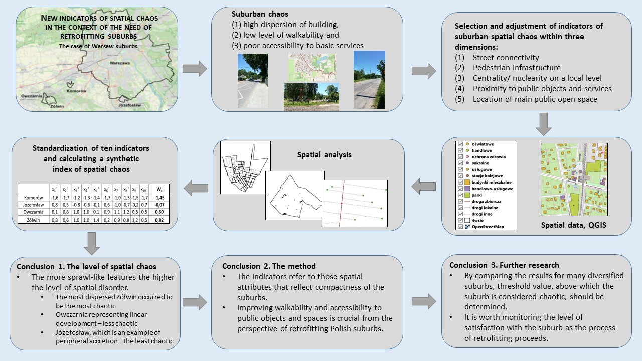
:The article is dedicated to the phenomenon of spatial chaos in the suburban areas of Polish cities, which, due to uncontrolled scattering of buildings (urban sprawl), require urgent retrofitting. These activities should contribute to the gradual densification of buildings and the more frequent functioning of suburbanites in the local environment, close to the place of residence. The authors claim that the retrofitting of suburbs can be accomplished by impacting two dimensions of spatial chaos: limited pedestrian mobility around the place of residence (walkability) and low access to basic services. The article proposes a set of ten indicators and a synthetic index of spatial chaos that allow measuring the level of disorder in particular suburbs, and therefore on a smaller scale than a municipality, and at the same time refer to the features of the living environment typical of Polish suburbs. These indicators are a direct reference to the abovementioned dimensions of suburban spatial chaos and allow to estimate the degree of compactness of suburban settlements in its functional aspect. The research proved that the more sprawl-like features, the higher the level of spatial disorder.
Keywords:
spatial chaos; compactness; walkability; accessibility; urban sprawl; retrofitting suburbs
1. Introduction
Spatial chaos is one of the main effects of spontaneous and mass suburbanization. The uncontrolled spread of buildings outside the boundaries of large cities, typical of post-socialist countries [1], is usually the result of a lack of appropriate tools for shaping spatial order, or inability to manage space development using existing tools. To capture what spatial chaos is, we should understand the essence of its dichotomous opposition, i.e., spatial order. When defining spatial order, The Spatial Planning and Land Development Act of 27 March 20031 emphasizes its two basic aspects: aesthetic and functional. This distinction confirms the earlier concept of Chojnicki [2], according to which spatial order expresses both the high aesthetic values of the space as well as its functionality, logic, readability, and clarity of structures, as well as the degree of harmonization with nature, high utility and efficiency in all spatial scales. Chojnicki emphasizes the importance of the spatial scale in which spatial order is considered, and this is reflected in three aspects in which analyses can be carried out [3]:
- physiognomic aspect (aesthetic, visual, architectural, compositional)—scale of the place (object, building, farm, place, street, nearest surroundings);
- morphological aspect (structural, local, urban, planning, landscape)—scale of the area (village, town, registration precinct, city, municipality, urban neighbourhood);
- functional aspect (regional, socioeconomic)—scale of the region (poviat or group of poviats, voivodship, historical lands, country).
The opposite of spatial order is spatial chaos, also referred to as disorder, disarray, disarrangement, and mess. All these concepts have a negative value and mean a violation of existing order or a lack of order where it should be [4]. Spatial chaos occurs when we deal with both unaesthetic and nonfunctional space [5]. Studying the manifestations of spatial chaos, we can experience methodological weaknesses and problems with the implementation of monitoring of dynamic changes that can be observed in the development of suburban space [6]. Most of the research on spatial order/chaos in Poland is carried out at the municipal level [7,8,9,10]. Studies ignore the same phenomena in a micro scale, for which not so much the lack of appropriate indicators as the methods of calculating them are problematic. These methods should be simple and possible to be used by persons responsible for shaping the municipal spatial policy.
The methods used in the research on spatial chaos are dominated by those based on indicators available in public statistics. Spatial order measured by the set of sustainable development indicators proposed and prepared by the UNDP (United Nations Development Program) is an example of such operationalization. The indicators are divided into four categories of order: environmental and spatial order, economic order, social order, and institutional and political order. There are studies where the total number of indicators selected within each of the partial orders can range from several dozen to even several hundred. An example of such studies is the research by Zioło [11], who analysed simultaneously 276 indicators of spatial order, and the research by Borys [12], who included up to 750 indicators. Such a large number of indicators limits perceptive possibilities and hinders the assessment of spatial order as a whole, hence it is suggested that their number should not exceed 30–40 [13].
The most frequently undertaken studies based on official statistics are aimed at determining areas (administrative units) of spatial order or spatial disorder [4,5], or conducting detailed analysis of one of its dimensions [13,14,15,16]. Polish public statistics allow to conduct analyses at the municipality level. However, public statistics cannot be used in the study of individual settlement units or their fragments. Research conducted on a micro scale requires a slightly different methodological approach. In this context, it is worth recalling the classic work of Galster et al. [17], who suggested how to measure the compactness of buildings. They proposed seven dimensions/indicators of sprawl: continuity, concentration, clustering, centrality, nuclearity, mixed uses, and proximity, all calculated for either one-mile-square grids or the one-half-mile-square grids as the geographic units of analysis. Each dimension consists of a continuum with low values representing more sprawl-like features. This method allows to estimate the scale of spatial chaos on a lower than municipality level. The research on spatial chaos can also be based on building compactness measures. According to Sudra [18], the area of such analysis may then be not only administrative units, but also functional units, concentric zones (rings) or sector zones, as well as a regular grid (e.g., squares). Some of these areas represent a lower level of analysis than the municipality. The search for new indicators can be inspired by the research on different dimensions and aspects of compactness, as manifestations of spatial order or chaos on a local scale.
The aim of the paper is to present a set of indicators that allow measuring the level of spatial chaos in the suburbs, i.e., on a smaller scale than the municipality. These indicators directly refer to the spatial chaos expressed by the low compactness of suburban settlement units in its functional aspect. A set of indicators will be tested in the study of four suburbs near Warsaw and the method will allow to estimate which of them is more and which is less chaotic. It is assumed that, in the case of urban sprawl, the level of chaos is the highest in suburbs that represent the most dispersed and extensive model of urban sprawl, and the least in urban villages adjacent to cities. The level of spatial chaos obtained for different types of urban sprawl will be referred to the village that is considered a sustainable suburb.
2. The Need of Rethinking Urban Sprawl—Review of Literature
2.1. Retrofitting of Suburbs by Increasing Their Compactness
Nowadays, in both developed countries and those trying to catch up with them, city outskirts are growing faster than their cores. This process is often spontaneous and not fully planned, which results in a redundant form of suburbanization called urban sprawl. In Central and Eastern European countries, including Poland, the 1990s were the beginning of extensive suburbanization, which resulted in many negative spatial and social effects called urban sprawl [19]. Urban sprawl is considered to be an example of spatial chaos in its functional aspect. It has been well recognized throughout Central and Eastern Europe [19,20,21,22,23,24,25,26]. In Polish literature, urban sprawl is usually characterized by: irrational spatial structures; dispersion; cultivating auto-dependence; disproportionately depleting energy, land, and water resources; social isolation; monofunctionality; and a considerable proportion of gated communities [1,27,28,29,30,31]. While urban sprawl almost always has negative connotations, compactness, in turn, is a key term in the context of preventing this phenomenon. Gordon and Richardson [32] defined compactness as high-density or monocentric development, while Ewing [33] emphasized some concentration of employment and housing, as well as some mixture of land uses. Although the concept of compactness has various aspects, most share the common theme: land being used intensively and the distance between different land uses and users being minimized [34]. This way of defining compactness is consistent with the concept of New Urbanism, which is considered an antidote to urban sprawl. New Urbanism stands for moderate density, grid-like street pattern, mix of residential and commercial land uses, distinct centres, and orientation to walking and transit rather than private automobiles [35]. The idea of compact city has been widely discussed not only in Anglo-Saxon countries but also in Poland, mainly in the context of creating sustainable cities, less often suburbs [36,37].
The negative effects of redundant suburbanization have become an impulse to take actions that are aimed at introducing the principles of New Urbanism to suburbs. This process is known as retrofitting of suburbs. Retrofitting is not only intensification, but also restructuring and transforming of urban fabric [38]. Literature abounds with examples of physical and functional transformations of suburbs—mainly American ones [39,40], or manuals giving instructions how to repair typical sprawl elements [38,41]. The process of retrofitting of suburbs may prove to be particularly important if we take into account changes in family status and housing preferences. Nowadays, less-expensive, denser, and better-connected neighbourhoods are increasingly favoured, especially by downsizing and starter households that choose urban living (young professionals, empty-nester seniors, immigrants) [42].
In Europe, just like in America, suburbs need regeneration of existing forms. Some European countries (e.g., the UK) have already made the effort of changing negative consequences of suburbanization [43], while others have not. Poland belongs to the second group. Comparing suburbs of post-socialist countries with their western counterparts, the former are more dense and less widespread [44], hence the need for retrofitting suburbs is particularly urgent in Central and Eastern Europe.
2.2. Indicators of Suburban Spatial Chaos in the Context of Compactness
Basing on different definitions, compactness may embrace three forms of built environment: monocentric and polycentric forms (the spatial structure-based definitions), and high-density form (the intensity-based definitions) [45]. Compactness is therefore based not only on density parameter, but also other detailed urban form characteristics. This research presents a slightly modified concept of suburban compactness, which may prove useful in fighting spatial chaos. It takes into account spatial attributes other than density that can be shaped by local authorities, developers, or housing cooperatives. It is assumed that suburban compactness can be shaped, on the one hand, by introducing infrastructure favouring walkability (walkability leads to greater spatial coherence and encourages densification of other than residential functions), and on the other hand, by better accessibility to public functions, which is more strategically locating public objects and public spaces in order to enhance using them by as many residents as possible (better accessibility results in more community cohesion, more social contacts, greater economic vitality).
This paper suggests five spatial attributes of suburban built environment that represent walkability and accessibility. They can be considered as dimensions of suburban disorder on a smaller than the municipality level: (1) street connectivity, (2) pedestrian infrastructure, (3) centrality/nuclearity, (4) proximity to public objects and services, (5) location of public open space.
2.2.1. Street Connectivity
Street network serves the purposes of connectivity, while connectivity is responsible for the quantity of destinations that is available within a given distance from a certain point [46]. Low connectivity reflects spatial chaos in a functional aspect, because it decreases accessibility to different destinations, discourages people from walking, impedes localizing public services in optimal places, and prevents the creation of nodal points of activity.
Ozbil et al. [47] distinguished four different approaches regarding description and evaluation of street connectivity, two of which can be used when developing indicators of spatial chaos. The first approach is based on the division into rectilinear, curvilinear, and cul-de-sac street layouts, represented by indicators, like the number of intersections or cul-de-sacs across the unit area. The second approach directly discusses the connectivity of street networks as a factor that affects accessibility and walking. This approach is expressed by the following measures: density of street intersections per area; block size per area; cul-de-sacs per area; proportion of four-way intersections; the ratio of intersections to cul-de-sacs; the average distance between intersections; or the links–nodes ratio. The last measure draws on the graph method, where nodes represent intersections and dead ends, and edges represent the street segments that link them [48,49,50,51].
2.2.2. Pedestrian Infrastructure
Pedestrian infrastructure is a basic indicator of walkability, which is defined as a suitability that the road environment offers to pedestrians. As personal safety is one of the basic features of a walkable road environment, sidewalks seems to be an essential component of good pedestrian design in areas where automobile traffic is more than minimal [52]. Galanis and Eliou [53] suggested measuring pedestrian infrastructure together with street furniture. Pedestrian infrastructure can be assessed by: sidewalk area (m2); road segment length (m); sidewalk maximum width (m); sidewalk minimum width (m); min/max sidewalk width (%); maximum unobstructed width (m); minimum unobstructed width (m); min/max unobstructed width (%); min unobstructed/max sidewalk width (%). Street furniture, in turn, is described by the ratio of the number of street furniture to the sidewalk length. A less time-consuming way to evaluate pedestrian design is developing scales, which requires field visits. One of the examples of such methods is the Pedestrian Friendliness Index (PFI) by Replogle [54], who suggested a scale for a sidewalks factor. The scale consists of six points and the corresponding ratings: (1) no sidewalks: 0; (2) discontinuous, narrow sidewalks: 0.05; (3) narrow sidewalks along all major streets: 0.15; (4) adequate sidewalks along all major streets: 0.25; (5) adequate sidewalks along most streets with some off-street paths: 0.35; (6) pedestrian district with sidewalks everywhere, pedestrian streets and auto restraints: 0.45. The scale is dedicated to cities where roads are paved and the street categories along with the width of pavements are more diversified. If it is to be used in the suburbs, it must be modified and take into account the fact that not all suburban roads are equipped with sidewalks, and some roads are still unpaved.
Centrality/Nuclearity
Centrality usually indicates the degree to which employment (or economic land use) is located close to the centres of cities and towns [55]. It is usually captured by the density of employment and its average distance from the city centre [56]. The centrality dimension was originally dedicated to metropolitan areas. It characterizes the degree of centralization and decentralization in general and, in particular, distinguishes among monocentric, polycentric, and decentralised sprawl forms [17]. Similar to centrality, nuclearity is the extent to which an urban area is characterized by a mononuclear (as opposed to a polynuclear) pattern of development. Centrality is a measure best suited to mononuclear urban areas, while nuclearity allows to measure the level of polynuclearity, representing the situation where the same activities are dispersed over several intensely developed places—centres [17].
In the case of residential suburbs, where centrality is analysed in a smaller than regional scale, specialized functions localized in CBD (Central Business District), such as financial centres, technology centres, retail, or manufacturing hubs, should be replaced with spaces and objects (units) important on a local scale: shops, catering points, social infrastructure, recreational areas, train stations, bus stops, job concentrations, etc. Some of them play a role of “third places,” which are defined by Oldenburg [57] as places where we spend our free time, meet friends, take a rest after professional work and housework. When it comes to the location of such units, there are two possible scenarios: a concentration of a range of services in one place (a “hub” of services), or scattered services across the suburb [58]. Which one is better? Despite the rule that the basic services should be as close as possible to the place of residence [59], their considerable dispersion is not conducive to the creation of vital spaces. If most of the retail and service points are concentrated in a few nodes of activity and little are located near the edge of the suburb or across its whole area, it encourages human presence in public space, stimulates walking, makes such nodes more vital and services more profitable. When studying centrality in a particular suburb, one should remember that suburban structure features a very local form of activity, limited to small-scale services. Suburban centres are more clusters of services within individual land parcels than fully formed public spaces with the function of services, which would have the potential to integrate the scattered housing development and create new contemporary centres [60]. By-product activity generated by the co-location of a diverse range of uses is of special importance when it comes to smaller centres [61], and these include suburban nodes of activity. In the case of suburban walkability, not only the existence of clusters of activity is important, but also the distance between individual uses across the suburb.
2.2.3. Proximity to Public Objects and Services
The mix of land use and physical proximity to different destinations is one of the factors encouraging walking. A neighbourhood is considered walkable if facilities and services are within 400–800 m of a resident’s home (5–10 min walking) [62]. According to Galster et al. [17], proximity is the degree to which different land uses are close to each other across an urbanized area. The longer the distance people have to overcome, the lower the proximity between two points in space and the more the dispersion of functions. In the case of suburbs, we can assess sprawl by measuring distance to main public objects. They perform an important spatial and social function only if they are located in the middle of the suburb.
There are several ideas on how to measure proximity. The simplest one relies on a straight-line distance—the shortest distance from Point A to Point B [63]. This indicator, however, does not consider that different destinations are not connected by straight lines, but rather through a road network. Therefore, it is better to treat proximity as a physical distance between two points, expressed in metres/kilometres by road. If we measure proximity between two specific uses only, we can assess the average distance from a given land use to all observations of another use [17] or a distance to the nearest object of a given function. In the case of monofunctional suburbs, we can compare distances between a house and a nearest grocery store, because it reflects the accessibility of basic services and indicates the willingness of residents to walk.
Proximity can be measured by distance and time. Some scholars claim that travel time is a better predictor of proximity than physical distance. The latter is significantly less important in explaining spatial behavior; that is why travel time is a popular measure of geographical distance, particularly in urban regions [64].
In the case of proximity, we can also use a weighting system. The simplest system is based on two values: a weight of 1 for units that are within the reach of the local environment and a weight of 0 for units that are outside the reach of the local environment [63]. The reach of the local environment can be measured by reasonable walking distances (5–10 minutes of walking).
2.2.4. Location of Main Public Open Space
When retrofitting suburbs, considerable efforts should be focused on public open spaces, defined by Kellett and Rofe [65] (p. 11) as “space within the urban environment which is readily accessible to the community regardless of its size, design or physical features, and which is intended for, primarily, amenity or physical recreation, whether active or passive.” Among different types of public open space (identified with parks by Cohen et al. [66]), local parks are of special importance due to their recreational (active and/or passive), ecological, and social functions. According to Kellett and Rofe [65], local parks cover the area of up to 2 ha, and according to Swanwick et al. [67], up to 1.2 ha. They are located within a walking distance from houses up to 0.4 km and equipped with an area for play. This category of parks includes gardens, sitting-out areas, children’s playgrounds, but also hard landscaped areas and public squares. According to Kellett and Rofe [65], however, open space is predominantly soft surfaced and covered by greenery. Parks (along with other public spaces) provide a favourite destination for walking trips in the suburbs [68], enhance aesthetics of neighbourhoods [69], and promote public life [70]. They provide settings where people can experience formal or informal social and ecological interactions, fundamental to building sustainable communities [71]. Open public space fulfils its social and recreational function if it is proximate to houses; however, proximity should be considered alongside connectedness issues. Suburbs are problematic in this issue, because, according to Frank et al. [72], Western cities abound in low-density suburbs with disconnected neighbourhood design. It applies also to Polish suburbs, where additionally recreational spaces often do not have a safe pedestrian access [73].
When searching for relevant indicators of suburban disorder, it is worth considering the walkable distance to proximate public open space, which is no more than 1.6–2 km [66], or specifying the type of location of the main public open space, especially when its accessibility is considered to be an attribute of the suburb as a whole. Some parameters regarding public open areas are also desired. In Poland, urban standards of the 1970s do not apply any more [74], so British ones can be used instead. Thompson [75] suggested 2.83 ha per 1000 residents, split into 1.62 ha for active and 1.21 ha for passive open space. These parameters were adopted after Raymond Unwin, the designer of Letchworth garden city and Hampstead garden suburbs. The provision of green open space for passive leisure is of special significance in cities, because it protects biodiversity, provides sustainable urban drainage, and reducessmog. In the suburbs, the split into space for physical activity (this space does not have to be green) and passive leisure (mainly green spaces) is not needed since greenery is provided mainly by private gardens.
3. Materials and Methods
3.1. Study Area
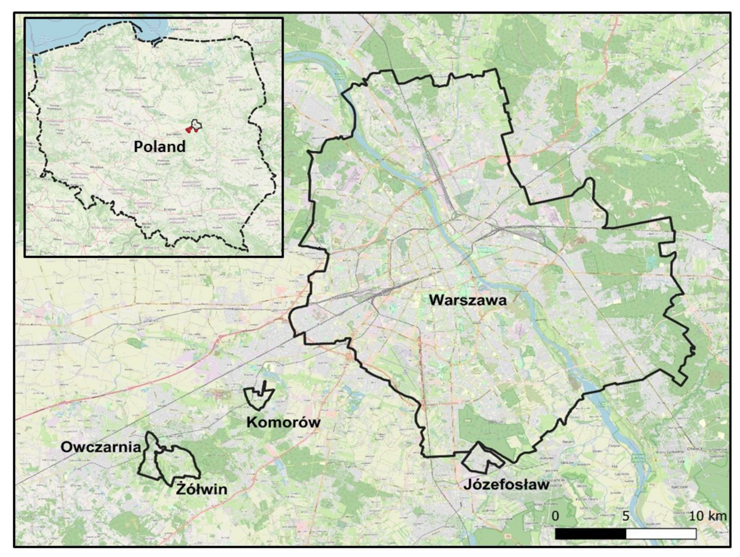
The study of spatial chaos was carried out in four suburbs located south or southwest of Warsaw, diversified in terms of density and type of buildings, road layout, accessibility to basic services and public spaces, and equipment with pedestrian infrastructure. Józefosław, Żółwin, and Owczarnia are examples of three different forms of urban sprawl, while Komorów is a model, rationally developed estate, that can be a reference suburb in the research on spatial chaos. The location of all four suburbs is presented in Figure 1.
- Józefosław: a typical urban village adjacent to Warsaw, populated in 2020 by 10,497 inhabitants,2 diversified in terms of type of buildings and type of housing estates, spontaneously developed along three main roads parallel to each other, dominated by gated communities and private cul-de-sacs. There is no local centre there and the pedestrian infrastructure and recreational spaces are still insufficient. The village represents the peripheral accretion type of urban sprawl.
- Żółwin and Owczarnia: two adjacent to each other former rural villages, populated in 2019 by 1637 inhabitants in Żółwin and 1455 inhabitants in Owczarnia,3 characterized by dispersed development, poor road and pedestrian infrastructure, and poor access to retail and services. Street layout in Żółwin consists of four intersecting main roads and departing from them cul-de-sacs, and Owczarnia extends along one main road with perpendicular cul-de-sacs on both sides. The whole area of Żółwin resembles a patchwork of houses, fields, and wasteland in between, while Owczarnia is an example of ribbon sprawl. Owczarnia represents linear development, while Żółwin the most dispersed type of urban sprawl.
- Komorów estate: a settlement modelled on a garden city, populated on 1st June 2020 by 3569 inhabitants,4 dominated by individual detached houses, whole settlement developed on a grid street layout around a local centre, equipped with pedestrian infrastructure and recreational spaces. Komorów estate is an example of sustainable suburbs.
3.2. Methods of Obtaining Data
It has been assumed that each of the five dimensions of spatial chaos (discussed earlier in the Introduction) should be represented by two indicators, so that each dimension is more comprehensively assessed. When determining values of particular indicators, the latest available spatial and demographic data were used. Due to the local nature of the studied phenomenon, it was decided to use detailed spatial data from several sources. The basic database was the Topographic Object Database (BDOT10k) from Polish geodetic and cartographic resources.5 The four villages studied are located in two poviats6: pruszkowski (Owczarnia, Żółwin, and Komorów) and piaseczyński (Józefosław). The village boundaries were downloaded from the administrative division units (ADMS) layer of BDOT10k database. Then, for individual poviats, data on roads, range of building, the buildings themselves, and location of point objects were selected and cut to the boundaries of individual villages.
A very important stage of processing the database was the identification of objects using the appropriate codes stored in the tables of attributes of individual layers. The “Classification of BDOT10k objects” being an attachment No. 2 to the Regulation of the Minister of Interior and Administration of 17 November 2011 concerning the database of topographic objects and the database of general geographic objects as well as the standard of cartographic studies, was used in this procedure. In the next step, data from the BDOT10k database were supplemented and verified using the Open Street Map (OSM spatial database). For the purpose of the study, vector data were downloaded from the OSM database, and the OSM map was used as the base map during the data verification process. Data sets on commercial and service objects as well as ranges of recreational areas turned out to be particularly useful.
In order to determine the location and function of some point objects necessary to set indicators, the object GeoSearch function available in the Google Maps and Google Earth applications was applied. In the Google Earth application, the selected objects were digitalized, then the data were transferred to the shapefile format with a simultaneous change of map projection.
Additionally, the Google Maps application with Street View service, and Open Street Map as the base map were used to verify the location, classification, and function of selected objects, and to identify pavements, cul-de-sacs, and intersections.
When identifying pavements, the latest orthophotomaps available at the national Geoportal (geoportal.gov.pl) were also used. Finally, the verification of the classification of spatial objects and their function necessary to assess the value of indicators was carried out during field studies.
All procedures related to the development of the spatial database, i.e., the collection and processing data from various sources, as well as determining spatial parameters needed to calculate eight out of ten chaos indicators were executed in the QGIS 3.4 program distributed under a free license.
In addition to the method and function of transforming and ordering spatial data sets, including several functions from the Geoprocessing Tools group, functions from the Geometry Tools groups, like Count points in polygon and Sum line lengths, were also used. In order to determine the centres of gravity of the villages and the centres of gravity of residential buildings, the Mean coordinates function was applied.
Clusters of commercial, service, and public facilities were determined using the DBSCAN7 clustering algorithm, having object locations previously transformed to points. The algorithm requires two parameters, a minimum cluster size (3 objects accepted), and the maximum distance allowed between clustered points (a distance of 100 m assumed).
The Centre of Gravity tool was applied to determine the centre of gravity of residential buildings and the Distance Matrix function was used to determine the distance. Most of the functions used are available in the module of Processing Toolbox Algorithms of QGIS.
Two out of ten indicators were assessed using special scales dedicated to this purpose: (4) pedestrian design and (9) location of the main local park. The scales were developed on the basis of existing scales that have been modified and one of them adapted to the suburban reality during pilot studies. The values of these two indicators were designated during field observations.
The list of individual indicators together with their justification and the databases they were obtained from is presented in Table 1.
3.3. Synthetic Indicator of Spatial Chaos
After collecting all the data, the level of mutual correlation of all ten indicators was checked; however, in the case of high correlation coefficients, the reduction in the number of indicators was not considered, because only two indicators were assigned to each of the five criteria (spatial chaos dimensions). Such a procedure would be advisable in the case of a larger number of indicators under each criterion. Additionally, the level of variability of individual indicators was determined using the coefficient of variation:
where:
- —the arithmetic mean value of the j-th indicator;
- —the value of standard deviation of the j-th indicator.
The low level of the coefficient of variation (below 10%) proves that the variable is quasi-constant and cannot be a good diagnostic feature, because it does not provide significant information about the phenomenon under study.
Synthetic indicators of spatial chaos were calculated using two alternative model-less methods (Komorów cannot be considered a model suburb although it has been assumed that its level of chaos should be very low). The first method is based on Perkal synthetic indicator [76,77], which is estimated as the arithmetic mean of traits (in this case, standardized indicators). A higher value means a higher position of the suburb in terms of its level of chaos. It is expressed by the formula:
where:
- n—the number of included indicators;
- —the standardized value of the j-th indicator of the i-th suburb:
- —the original value of the j-th indicator of the i-th suburb;
- —the arithmetic mean value of the j-th indicator;
- —the value of standard deviation of the j-th indicator.
The second method of calculating synthetic measures is based on zero unitarization algorithm of normalizing the original values of indicators, according to the formulas:
where:
- —the original value of the j-th indicator of the i-th suburb;
- —the minimum value in the set of values of a given indicator;
- —the maximum value in the set of values of a given indicator.
Compared to the standardization used in Perkal synthetic indicator, the zero unitarization method meets most of the normalization requirements [78]. Normalized diagnostic indicators are positive and take values from the same interval (0, 1), which allows for their aggregation. Ultimately, it allows for the construction of a synthetic measure, which can take two forms: unweighted (7) and weighted (8) mean of normalized indicators:
where:
- n—the number of included indicators;
- —the normalized value of the j-th indicator of the i-th suburb;
- —the weighting factor of the j-th indicator, assuming that all weighting factors add up to 1.
To determine the weighting factors () of diagnostic features (ten indicators), the entropy weighting method was used. The method proceeds in the following stages [79,80]:
- Calculating the entropy of the j-th indicator as follows:where:
- m—number of objects (suburbs);
- ;
- (when , make ).
- Calculating the entropy weight of the j-th indicator as follows:where:
- 0 ≤ ≤ 1 and .
4. Results
In the first stage of the empirical research, the degree of mutual correlation of the indicators and the degree of their variability were checked. Most indicators are strongly correlated with each other, partly due to the multi-criteria nature of the problem under study, where criteria are not required to be independent of each other. When it comes to the coefficients of variation, the variability of all indictors is significant (ten values are above 10%), so indicators under study can be considered good diagnostic features of spatial chaos (Table 2).
In the next stage, a weighting system was applied to the indicators. Table 2 shows that none of the ten indicators is a powerful driving force of spatial chaos. It turned out that the most important indicator was straight-line distance from the centre of gravity of the suburb to the nearest public object (0.163), which represents proximity dimension of spatial disorder. The second-most significant contributor is the length of public roads equipped with pavement in relation to the total length of roads (pedestrian infrastructure dimension).
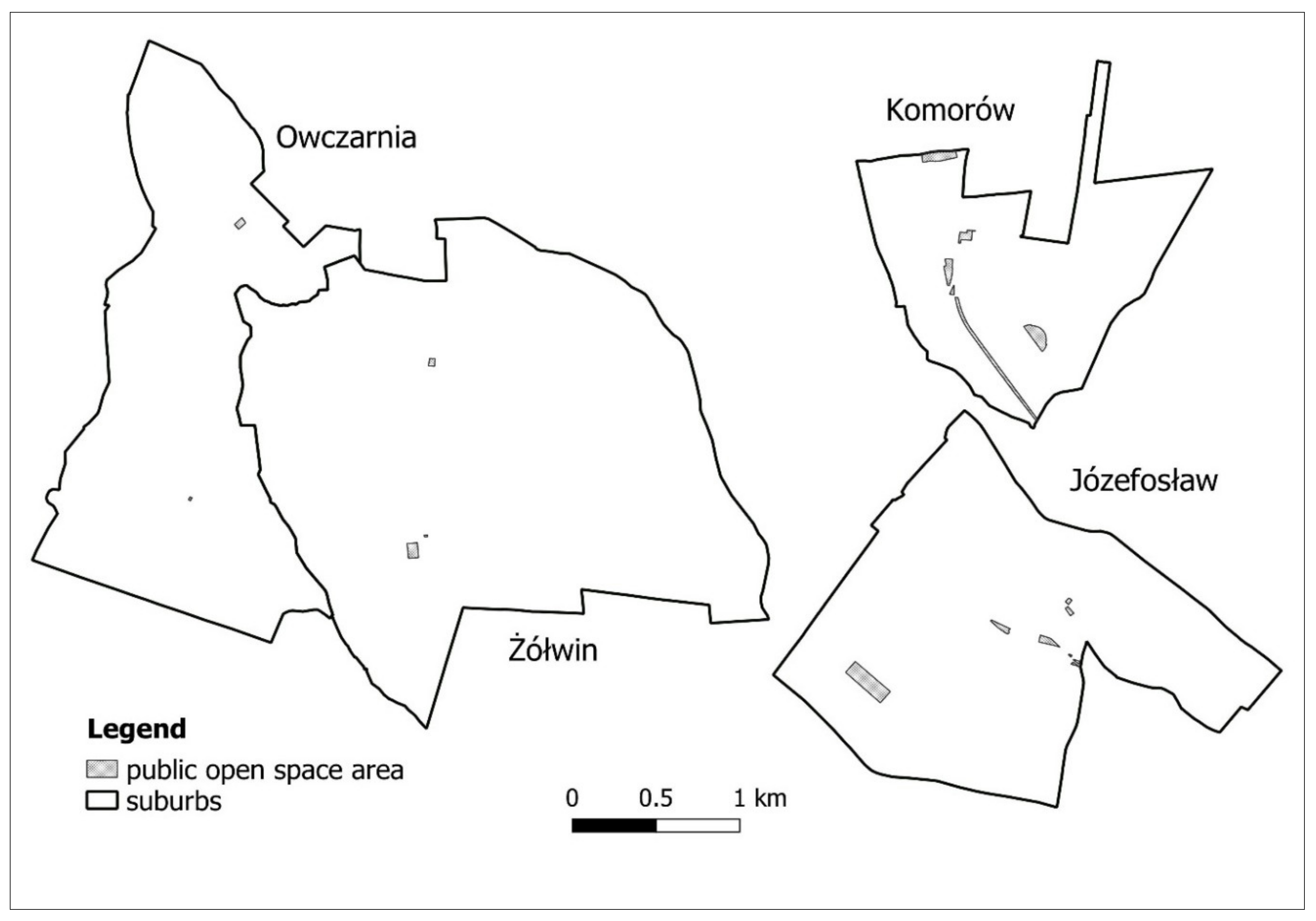
The study was comparative in its character. Table 3 shows original values of particular indicators as well as three synthetic measures of spatial chaos, and Figure 2, Figure 3 and Figure 4 spatial parameters necessary to calculate some of the indicators. All three synthetic measures unambiguously define the order of the suburbs in terms of the level of spatial chaos. The difference between the weighted and unweighted synthetic measure is minimal since there are no pronounced differences between weighting factors. None of the indicators seem to be of particular importance. This implies that weighting does not always significantly affect the final result.
The selection of indicators allowed to differentiate individual suburbs in terms of the level of spatial chaos. The analysis has confirmed that, regardless of the method of calculating the synthetic indicator, the lowest value is characteristic for Komorów, which was assumed to be the least chaotic among the suburbs studied. All destimulants for Komorów have noticed the highest values, which indicates the least sprawl-like features measured by individual indicators. Only in the case of the straight-line distance from the centre of gravity of the suburb to the nearest public object, Józefosław has scored better than Komorów, but this is due to unusual course of the northeastern border of the Komorów estate, which disturbs the compactness of the whole suburb. The difference in values between Komorów and Józefosław—the next in ascending order—is significant. The hypothesis has been confirmed: considering three suburbs that represent different types of urban sprawl, Żółwin—the most dispersed suburb—has obtained the highest value of spatial disorder, and Józefosław, representing the peripheral accretion model of development, the lowest. The level of chaos in Józefosław is affected by a relatively low density of the public road network due to a high proportion of internal cul-de-sacs belonging to gated communities, and the smallest area of public open space per 1000 residents comparing to other suburbs, since the pace of development here is very fast and the municipality did not reserve land for public space in previous local plans. Żółwin, in turn, represents the most sprawl-like suburbs mainly because of low level of nuclearity and peripheral location of the main recreational area, which is a consequence of a high dispersion of housing and planning neglect in the past.
5. Conclusions and Discussion
The study has opened new possibilities of measuring the level of spatial chaos on a local scale. The indicators were intended to refer to those spatial attributes that reflect compactness of the suburbs and can be shaped by local authorities, developers, or housing cooperatives. It was assumed that improving walkability and accessibility to public objects and spaces is crucial from the perspective of retrofitting suburbs. The test of the method described in this paper confirmed that spatial chaos is closely linked to the type of urban sprawl. The more sprawl-like features, the higher the level of spatial disorder. Żółwin, which represents the most extensive, spontaneous, and negative form of development, turned out to be the most chaotic, and Komorów the most sustainable suburb. The fact that the hypothesis has been confirmed proves the validity of the set of indicators constructed for the research. The study, however, has also revealed weaknesses of the method and pointed out several issues that are worth considering when drawing general conclusions.
The method is universal and can be used in various types of built-up areas. However, the calculation of some spatial parameters is limited in the case of gated housing estates as well as recreational areas and playgrounds not accessible to the public, hence the necessity to exclude gated communities from this type of research. Another complication is the functioning of suburbanites, who do not respect administrative boundaries. Borders are not a barrier in making decisions as to which grocery or supermarket to choose, so one of the indicators had to be modified to better reflect the functioning of the residents. The proposed methodology is therefore more effective in the case of remote and separated settlements than suburbs belonging to a larger area of continuous development.
The synthetic measure of spatial chaos strongly depends on the set of individual indicators and assumptions adopted for each of them. Some weaknesses of the method result from parameters included in particular measures. One such limitation is a strong impact of the shape of the suburb on the score of indicators based on geometric calculations. Another simplification is the exclusion of the area of commercial and service facilities and calculating clusters only on the basis of the number of points. There may also be difficulties in classifying some walking areas as local parks according to the definition presented in this paper. All these constraints, however; should be considered as a typical element of the indicator construction process, which requires certain assumptions and, consequently, also simplifications.
When it comes to the technical side of the research, QGIS and its functions proved to be a good tool for determining indicators of spatial chaos and a topographic database on a scale of 1:10,000 useful in determining spatial characteristics on a local scale.
The method can be further modified. By comparing the results for various suburbs, including settlements that are a manifestation of spatial order, each indicator can be assigned a threshold value, above which the way the space is developed will be considered chaotic. Spatial chaos can also be gradated as low, medium, and high by matching the appropriate range of synthetic indicator values to each of the three levels. All this, however, requires investigating a significant number of suburbs.
The method tested in this study can be applied in monitoring the process of retrofitting suburbs. Retrofitting, however, should be perceived not only as an improvement of physical space, but also as an impulse to increase the level of life satisfaction among suburbanites. According to Neuman [82], an attempt to make suburban areas sustainable only by shaping their urban form is usually ineffective. Taking into account contemporary development paradigm, which is based mostly on the quality of life, the increase in neighbourhood satisfaction, and thus overall life satisfaction, should be one of the purposes of all the changes made in space. Other research show that some physical design characteristics, like the dominance of traditional grid-layout neighbourhoods over cul-de-sac streets, have a greater role in determining neighbourhood satisfaction in low-density suburbs than sociodemographic factors [83].
If the method presented in this paper were supplemented with the research on the usage of pedestrian infrastructure as well as local parks, shops, and public objects, it would be possible to determine whether, with the decrease in spatial chaos, the suburban public spaces and objects are more frequently used by the residents. It is also worth monitoring the level of satisfaction with the place of residence as changes in space proceed.
To conclude, this study should be seen as the first step in a comprehensive research project on the possibilities, needs, changes, and perception of the process of making Polish suburbs more compact, walkable, and community-friendly.
Author Contributions
Conceptualization, D.M.; Data curation, W.P.; Formal analysis, D.M. and W.P.; Investigation, D.M. and W.P.; Methodology, D.M. and W.P.; Software, W.P.; Supervision, D.M.; Writing—original draft, D.M. All authors have read and agreed to the published version of the manuscript.
Funding
The publication of the article was financed by the Faculty of Geography and Regional Studies, University of Warsaw.
Conflicts of Interest
The authors declare no conflict of interest.
References
- Mantey, D. Żywiołowość Lokalizacji Osiedli Mieszkaniowych Na Terenach Wiejskich Obszaru Metropolitalnego Warszawy; Uniwersytet Warszawski, WGiSR: Warsaw, Poland, 2011. [Google Scholar]
- Chojnicki, Z. Współczesne problemy gospodarki przestrzennej. In Współczesne Problemy Geografii Społeczno-Ekonomicznej Polski; Chojnicki, Z., Czyż, T., Eds.; Wydawnictwo Naukowe UAM: Poznań, Poland, 1992; pp. 9–19. [Google Scholar]
- Kozłowski, L.; Bielska, B.; Brzezińska-Rawa, A.; Flanz, S.; Goszczyński, W.; Karwacki, A.; Knieć, W.; Koziński, G.; Kurowska, I.; Marcysiak, T.; et al. Ład Przestrzenny w Województwie Kujawsko-Pomorskim. Diagnoza z Założeniami Programu Jego Kształtowania; UMK in Toruń, Wydział Nauk o Ziemi, Urząd Marszałkowski Województwa Kujawsko-Pomorskiego in Toruń Departament Rozwoju Regionalnego: Toruń, Poland, 2016. [Google Scholar]
- Kopeć, A. Poziom ładu przestrzennego w podmiejskiej strefie aglomeracji Trójmiasta. Kategoria społeczna i legislacja. In Gospodarka Przestrzenna Społeczeństwu; Ratajczak, W., Stachowiak, K., Eds.; Bogucki Wydawnictwo Naukowe: Poznań, Poland, 2010; pp. 123–143. [Google Scholar]
- Falkowski, J. Ład przestrzenny w planowaniu i zagospodarowaniu obszarów wiejskich na przykładzie województwa kujawsko-pomorskiego. Studia Obsz. Wiej. 2018, 50, 25–47. [Google Scholar] [CrossRef]
- Śleszyński, P. Wskaźniki Zagospodarowania i Ładu Przestrzennego w Gminach; Biuletyn KPZK PA: Warsaw, Poland, 2013; Volume 252. [Google Scholar]
- Ślęzak, T.; Zioło, Z. Społeczno-Gospod. I Przyr. Asp. Ładu Przestrz; Biuletyn KPZK PAN: Warsaw, Poland, 2003; Volume 205. [Google Scholar]
- Wdowicka, M.; Mierzejewska, L. Chaos w zagospodarowaniu przestrzennym stref podmiejskich jako efekt braku zintegrowanego systemu planowania (na przykładzie strefy podmiejskiej Poznania). Probl. Rozw. Miast 2012, 1, 40–52. [Google Scholar]
- Gorzelak, G. Szkic o wymiarach ładu przestrzennego. In Społeczno-Gospodarcze i Przyrodnicze Aspekty Ładu Przestrzennego; Ślęzak, T., Zioło, Z., Eds.; Biuletyn KPZK PAN: Warsaw, Poland, 2003; Volume 205, pp. 55–69. [Google Scholar]
- Śleszyński, P.; Markowski, T.; Kowalewski, A. Studia nad Chaosem Przestrzennym. Tom 3. Synteza. Uwarunkowania, Skutki i Propozycje Naprawy Chaosu Przestrzennego; Studia KPZK PAN: Warsaw, Poland, 2018; Volume 182. [Google Scholar]
- Zioło, Z. Przestrzeń geograficzna jako miejsce realizacji idei ładu przestrzennego. In Społeczno-Gospodarcze i Przyrodnicze Aspekty Ładu Przestrzennego; Ślęzak, T., Zioło, Z., Eds.; Biuletyn KPZK PAN: Warsaw, Poland, 2003; Volume 205, pp. 25–43. [Google Scholar]
- Borys, T. Wskaźniki Zrównoważonego Rozwoju; Wyd. Ekonomia i Środowisko: Warsaw-Białystok, Poland, 2005. [Google Scholar]
- Śleszyński, P. Propozycja kompleksowej koncepcji wskaźników zagospodarowania i ładu przestrzennego. In Wskaźniki Zagospodarowania i Ładu Przestrzennego w Gminach; Śleszyński, P., Ed.; Biuletyn KPZK PAN: Warsaw, Poland, 2013; Volume 252, pp. 176–231. [Google Scholar]
- Affek, A. Propozycje wskaźników środowiskowych do oceny zagospodarowania i ładu przestrzennego w gminach. In Wskaźniki Zagospodarowania i Ładu Przestrzennego w Gminach; Śleszyński, P., Ed.; Biuletyn KPZK PAN: Warsaw, Poland, 2013; Volume 252, pp. 51–86. [Google Scholar]
- Rosik, P.; Ciechański, A. Propozycje wskaźników infrastruktury transportu drogowego i kolejowego. In Wskaźniki Zagospodarowania i Ładu Przestrzennego w Gminach; Śleszyński, P., Ed.; Biuletyn KPZK PAN: Warsaw, Poland, 2013; Volume 252, pp. 110–131. [Google Scholar]
- Górczyńska, M. Wskaźniki zagospodarowania i ładu przestrzennego w miastach i na obszarach silnie zurbanizowanych. In Wskaźniki Zagospodarowania i Ładu Przestrzennego w Gminach; Śleszyński, P., Ed.; Biuletyn KPZK PAN: Warsaw, Poland, 2013; Volume 252, pp. 87–109. [Google Scholar]
- Galster, G.; Hanson, R.; Ratcliffe, M.R.; Wolman, H.; Coleman, S.; Freihage, J. Wrestling Sprawl to the Ground: Defining and Measuring an Elusive Concept. Hous. Policy Debate 2001, 12, 681–717. [Google Scholar] [CrossRef]
- Sudra, P. Zastosowanie wskaźników koncentracji przestrzennej w badaniu procesów urban sprawl. Przegląd Geogr. 2016, 88, 247–272. [Google Scholar] [CrossRef]
- Stanilov, K.; Sýkora, L. Confronting Suburbanization Urban Decentralization in Postsocialist Central and Eastern Europe; John Wiley & Sons: Chichester, UK, 2014. [Google Scholar]
- Tsenkova, S.; Nedović-Budić, Z. The Urban. Mosaic of Post-Socialist Europe: Space, Institutions and Policy; Physica-Verlag: New York, NY, USA, 2006. [Google Scholar]
- Sykora, L.; Ourednicek, M. Sprawling Post-Communist Metropolis: Commercial and Residential Suburbanisation in Prague and Brno, the Czech Republic. Employment Deconcentration in European Metropolitan Areas: Market. Forces versus Planning Regulations; Dijst, M., Razin, E., Vazquez, C., Eds.; Springer: Dordrecht, The Netherlands, 2007; pp. 209–234. [Google Scholar]
- Pichler-Milanović, N.; Gutry-Korycka, M.; Rink, D. Sprawl in the Post-Socialist City: The Changing Economic and Institutional Context of Central and Eastern European Cities; Couch, C., Petschel-Held, G., Leontidou, L., Eds.; Urban Sprawl in Europe, Landscape, Land-Use Change and Policy; Wiley-Blackwell: Hoboken, NY, USA, 2007; pp. 102–135. [Google Scholar]
- Tammaru, T.; Leetmaa, K.; Silm, S.; Ahas, R. Temporal and Spatial Dynamics of the New Residential Areas Around Tallinn. Eur. Plan. Stud. 2009, 17, 423–439. [Google Scholar] [CrossRef] [Green Version]
- Hirt, S. Iron Curtains: Gates, Suburbs and Privatization of Space in the Post-Socialist City; Wiley-Blackwell: Oxford, UK; Malden, MA, USA, 2012. [Google Scholar]
- Dinić, M.; Mitković, P. Suburban design: From “bedroom communities” to sustainable neighborhoods. Geod. Vestn. 2016, 60, 98–113. [Google Scholar] [CrossRef]
- Taubenböck, H.; Gerten, K.; Rusche, K.; Siedentop, S.; Wurm, M. Patterns of Eastern European urbanisation in the mirror of Western trends—Convergent, unique or hybrid? Environ. Plan. B Urban Anal. City Sci. 2019, 46, 1206–1225. [Google Scholar] [CrossRef] [Green Version]
- Springer, F. Wanna z Kolumnadą; Wyd. Czarne: Wołowiec, Poland, 2013. [Google Scholar]
- Zuziak, Z. Strefa podmiejska w architekturze miasta. W stronę nowej architektoniki regionu miejskiego. In Problem Suburbanizacji; Lorens, P., Ed.; Urbanista: Warsaw, Poland, 2005; pp. 17–32. [Google Scholar]
- Chmielewski, J.M. Problemy rozpraszania się zabudowy na obszarze metropolitalnym Warszawy. In Problem Suburbanizacji; Lorens, P., Ed.; Urbanista: Warsaw, Poland, 2005; pp. 52–62. [Google Scholar]
- Solarek, K. Struktura Przestrzenna Strefy Podmiejskiej Warszawy: Determinanty Współczesnych Przekształceń; Politechnika Warszawska: Warsaw, Poland, 2013. [Google Scholar]
- Zimnicka, A.; Czernik, L. Kształtowanie Przestrzeni Wsi Podmiejskiej Raport z Badań Obszaru Oddziaływania Miasta Szczecin; Hogben: Szczecin, Poland, 2007. [Google Scholar]
- Gordon, P.; Richardson, H.W. Are compact cities a desirable planning goal? J. Am. Plan. Assoc. 1997, 63, 95–106. [Google Scholar] [CrossRef]
- Ewing, R. Is Los Angeles-style sprawl desirable? J. Am. Plan. Assoc. 1997, 63, 107–126. [Google Scholar] [CrossRef]
- Ahlfedlt, G.; Pietrostefani, E. The Effects of Compact Urban form: A Qualitative and Quantitative Evidence Review; Coalition for Urban Transitions: London, UK; Washington, DC, USA, 2017; Available online: http://newclimateeconomy.net/content/cities-working-papers (accessed on 9 July 2020).
- Fulton, W. The New Urbanism: Hope or Hype for American Communities; Lincoln Institute of Land Policy: Cambridge, MA, USA, 1996. [Google Scholar]
- Polit, A. Idea miasta zwartego a rzeczywistość. Czas. Tech. Archit. 2010, 14, 85–91. [Google Scholar]
- Mierzejewska, L. Miasto zwarte, rozproszone, zrównoważone. Studia Miej. 2015, 19, 9–22. [Google Scholar]
- Dunham-Jones, H.; Willianson, J. Retrofitting Suburbia: Urban. Design Solutions for Redesigning Suburbs; John Wiley & Sons: Hoboken, NJ, USA, 2009. [Google Scholar]
- Marique, A.F.; Reiter, S. Retrofitting the Suburbs: Insulation, density, urban form and location. Environ. Manag. Sustain. Dev. 2014, 3, 138–153. [Google Scholar] [CrossRef] [Green Version]
- Talen, E. Retrofitting Sprawl: Addressing Seventy Years of Failed Urban Form; University of Georgia Press: Athens, GA, USA, 2015. [Google Scholar]
- Tachieva, G. Sprawl Repair Manual; Island Press: Washington, DC, USA, 2010. [Google Scholar]
- Fishman, R. Longer view: The fifth migration. J. Am. Plan. Assoc. 2005, 71, 357–366. [Google Scholar] [CrossRef]
- ODPM (Office of the Deputy Prime Minister). Sustainable Communities: Building for the Future; ODPM: London, UK, 2003.
- Stanilov, K. The Post-Socialist City: Urban form and Space Transformations in Central and Eastern Europe after Socialism; Springer: Dordrecht, The Netherlands, 2007. [Google Scholar]
- Tsai, Y.-H. Quantifying Urban Form: Compactness versus ‘Sprawl’. Urban. Stud. 2005, 42, 141–161. [Google Scholar] [CrossRef]
- Trova, V. Measures of Street Connectivity: Spatialist Lines (MoSC). In Accessibility Instruments for Planning Practice; Hull, A., Silva, C., Bertolini, L., Eds.; COST Office: Porto, Portugal, 2012; pp. 103–109. [Google Scholar]
- Ozbil, A.; Peponis, J.; Stone, B. Understanding the link between street connectivity, land use and pedestrian flows. Urban. Des. Int. 2011, 16, 125–141. [Google Scholar] [CrossRef]
- Barthelemy, M.; Flammini, A. Modeling Urban Street Patterns. Phys. Rev. Lett. 2008, 100, 138702. [Google Scholar] [CrossRef] [Green Version]
- Cardillo, A.; Scellato, S.; Latora, V.; Porta, S. Structural properties of planar graphs of urban street patterns. Phys. Rev. E 2006, 73. [Google Scholar] [CrossRef] [Green Version]
- Lin, J.; Ban, Y. Complex network topology of transportation systems. Transp. Rev. 2013, 33, 658–685. [Google Scholar] [CrossRef]
- Marshall, S.; Gil, J.; Kropf, K.; Tomko, M.; Figueiredo, L. Street network studies: From networks to models and their representations. Netw. Spat. Econ. 2018, 15. [Google Scholar] [CrossRef] [Green Version]
- Parks, J.R.; Schofer, J.L. Characterizing neighborhood pedestrian environments with secondary data. Transp. Res. Part. D Transp. Environ. 2006, 11, 250–263. [Google Scholar] [CrossRef]
- Galanis, A.; Eliou, N. Evaluation of the pedestrian infrastructure using walkability indicators. Wseas Trans. Environ. Dev. 2011, 12, 385–394. [Google Scholar]
- Replogle, M. Computer transportation models for land use regulation and master planning in Montgomery County, MD. Transp. Res. Rec. 1990, 1262, 91–100. [Google Scholar]
- Razin, E.; Dijst, M.; Vázquez, C. Employment Deconcentration in European Metropolitan Areas: Market Forces versus Planning Regulations; Springer: Dordrecht, Germany, 2007. [Google Scholar]
- Anas, A.; Arnott, R.; Small, K.A. Urban Spatial Structure. J. Econ. Lit. 1998, 36, 1426–1464. [Google Scholar]
- Oldenburg, R. The Great Good Place: Cafes, Coffee Shops, Bookstores, Bars, Hair Salons, and Other Hangouts at the Heart of a Community; Marlow & Co.: New York, NY, USA, 1999. [Google Scholar]
- Boulange, C.; Pettit, C.; Giles-Corti, B. The Walkability Planning Support System: An Evidence-Based Tool to Design Healthy Communities. In Planning Support Science for Smarter Urban Futures; Geertman, S., Allan, A., Pettit, C., Stillwell, J., Eds.; Springer International Publishing: Cham, Switzerland, 2017; pp. 153–166. [Google Scholar]
- Glaeser, E.L. Agglomeration Economics; The University of Chicago Press: Chicago, IL, USA, 2010. [Google Scholar]
- Bajwoluk, T. Centres in suburban zones—The form and accessibility. Czas. Tech. Archit. 2015, 12-A, 241–257. [Google Scholar]
- Vaughan, L.; Emma Jones, C.; Griffiths, S.; Haklay, M. The spatial signature of suburban town centres. J. Space Syntax 2010, 1, 77–91. [Google Scholar]
- Talen, E.; Koschinsky, J. The walkable neighborhood: A literature review. Int. J. Sustain. Land Use Urban. Plan. 2013, 1, 42–63. [Google Scholar] [CrossRef]
- Roberto, E. The Spatial Proximity and Connectivity (SPC) Method for Measuring and Analyzing Residential Segregation. Sociol. Methodol. 2018, 48, 182–224. [Google Scholar] [CrossRef] [Green Version]
- MacEachren, A.M. Travel time as the basis of cognitive distance. Prof. Geogr. 1980, 32, 30–36. [Google Scholar] [CrossRef]
- Kellett, J.; Rofe, M.W. Creating Active Communities: How can Open and Public Spaces in Urban and Suburban Environments Support Active Living? A Literature Review. Report by the Institute for Sustainable Systems and Technologies; University of South Australia to SA Active Living Coalition: Adelaide, SA, Australia, 2009; Available online: https://www.healthyactivebydesign.com.au/images/uploads/Creating_Active_Communities_electronic_FINAL.pdf (accessed on 8 July 2020).
- Cohen, D.; McKenzie, T.; Sehgal, A.; Williamson, S.; Golinelli, D.; Lurie, N. Contribution of public parks to physical activity. Am. J. Public Health 2007, 97/3, 509–514. [Google Scholar] [CrossRef]
- Swanwick, C.; Dunnett, N.; Woolley, H. Nature, Role and Value of Green Space in Towns and Cities: An Overview. Built Environ. 2003, 29, 94–106. [Google Scholar] [CrossRef]
- Tilt, J.H. Walking Trips to Parks: Exploring Demographic, Environmental Factors, and Preferences for Adults with Children in the Household. Prev. Med. 2010, 50, 69–73. [Google Scholar] [CrossRef] [PubMed]
- Walker, C. The Public Value of Urban Parks. In Beyond Recreation: A Broader View of Urban Parks; The Urban Institute: Washington, DC, USA, 2004; Available online: https://www.wallacefoundation.org/knowledge-center/Documents/The-Public-Value-of-Urban-Parks.pdf (accessed on 9 July 2020).
- Duany, A.; Plater-Zyberk, E.; Speck, J. Suburban Nation: The Rise of Sprawl and the Decline of the American Dream; North Point Press: New York, NY, USA, 2000. [Google Scholar]
- Chiesura, A. The Role of Urban Parks for the Sustainable City. Landsc. Urban. Plan. 2004, 68, 129–138. [Google Scholar] [CrossRef]
- Frank, L.; Andersen, M.; Schmid, T. Obesity relationships with community design, physical activity, and time spent in cars. Am. J. Prev. Med. 2004, 27, 87–96. [Google Scholar] [CrossRef] [PubMed]
- Mantey, D. Wzorzec Miejskiej Przestrzeni Publicznej w Konfrontacji z Podmiejską Rzeczywistością; Wydawnictwa Uniwersytetu Warszawskiego: Warsaw, Poland, 2019. [Google Scholar]
- Dąbrowska-Milewska, G. Standardy urbanistyczne dla terenów mieszkaniowych: Wybrane zagadnienia. Archit. Artibus 2010, 2, 17–31. [Google Scholar]
- Thompson, S. Design for Open Space. Fact Sheet; Your Development: Melbourne, VIC, Australia, 2008. Available online: http://yourdevelopment.org/factsheet/view/id/72 (accessed on 14 April 2009).
- Perkal, J. O wskaźnikach antropologicznych. Przegląd Antropol. 1953, 19, 210–221. [Google Scholar]
- Czyż, T. Metoda wskaźnikowa w geografii społeczno-ekonomicznej. Rozw. Reg. I Polityka Reg. 2016, 34, 9–19. [Google Scholar]
- Kukuła, K. Metoda unitaryzacji zerowanej (Zero Unitarisation Method); PWN: Warsaw, Poland, 2000. [Google Scholar]
- Tomal, M. Moving towards a Smarter Housing Market: The Example of Poland. Sustainability 2020, 12, 683. [Google Scholar] [CrossRef] [Green Version]
- Wand, Q.; Mao, Z.; Xian, L.; Liang, Z. A study on the coupling coordination between tourism and the low-carbon city. Asia Pac. J. Tour. Res. 2019, 24, 550–562. [Google Scholar] [CrossRef]
- Whyte, W.H. The Social Life of Small Urban Spaces; The Municipal Arts Society: New York, NY, USA, 1980. [Google Scholar]
- Newman, M. The Compact City Fallacy. J. Plan. Educ. Res. 2005, 25, 11–26. [Google Scholar] [CrossRef]
- Abass, Z.I.; Andrews, F.; Tucker, R. Socializing in the suburbs: Relationships between neighbourhood design and social interaction in low-density housing contexts. J. Urban. Des. 2020, 25, 108–133. [Google Scholar] [CrossRef]
| 1 | Act regulating issues related to planning of Polish space and introducing rules for its development; setting out the type, scope, and procedures for enacting planning documents at different levels of administration; and defining new categories of space, e.g., area of public space, and new conceptual categories, e.g., spatial order. |
| 2 | Data retrieved from the website of the municipality of Piaseczno: http://bip.piaseczno.eu/artykul/55/4150/demografia. |
| 3 | Both data sources retrieved from the website of the municipality of Brwinów: https://bip.brwinow.pl/gmina-brwinow-w-liczbach. |
| 4 | Data obtained from the Citizens’ Affairs Department of the municipality of Michałowice. |
| 5 | The topographic database obtained for the WGSR UW from the Central Office of Geodesy and Cartography. |
| 6 | Poviat is the second-level unit of local government and administration in Poland between a municipality (local level) and a voivodeship (regional level). |
| 7 | DNSCAN—Density-based spatial clustering of applications with noise. It is a density-based clustering algorithm: given a set of points in some space, it groups together points that are closely packed together (points with many nearby neighbors). |
| 8 | Cul-de-sacs are dead-end streets among the category of “other” roads according to the topographic database. |
| 9 | The value of the indicator does not depend on whether the pavement is on one or both sides of the road. |
| 10 | Units of other than residential function: bars, restaurants, banks, cash machines, pharmacies, shops, schools, post offices, local community centres. |
| 11 | Cluster is a concentration of a minimum three units of other than residential function at a distance of not more than 100 m from each other. |
| 12 | Centre of gravity is a point determining the mass centre of geometry of surface objects. |
| 13 | It was assumed that the nearest grocery does not have to be within the studied suburb, it can be located in a neighbouring administrative unit. |
| 14 | The main public open space is the largest in size. |
| 15 | Node of activity is identified with a cluster. |
Figure 1.
Location of the suburbs studied.

Figure 2.
Public roads equipped with pavement.
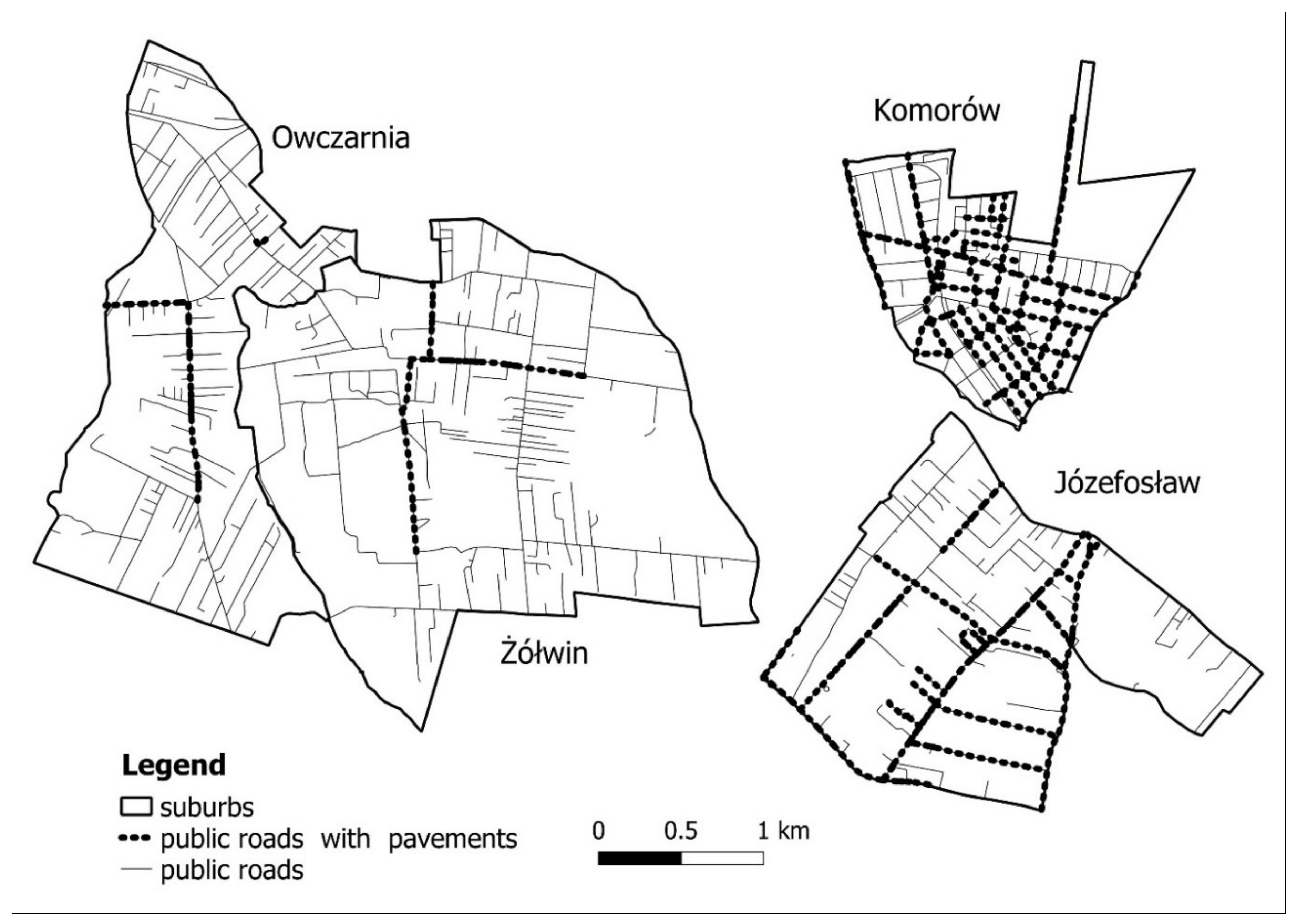
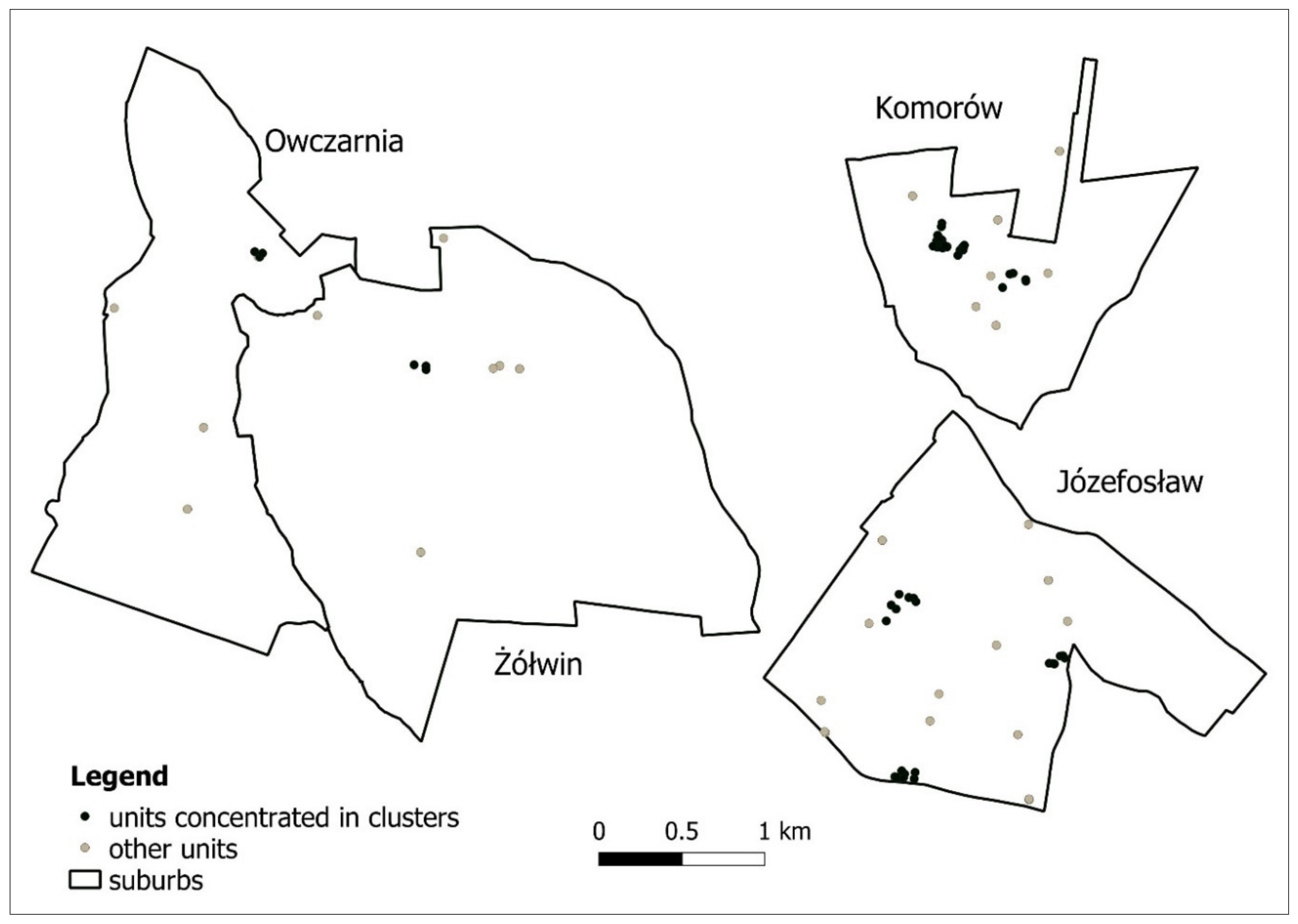
Figure 3.
Units of other than residential function concentrated in clusters.

Figure 4.
Open space area.

Table 1.
Dimensions of suburban spatial chaos, databases and functions used for calculating particular indicators.
Table 1.
Dimensions of suburban spatial chaos, databases and functions used for calculating particular indicators.
| Dimension of Spatial Chaos | Indicator of Spatial Chaos | Justification | Databases | Selected Layers. Functions and Methods of QGIS | |||
|---|---|---|---|---|---|---|---|
| Layers of Topographic Database | OSM | Google Maps and Street View | |||||
| 1. Street connectivity | spatial density of the public road network (main, collector and other) (m/1 km2) | spatial density of road network seems to be better indicator than demographic density because the latter is more dependent on the population density (population density does not affect walkability as much as the street density) | communication network, level3, administrative division units | - | data completion and verification | Layers: roads, division units. Line in polygon, Line intersections, Selection, Count points in polygon. | |
| the ratio of the number of four- or three-way intersections to the number of cul-de-sacs8 | large share of private cul-de-sacs is characteristic of Polish suburbs; cul-de-sacs decidedly limit the number of alternative walking routes | ||||||
| 2. Pedestrian infrastructure | the length of public roads equipped with a pavement9 in relation to the total length of three categories of roads: main, collector, and other (%) | pavements are basic element of pedestrian infrastructure encouraging suburbanites to walk, they are more important than street furniture and convenient pedestrian crossings | communication network | layer roads | data completion and verification | Layers: pavement roads, roads. Length. | |
| pedestrian design scale (indicator developed on the basis of the scale proposed by Replogle [54]): 0. no sidewalks, no safe roadsides and car restraints on most main and collective roads, or high proportion of dirt roads 1. no sidewalks, but safe roadsides and car restraints on most main and collective roads 2. sidewalks along selected main streets, in the case of most other roads, no safe roadsides and car restraints, or high proportion of dirt roads 3. sidewalks along selected main streets, in the case of most other roads, safe roadsides and car restraints 4. sidewalks along all main and some collector streets, no car restraints on most main and collective roads 5. sidewalks along all main and some collector streets, car restraints on most main and collective roads | pedestrian safety and comfort are important encouragement to walk, it is ensured by sidewalks, and in the case of their absence, by wide paved roadsides and car restraints, like speed bumps; width of pavements have been removed from the scale, because most pavements in Polish suburbs are relatively new, keep standards, and have a similar width | Not applicable | Not applicable | Not applicable | Not applicable | ||
| 3. Centrality/nuclearity on a local level | the ratio of units of other than residential function10 concentrated in clusters11 to the total number of such units (%) | concentration of various functions (other than residential) in a small area enhances using them all and by this improves profitability of retail and service points; it also animates social life | buildings | points layer | data completion | Layers: units, division units. DBSCAN clustering, Distance Matrix. | |
| average straight-line distance between all units of other than residential function (m) | close distances between individual units of different functions encourage people to walk and to explore the whole area of residence | ||||||
| 4. Proximity to public objects and services | straight-line distance from the centre of gravity12 of the suburb to the nearest public objects: primary school, church, bus stop/train station (m) | primary school, church, and bus stop/train station represent functions that are regularly used by all residents or specific age groups, and thus enable building social relations; when located within a suburb, they organize the whole space and flows of people | buildings | points layer | walking distance tool | Layers: centre, public points, buildings. Mean coordinates, Distance Matrix, Measure Line. | |
| the longest walking distance among all walking distances between a house located in the suburb and a nearest grocery13 (m) | objects used every day or very often should be as close as possible to the place of residence, preferably the distance should not exceed 300–500 m [60] | ||||||
| 5. Location of main public open space14 | the scale of location of the main local park (indicator developed on the basis of the scale proposed by Mantey [73]): 0. no local park within an administrative border of the suburb 1. space located somewhere “off the beaten track,” not visible from the nearest houses 2. space within a housing area, at some distance from nodes of activity15 (at least 500 m of walking distance), deprived of a safe pedestrian access 3. space within a housing area, at some distance from nodes of activity (at least 500 m of walking distance), but with a safe pedestrian access 4. space adjacent to a minor node of activity 5. space adjacent to the main node of activity | in Poland, municipalities have to pay high compensation if they want to purchase land for public space from private owners, this leads to the lack of local parks or their poor (random) location; as a result, the whole suburb is fragmented and the public space used not so frequently as it could be if its location is near the node of activity and the flow of pedestrians [81]. | Not applicable | Not applicable | Not applicable | Not applicable | |
| public open space area per 1000 residents in relation to the standard value of 2.83 ha/1000 people (%) (standard value according to Thompson [75]) | in the absence of urban standards in Poland, it will be possible to estimate how much the situation in individual suburbs differs from British standards | land use complexes | points layer, natural layer | data completion and verification | Layer: public space. Digitization of additional areas, Field calculator. | ||
Table 2.
The level of variability and weighting factors assigned to individual indicators.
| Coefficient of Variation (%) | |||||||||
| 29.3 | 111.1 | 80.2 | 40.0 | 30.9 | 34.0 | 30.0 | 44.8 | 53.8 | 64.9 |
| Weighting Factors | |||||||||
| 0.081 | 0.077 | 0.126 | 0.103 | 0.093 | 0.079 | 0.163 | 0.113 | 0.087 | 0.078 |
Table 3.
Results obtained for individual suburbs.
| Komorów | Józefosław | Owczarnia | Żółwin | ||
|---|---|---|---|---|---|
| Original values | |||||
| d | 13,968 | 7228 | 9265 | 7188 | |
| d | 13.09 | 1.9 | 1.32 | 1.61 | |
| d | 57 | 48 | 6 | 6 | |
| d | 5 | 4 | 2 | 2 | |
| d | 84 | 60 | 57 | 33 | |
| s | 303 | 853 | 917 | 749 | |
| s | 322 | 310 | 603 | 568 | |
| s | 830 | 1320 | 2900 | 2550 | |
| d | 5 | 3 | 2 | 1 | |
| d | 1.34 | 0.33 | 0.42 | 0.44 | |
| Synthetic Indicators of Spatial Chaos | |||||
| −1.445 | −0.069 | 0.693 | 0.821 | ||
| 0.000 | 0.056 | 0.089 | 0.093 | ||
| 0.001 | 0.047 | 0.090 | 0.093 | ||
s—stimulant; d—destimulant.
© 2020 by the authors. Licensee MDPI, Basel, Switzerland. This article is an open access article distributed under the terms and conditions of the Creative Commons Attribution (CC BY) license (http://creativecommons.org/licenses/by/4.0/).
Share and Cite
MDPI and ACS Style
Mantey, D.; Pokojski, W. New Indicators of Spatial Chaos in the Context of the Need for Retrofitting Suburbs. Land 2020, 9, 276. https://doi.org/10.3390/land9080276
AMA Style
Mantey D, Pokojski W. New Indicators of Spatial Chaos in the Context of the Need for Retrofitting Suburbs. Land. 2020; 9(8):276. https://doi.org/10.3390/land9080276
Chicago/Turabian StyleMantey, Dorota, and Wojciech Pokojski. 2020. "New Indicators of Spatial Chaos in the Context of the Need for Retrofitting Suburbs" Land 9, no. 8: 276. https://doi.org/10.3390/land9080276
Note that from the first issue of 2016, this journal uses article numbers instead of page numbers. See further details here.