Structural Variations in the Composition of Land Funds at Regional Scales across Russia


Abstract
1. Introduction
- District—A type of supraregional administrative division of Russia, which includes several territories based on a geographical principle (currently, eight federal districts exist).
- Land distribution—how lands of particular categories are spread out in a country, district, or territory.
- Land fund—the total of available land resources in a country, district, or territory.
- Land fund composition—a division of a land fund into land categories.
- Land use—the total of arrangements, activities, and inputs that people undertake in a certain land cover type.
- Territory—an umbrella term to designate various types of administrative divisions of the Russian Federation (oblasts, krais, republics, autonomous districts, and autonomous republics).
2. Materials and Methods
2.1. Stage 1: Land Categories
2.2. Stage 2: Composition of Land Funds
2.3. Stage 3: Agricultural Land Activity
2.4. Stage 4: Revealing Structural Variations of Agricultural and Non-Agricultural Land Categories
2.5. Stage 5: Significance of Correlations
2.6. Territories and Data
3. Results
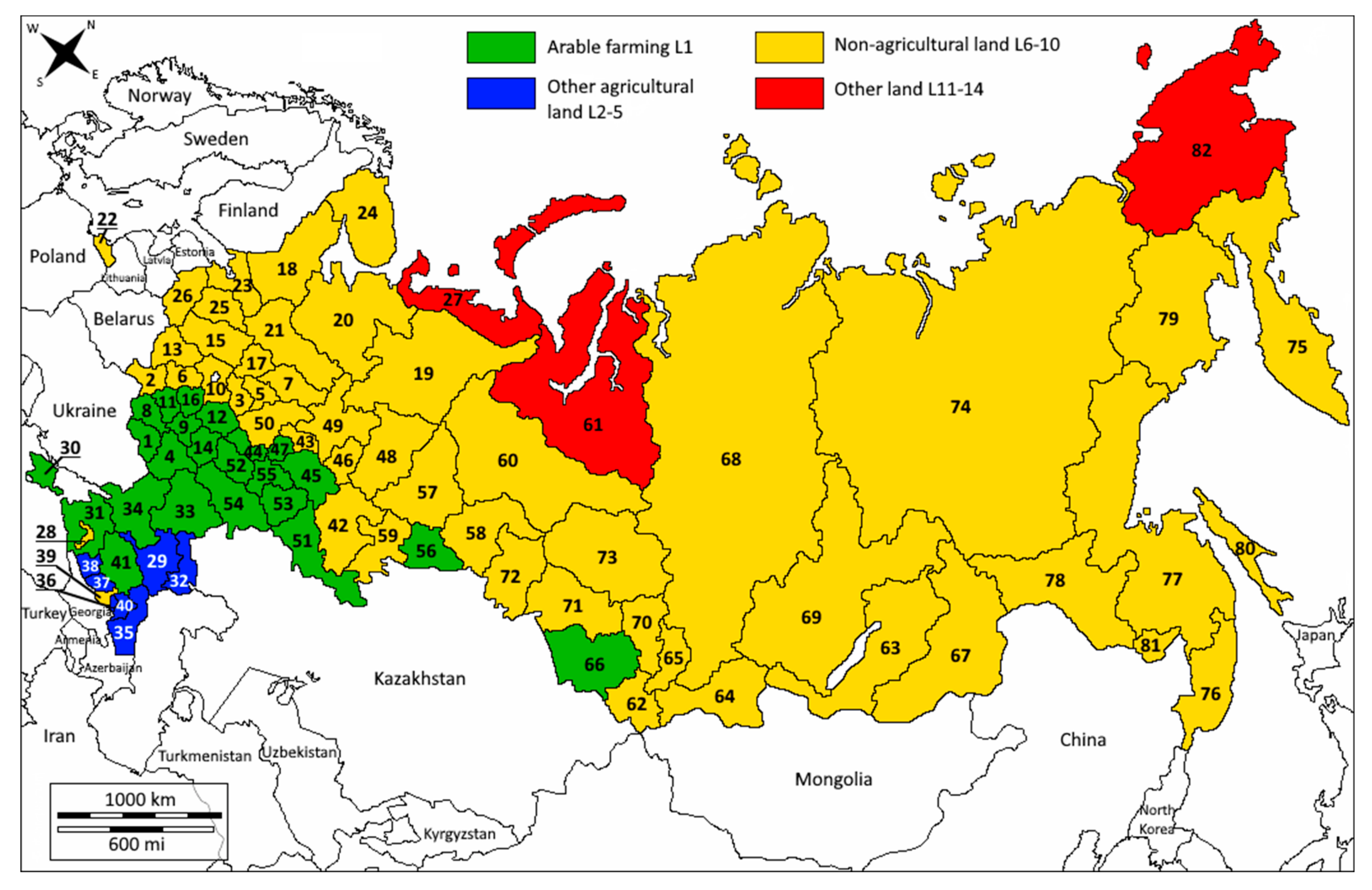
3.1. Composition of Land Funds
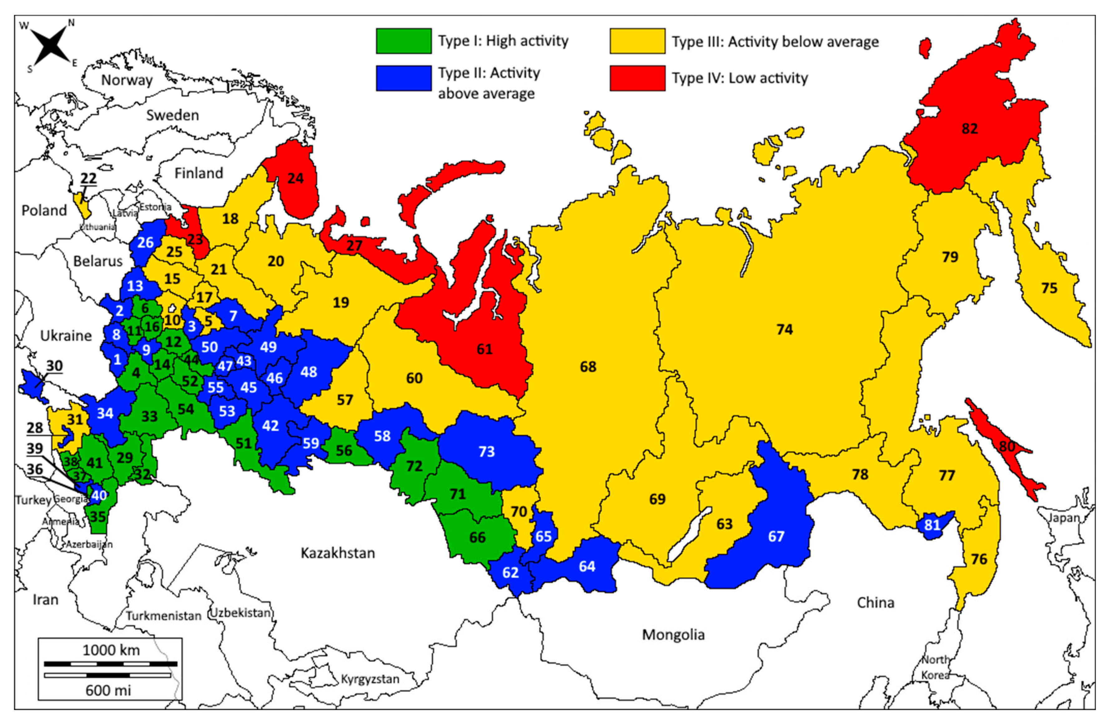
3.2. Agricultural Land Activity
3.3. Correlation Analysis
4. Discussion
5. Conclusions
Author Contributions
Funding
Conflicts of Interest
Appendix A

| Territory | Total | L1 | L2 | L3 | L4 | L5 | L6 | L7 | L8 | L9 | L10 | L11 | L12 | L13 |
|---|---|---|---|---|---|---|---|---|---|---|---|---|---|---|
| T1 | 2713.4 | 1645.2 | 0 | 34.0 | 55.8 | 399.3 | 241.9 | 90.5 | 25.1 | 73.1 | 57.9 | 22.5 | 6.5 | 61.6 |
| T2 | 3485.7 | 1174.9 | 121.4 | 26.0 | 205.5 | 346.5 | 1183.6 | 121.4 | 31.6 | 56.8 | 72.0 | 75.1 | 5.1 | 65.8 |
| T3 | 2908.4 | 605.7 | 46.6 | 20.0 | 163.9 | 159.1 | 1582.7 | 74.9 | 32.7 | 38.0 | 75.0 | 38.3 | 16.3 | 55.2 |
| T4 | 5221.6 | 3046.2 | 41.9 | 52.8 | 159.0 | 776.8 | 482.4 | 149.5 | 64.0 | 113.4 | 121.1 | 40.6 | 1.9 | 172.0 |
| T5 | 2143.7 | 565.9 | 9.8 | 9.0 | 124.1 | 112.5 | 1047.8 | 28.5 | 65.0 | 42.0 | 51.2 | 50.3 | 7.4 | 30.2 |
| T6 | 2977.7 | 956.1 | 36.1 | 21.0 | 131.2 | 232.2 | 1376.9 | 35.5 | 21.0 | 56.9 | 50.2 | 28.6 | 2.1 | 29.9 |
| T7 | 6021.1 | 655.0 | 31.2 | 5.6 | 154.5 | 148.3 | 4574.1 | 98.9 | 97.0 | 35.6 | 101.7 | 86.8 | 5.7 | 26.7 |
| T8 | 2999.7 | 1943.4 | 0.7 | 27.9 | 101.6 | 364.3 | 249.3 | 68.1 | 38.3 | 56.4 | 72.5 | 32.1 | 11.0 | 34.1 |
| T9 | 2404.7 | 1553.9 | 0.1 | 35.2 | 83.6 | 281.0 | 190.7 | 61.4 | 27.0 | 47.9 | 61.7 | 16.4 | 2.5 | 43.3 |
| T10 | 4579.9 | 1130.3 | 6.7 | 113.9 | 183.0 | 229.4 | 1998.3 | 35.2 | 90.1 | 303.1 | 158.8 | 50.6 | 34.7 | 98.8 |
| T11 | 2465.2 | 1570.0 | 55.7 | 25.3 | 58.6 | 341.5 | 203.1 | 74.2 | 14.4 | 21.9 | 72.8 | 3.8 | 0.7 | 23.2 |
| T12 | 3960.5 | 1535.2 | 26.1 | 24.6 | 202.6 | 722.4 | 1067.8 | 66.3 | 67.2 | 37.1 | 105.1 | 55.4 | 6.6 | 44.1 |
| T13 | 4977.9 | 1461.7 | 17.7 | 19.5 | 215.1 | 380.0 | 2167.6 | 357.6 | 53.7 | 55.7 | 86.5 | 115.3 | 18.0 | 29.5 |
| T14 | 3446.2 | 2127.5 | 9.6 | 32.4 | 166.0 | 388.8 | 371.7 | 97.9 | 42.8 | 55.1 | 60.8 | 43.9 | 1.7 | 48.0 |
| T15 | 8420.1 | 1504.3 | 19.4 | 14.7 | 379.1 | 501.0 | 4742.2 | 233.3 | 248.1 | 96.9 | 116.4 | 465.2 | 20.3 | 79.2 |
| T16 | 2567.9 | 1554.4 | 7.6 | 45.0 | 67.9 | 298.0 | 372.3 | 43.0 | 22.8 | 32.3 | 90.4 | 1.9 | 10.0 | 22.3 |
| T17 | 3617.7 | 793.3 | 0.3 | 14.6 | 123.7 | 196.1 | 1725.7 | 93.0 | 386.8 | 59.4 | 65.8 | 109.7 | 15.2 | 34.1 |
| Territory | Total | L1 | L2 | L3 | L4 | L5 | L6 | L7 | L8 | L9 | L10 | L11 | L12 | L13 |
|---|---|---|---|---|---|---|---|---|---|---|---|---|---|---|
| T18 | 18,052.0 | 82.3 | 0.1 | 5.9 | 85.4 | 39.2 | 9850.2 | 22.1 | 4188.2 | 38.3 | 87.6 | 3543.6 | 13.4 | 95.7 |
| T19 | 41,677.4 | 102.4 | 0 | 6.5 | 239.6 | 69.6 | 31,093.5 | 135.6 | 641.5 | 48.2 | 144.8 | 4073.1 | 15.8 | 5106.8 |
| T20 | 41,310.3 | 302.5 | 1.8 | 9.1 | 304.1 | 109.8 | 22,948.6 | 126.3 | 811.5 | 93.3 | 131.3 | 5823.3 | 5.5 | 10,643.2 |
| T21 | 14,452.7 | 822.0 | 48.0 | 9.4 | 343.9 | 225.2 | 10,456.4 | 330.9 | 658.6 | 38.3 | 178.3 | 1271.8 | 22.2 | 47.7 |
| T22 | 1512.5 | 392.6 | 0 | 14.3 | 153.6 | 248.9 | 295.1 | 18.8 | 200.3 | 40.6 | 40.9 | 31.0 | 4.4 | 72.0 |
| T23 | 8390.8 | 434.1 | 0 | 44.4 | 194.6 | 125.4 | 5015.7 | 125.3 | 1266.8 | 58.7 | 112.7 | 830.0 | 23.0 | 160.1 |
| T24 | 14,490.2 | 19.4 | 0 | 3.1 | 2.8 | 0.3 | 5383.6 | 580.8 | 1191.5 | 37.1 | 31.3 | 5701.2 | 19.7 | 1519.4 |
| T25 | 5450.1 | 510.6 | 4.2 | 6.1 | 173.1 | 135.9 | 3580.9 | 138.6 | 174.8 | 25.5 | 69.8 | 548.5 | 10.4 | 71.7 |
| T26 | 5539.9 | 744.3 | 186.4 | 20.5 | 279.0 | 280.9 | 2249.0 | 785.3 | 375.3 | 34.8 | 71.9 | 476.2 | 8.9 | 27.4 |
| T27 | 17,681.0 | 0.2 | 0 | 0 | 19.8 | 5.7 | 1740.8 | 1439.2 | 1000.5 | 12.8 | 10.8 | 3381.8 | 2.5 | 10,066.9 |
| Territory | Total | L1 | L2 | L3 | L4 | L5 | L6 | L7 | L8 | L9 | L10 | L11 | L12 | L13 |
|---|---|---|---|---|---|---|---|---|---|---|---|---|---|---|
| T28 | 779.2 | 259.6 | 0.3 | 9.3 | 4.9 | 85.7 | 288.8 | 7.7 | 53.5 | 22.1 | 18.8 | 4.0 | 0.3 | 24.2 |
| T29 | 7473.1 | 836.9 | 10.6 | 2.5 | 103.2 | 5363.6 | 32.6 | 42.3 | 175.6 | 32.2 | 65.1 | 123.5 | 4.0 | 681.0 |
| T30 | 2608.1 | 1271.6 | 10.6 | 75.8 | 1.9 | 433.6 | 266.2 | 35.0 | 211.7 | 118.8 | 43.4 | 5.2 | 1.5 | 132.8 |
| T31 | 7548.5 | 3985.4 | 0.2 | 125.2 | 63.1 | 531.1 | 1541.3 | 158.7 | 385.6 | 202.9 | 196.0 | 179.6 | 5.4 | 174.0 |
| T32 | 4902.4 | 352.0 | 6.7 | 9.8 | 404.8 | 2482.7 | 104.2 | 19.5 | 684.6 | 28.2 | 57.4 | 114.7 | 0.5 | 637.3 |
| T33 | 11,287.7 | 5854.0 | 4.7 | 42.8 | 206.9 | 2652.8 | 591.0 | 131.3 | 489.8 | 165.9 | 117.6 | 35.2 | 3.0 | 992.7 |
| T34 | 10,096.7 | 5907.3 | 0 | 58.2 | 88.4 | 2459.2 | 293.0 | 281.9 | 346.1 | 150.8 | 220.5 | 55.0 | 7.1 | 229.2 |
| Territory | Total | L1 | L2 | L3 | L4 | L5 | L6 | L7 | L8 | L9 | L10 | L11 | L12 | L13 |
|---|---|---|---|---|---|---|---|---|---|---|---|---|---|---|
| T35 | 5027.0 | 520.1 | 4.8 | 72.4 | 162.3 | 2588.6 | 585.0 | 57.2 | 176.9 | 34.5 | 63.0 | 20.6 | 2.5 | 739.1 |
| T36 | 362.8 | 111.0 | 0 | 4.7 | 9.7 | 96.6 | 101.0 | 2.3 | 1.7 | 4.5 | 5.5 | 0.1 | 0.1 | 25.6 |
| T37 | 1247.0 | 300.7 | 0 | 30.1 | 56.3 | 309.3 | 196.8 | 13.3 | 15.5 | 17.6 | 26.8 | 1.2 | 1.0 | 278.4 |
| T38 | 1427.7 | 161.1 | 3.8 | 4.9 | 140.9 | 353.2 | 431.2 | 9.7 | 22.5 | 13.9 | 14.1 | 1.3 | 0.8 | 270.3 |
| T39 | 798.7 | 202.4 | 0.4 | 5.1 | 23.2 | 169.7 | 205.9 | 9.7 | 11.5 | 19.1 | 12.0 | 0.5 | 0.3 | 138.9 |
| T40 | 1564.7 | 332.2 | 0.2 | 11.0 | 56.8 | 575.2 | 336.0 | 27.6 | 28.6 | 43.4 | 21.5 | 2.7 | 1.4 | 128.1 |
| T41 | 6616.0 | 3998.6 | 14.0 | 44.2 | 104.9 | 1625.8 | 110.2 | 144.1 | 127.0 | 107.5 | 147.9 | 28.8 | 3.4 | 159.6 |
| Territory | Total | L1 | L2 | L3 | L4 | L5 | L6 | L7 | L8 | L9 | L10 | L11 | L12 | L13 |
|---|---|---|---|---|---|---|---|---|---|---|---|---|---|---|
| T42 | 14,294.7 | 3670.5 | 0 | 43.6 | 1266.7 | 2346.1 | 5765.6 | 227.9 | 149.9 | 132.1 | 260.1 | 50.8 | 17.2 | 364.2 |
| T43 | 2337.5 | 472.1 | 128.0 | 7.9 | 56.6 | 108.2 | 1340.6 | 18.9 | 85.0 | 26.2 | 39.5 | 33.1 | 1.4 | 20.0 |
| T44 | 2612.8 | 1084.8 | 56.8 | 14.5 | 62.3 | 437.2 | 726.1 | 64.8 | 20.8 | 33.5 | 53.0 | 15.9 | 1.5 | 41.6 |
| T45 | 6784.7 | 3420.6 | 0.7 | 41.1 | 144.2 | 932.8 | 1199.1 | 129.4 | 451.6 | 141.7 | 157.8 | 50.6 | 4.8 | 110.3 |
| T46 | 4206.1 | 1382.3 | 9.3 | 15.2 | 112.5 | 321.5 | 2019.1 | 102.0 | 53.8 | 36.2 | 99.5 | 16.7 | 5.3 | 32.7 |
| T47 | 1834.3 | 806.3 | 6.2 | 19.9 | 48.3 | 153.8 | 603.6 | 17.5 | 48.1 | 35.3 | 60.1 | 5.1 | 0.5 | 29.6 |
| T48 | 16,023.6 | 1980.7 | 67.8 | 25.4 | 388.8 | 376.5 | 11,749.2 | 145.5 | 399.6 | 124.1 | 209.1 | 369.8 | 8.5 | 178.6 |
| T49 | 12,037.4 | 2480.3 | 51.8 | 15.0 | 374.2 | 399.1 | 7949.0 | 150.6 | 118.0 | 48.7 | 148.4 | 133.3 | 12.9 | 156.1 |
| T50 | 7662.4 | 2035.8 | 180.0 | 33.8 | 218.6 | 642.5 | 3817.1 | 90.2 | 162.7 | 112.8 | 143.4 | 123.0 | 6.0 | 96.5 |
| T51 | 12,370.2 | 6115.3 | 0 | 23.0 | 698.0 | 3979.5 | 618.6 | 199.3 | 111.3 | 158.7 | 184.7 | 15.3 | 13.0 | 253.5 |
| T52 | 4335.2 | 2263.6 | 153.4 | 22.5 | 71.4 | 528.1 | 975.7 | 77.2 | 42.2 | 59.7 | 89.7 | 13.5 | 0.9 | 37.3 |
| T53 | 5356.5 | 2937.5 | 103.5 | 42.3 | 67.0 | 847.5 | 685.6 | 104.5 | 226.0 | 103.0 | 123.7 | 42.0 | 3.9 | 70.0 |
| T54 | 10,124.0 | 5981.1 | 0 | 39.9 | 122.2 | 2400.5 | 614.2 | 121.2 | 357.9 | 113.3 | 149.4 | 19.2 | 2.4 | 202.7 |
| T55 | 3718.1 | 1655.7 | 105.8 | 17.7 | 37.8 | 390.3 | 1035.2 | 55.0 | 228.5 | 34.8 | 85.6 | 10.7 | 1.4 | 59.6 |
| Territory | Total | L1 | L2 | L3 | L4 | L5 | L6 | L7 | L8 | L9 | L10 | L11 | L12 | L13 |
|---|---|---|---|---|---|---|---|---|---|---|---|---|---|---|
| T56 | 7148.8 | 2402.6 | 459.3 | 12.4 | 559.0 | 1024.8 | 1759.5 | 37.2 | 318.7 | 49.1 | 86.3 | 383.9 | 1.1 | 54.9 |
| T57 | 19,430.7 | 1470.4 | 99.5 | 32.4 | 624.3 | 351.1 | 13,631.8 | 230.7 | 262.3 | 162.4 | 228.5 | 2046.2 | 61.8 | 229.3 |
| T58 | 16,012.2 | 1353.0 | 364.7 | 11.7 | 895.8 | 756.7 | 7112.8 | 144.9 | 508.5 | 80.0 | 96.1 | 4609.1 | 4.6 | 74.3 |
| T59 | 8852.9 | 3058.8 | 55.0 | 38.3 | 591.1 | 1352.0 | 2707.3 | 75.2 | 275.9 | 137.8 | 145.5 | 192.7 | 31.8 | 191.5 |
| T60 | 53,480.1 | 13.1 | 3.0 | 10.5 | 343.8 | 259.7 | 28,693.6 | 156.5 | 3185.4 | 141.6 | 170.7 | 19,913.4 | 55.7 | 533.1 |
| T61 | 76,925.0 | 0.9 | 0 | 0.2 | 165.3 | 57.3 | 18,763.5 | 4380.3 | 13,319.9 | 120.5 | 170.7 | 14,798.8 | 103.7 | 25,043.9 |
| Territory | Total | L1 | L2 | L3 | L4 | L5 | L6 | L7 | L8 | L9 | L10 | L11 | L12 | L13 |
|---|---|---|---|---|---|---|---|---|---|---|---|---|---|---|
| T62 | 9290.3 | 143.5 | 2.2 | 1.7 | 120.9 | 1522.8 | 4357.7 | 190.0 | 86.3 | 10.9 | 23.1 | 73.3 | 0.4 | 2757.5 |
| T63 | 35,133.4 | 829.6 | 61.6 | 8.2 | 389.6 | 1856.8 | 23,660.6 | 220.7 | 2409.0 | 73.2 | 86.3 | 487.3 | 7.8 | 5042.7 |
| T64 | 16,860.4 | 191.3 | 147.9 | 0.9 | 76.5 | 3416.6 | 8667.2 | 450.1 | 228.1 | 21.7 | 29.3 | 1026.4 | 5.5 | 2598.9 |
| T65 | 6156.9 | 685.0 | 40.0 | 7.3 | 160.4 | 1022.5 | 3288.9 | 23.1 | 112.2 | 30.0 | 39.3 | 32.1 | 12.7 | 703.4 |
| T66 | 16,799.6 | 6654.4 | 298.9 | 27.8 | 1235.6 | 2789.7 | 4029.3 | 205.8 | 442.6 | 131.9 | 195.5 | 374.7 | 3.6 | 409.8 |
| T67 | 43,189.2 | 484.1 | 951.5 | 5.7 | 1722.6 | 4481.7 | 30,782.9 | 497.5 | 318.7 | 152.1 | 114.3 | 1076.9 | 24.2 | 2577.0 |
| T68 | 236,679.7 | 3120.1 | 136.4 | 37.4 | 781.8 | 1334.1 | 120,936.8 | 3185.0 | 9221.5 | 175.3 | 182.5 | 22,690.2 | 17.3 | 74,861.3 |
| T69 | 77,484.6 | 1734.5 | 3.3 | 30.0 | 390.1 | 640.8 | 66,080.5 | 235.1 | 2639.0 | 165.1 | 260.9 | 1709.4 | 26.3 | 3569.6 |
| T70 | 9572.5 | 1539.4 | 0.1 | 27.1 | 471.3 | 582.5 | 6074.7 | 163.2 | 91.7 | 107.5 | 174.5 | 90.5 | 83.4 | 166.6 |
| T71 | 17,775.6 | 3772.1 | 81.0 | 33.6 | 2197.9 | 2315.0 | 4799.2 | 280.3 | 766.5 | 102.4 | 166.8 | 3059.6 | 1.7 | 199.5 |
| T72 | 14,114.0 | 4156.6 | 175.9 | 26.5 | 1096.2 | 1265.5 | 4667.7 | 89.4 | 289.8 | 93.9 | 150.7 | 2026.8 | 5.0 | 70.0 |
| T73 | 31,439.1 | 675.9 | 1.3 | 9.4 | 479.9 | 204.5 | 19,939.9 | 88.1 | 608.3 | 42.5 | 87.9 | 9173.9 | 7.1 | 120.4 |
| Territory | Total | L1 | L2 | L3 | L4 | L5 | L6 | L7 | L8 | L9 | L10 | L11 | L12 | L13 |
|---|---|---|---|---|---|---|---|---|---|---|---|---|---|---|
| T74 | 308,352.3 | 105.3 | 19.0 | 1.0 | 719.5 | 795.4 | 164,862.0 | 1837.7 | 13,087.5 | 82.6 | 129.1 | 19,783.6 | 30.9 | 106,898.7 |
| T75 | 46,427.5 | 64.3 | 1.0 | 5.3 | 97.3 | 307.7 | 26,810.0 | 305.8 | 844.5 | 16.3 | 17.0 | 2523.3 | 2.9 | 15,432.1 |
| T76 | 16,467.3 | 755.0 | 60.8 | 25.9 | 361.8 | 445.9 | 13,023.3 | 407.6 | 424.6 | 111.1 | 101.3 | 466.9 | 16.8 | 266.3 |
| T77 | 78,763.3 | 98.4 | 25.1 | 16.8 | 401.9 | 123.4 | 59,571.6 | 231.8 | 1476.3 | 79.3 | 95.7 | 5605.9 | 6.1 | 11,031.0 |
| T78 | 36,190.8 | 1577.2 | 244.0 | 11.9 | 418.0 | 482.5 | 26,136.8 | 268.4 | 1151.0 | 54.1 | 136.3 | 4794.1 | 12.7 | 903.8 |
| T79 | 46,246.4 | 23.8 | 3.5 | 0.1 | 51.5 | 42.6 | 28,467.1 | 340.8 | 477.3 | 9.5 | 14.5 | 4815.4 | 77.4 | 11,922.9 |
| T80 | 8710.1 | 51.2 | 0 | 7.6 | 63.6 | 60.0 | 6607.9 | 347.5 | 233.2 | 34.0 | 33.1 | 642.0 | 10.5 | 619.5 |
| T81 | 3627.1 | 94.6 | 70.3 | 3.1 | 119.2 | 250.0 | 1783.2 | 139.1 | 35.3 | 12.1 | 20.7 | 914.5 | 1.5 | 183.5 |
| T82 | 72,148.1 | 0.1 | 0 | 0 | 8.2 | 0.3 | 13,015.1 | 3878.3 | 2442.7 | 4.5 | 22.2 | 2833.0 | 47.5 | 49,896.2 |
Appendix B
| Parameter | T1 | T2 | T3 | T4 | T5 | T6 | T7 | T8 | T9 | T10 | T11 | T12 | T13 | T14 | T15 | T16 | T17 | |
|---|---|---|---|---|---|---|---|---|---|---|---|---|---|---|---|---|---|---|
| L1 | 0.606 | 0.337 | 0.208 | 0.583 | 0.264 | 0.321 | 0.109 | 0.648 | 0.646 | 0.255 | 0.637 | 0.388 | 0.294 | 0.617 | 0.179 | 0.605 | 0.219 | 0.367 |
| VL1 | −0.002 | +0.006 | - | −0.003 | −0.003 | - | −0.002 | −0.001 | - | −0.008 | - | - | - | −0.001 | - | −0.001 | - | |
| L2 | 0 | 0.035 | 0.016 | 0.008 | 0.005 | 0.012 | 0.005 | 0 | 0 | 0.002 | 0.023 | 0.007 | 0.004 | 0.003 | 0.002 | 0.003 | 0 | 0.007 |
| VL2 | - | −0.007 | - | - | +0.001 | - | - | - | - | +0.002 | - | - | - | −0.002 | - | - | - | |
| L3 | 0.013 | 0.007 | 0.007 | 0.010 | 0.004 | 0.007 | 0.001 | 0.009 | 0.015 | 0.026 | 0.010 | 0.006 | 0.004 | 0.009 | 0.002 | 0.018 | 0.004 | 0.008 |
| VL3 | - | - | - | - | - | - | - | - | - | +0.001 | - | - | - | - | - | - | - | |
| L4 | 0.021 | 0.059 | 0.056 | 0.030 | 0.058 | 0.044 | 0.026 | 0.034 | 0.035 | 0.041 | 0.024 | 0.051 | 0.043 | 0.048 | 0.045 | 0.026 | 0.034 | 0.040 |
| VL4 | - | +0.001 | - | - | - | - | - | - | - | −0.001 | - | - | - | +0.006 | - | −0.001 | −0 | |
| L5 | 0.147 | 0.099 | 0.055 | 0.149 | 0.052 | 0.078 | 0.025 | 0.121 | 0.117 | 0.052 | 0.139 | 0.182 | 0.076 | 0.113 | 0.060 | 0.116 | 0.054 | 0.090 |
| VL5 | - | - | - | +0.002 | - | - | - | - | - | −0.003 | - | - | - | +0.010 | - | −0.001 | - | |
| L6 | 0.089 | 0.340 | 0.544 | 0.092 | 0.489 | 0.462 | 0.760 | 0.083 | 0.079 | 0.451 | 0.082 | 0.270 | 0.435 | 0.108 | 0.563 | 0.145 | 0.477 | 0.363 |
| VL6 | - | - | - | +0.006 | - | - | - | - | - | +0.001 | - | +0.001 | - | - | +0.002 | - | +0.001 | |
| L7 | 0.033 | 0.035 | 0.026 | 0.029 | 0.013 | 0.012 | 0.016 | 0.023 | 0.026 | 0.008 | 0.030 | 0.017 | 0.072 | 0.028 | 0.028 | 0.017 | 0.026 | 0.027 |
| VL7 | - | - | - | −0.006 | - | - | +0.002 | - | - | −0.001 | - | - | −0.001 | +0.006 | −0.002 | - | - | |
| L8 | 0.009 | 0.009 | 0.011 | 0.012 | 0.030 | 0.007 | 0.016 | 0.013 | 0.011 | 0.020 | 0.006 | 0.017 | 0.011 | 0.012 | 0.029 | 0.009 | 0.107 | 0.020 |
| VL8 | - | - | - | - | - | - | - | - | - | - | - | - | - | - | - | - | - | |
| L9 | 0.027 | 0.016 | 0.013 | 0.022 | 0.020 | 0.019 | 0.006 | 0.019 | 0.020 | 0.068 | 0.009 | 0.009 | 0.011 | 0.016 | 0.012 | 0.013 | 0.016 | 0.019 |
| VL9 | +0.001 | - | - | +0.001 | +0.001 | - | - | +0.001 | - | +0.005 | - | - | - | - | - | +0.003 | +0.001 | |
| L10 | 0.021 | 0.021 | 0.026 | 0.023 | 0.024 | 0.017 | 0.017 | 0.024 | 0.026 | 0.036 | 0.030 | 0.027 | 0.017 | 0.018 | 0.014 | 0.035 | 0.018 | 0.022 |
| VL10 | +0.001 | - | - | - | - | - | - | - | - | - | - | - | - | - | - | - | - | |
| L11 | 0.008 | 0.022 | 0.013 | 0.008 | 0.023 | 0.010 | 0.014 | 0.011 | 0.007 | 0.011 | 0.002 | 0.014 | 0.023 | 0.013 | 0.065 | 0.001 | 0.030 | 0.019 |
| VL11 | - | - | - | - | - | - | - | - | - | - | - | - | - | - | - | - | - | |
| L12 | 0.002 | 0.001 | 0.006 | 0 | 0.003 | 0.001 | 0.001 | 0.004 | 0.001 | 0.008 | 0 | 0.002 | 0.004 | 0 | 0.002 | 0.004 | 0.004 | 0.003 |
| VL12 | - | - | - | - | - | - | - | - | - | - | - | - | - | - | - | - | - | |
| L13 | 0.023 | 0.019 | 0.018 | 0.033 | 0.014 | 0.010 | 0.004 | 0.011 | 0.018 | 0.022 | 0.010 | 0.011 | 0.006 | 0.013 | 0.009 | 0.009 | 0.009 | 0.015 |
| VL13 | - | −0.005 | −0.006 | −0.007 | −0.003 | −0.001 | −0.002 | −0.004 | −0.004 | −0.003 | −0.005 | −0.005 | −0.002 | −0.004 | −0.001 | −0.003 | −0.004 |
| Parameter | T18 | T19 | T20 | T21 | T22 | T23 | T24 | T25 | T26 | T27 | |
|---|---|---|---|---|---|---|---|---|---|---|---|
| L1 | 0.005 | 0.002 | 0.007 | 0.057 | 0.260 | 0.052 | 0.001 | 0.094 | 0.134 | 0 | 0.020 |
| VL1 | - | - | - | +0.004 | −0.005 | +0.002 | - | −0.002 | +0.003 | - | |
| L2 | 0 | 0 | 0 | 0.003 | 0 | 0 | 0 | 0.001 | 0.034 | 0 | 0.001 |
| VL2 | - | - | - | - | - | - | - | - | −0.003 | - | |
| L3 | 0 | 0 | 0 | 0.001 | 0.009 | 0.005 | 0 | 0.001 | 0.004 | 0 | 0.001 |
| VL3 | - | - | - | - | +0.001 | −0.001 | - | - | - | - | |
| L4 | 0.005 | 0.006 | 0.007 | 0.024 | 0.102 | 0.023 | 0 | 0.032 | 0.050 | 0.001 | 0.011 |
| VL4 | +0.001 | −0.001 | +0.001 | −0.003 | +0.004 | −0.002 | - | +0.001 | +0.003 | - | |
| L5 | 0.002 | 0.002 | 0.003 | 0.016 | 0.165 | 0.015 | 0 | 0.025 | 0.051 | 0 | 0.007 |
| VL5 | - | - | - | +0.002 | −0.005 | +0.001 | - | +0.001 | −0.003 | - | |
| L6 | 0.546 | 0.746 | 0.556 | 0.723 | 0.195 | 0.598 | 0.372 | 0.657 | 0.406 | 0.098 | 0.549 |
| VL6 | +0.012 | −0.009 | +0.004 | −0.033 | +0.017 | −0.005 | +0.023 | −0.008 | +0.014 | +0.002 | |
| L7 | 0.001 | 0.003 | 0.003 | 0.023 | 0.012 | 0.015 | 0.040 | 0.025 | 0.142 | 0.081 | 0.022 |
| VL7 | - | - | - | +0.002 | - | - | −0.001 | −0.001 | −0.011 | +0.002 | |
| L8 | 0.232 | 0.015 | 0.020 | 0.046 | 0.132 | 0.151 | 0.082 | 0.032 | 0.068 | 0.057 | 0.062 |
| VL8 | +0.006 | −0.001 | - | +0.002 | +0.004 | −0.003 | - | - | +0.001 | +0.002 | |
| L9 | 0.002 | 0.001 | 0.002 | 0.003 | 0.027 | 0.007 | 0.003 | 0.005 | 0.006 | 0.001 | 0.003 |
| VL9 | - | - | - | - | −0.003 | - | - | - | +0.001 | - | |
| L10 | 0.005 | 0.003 | 0.003 | 0.012 | 0.027 | 0.013 | 0.002 | 0.013 | 0.013 | 0.001 | 0.005 |
| VL10 | −0.001 | - | - | +0.001 | −0.002 | - | - | - | −0.001 | - | |
| L11 | 0.196 | 0.098 | 0.141 | 0.088 | 0.020 | 0.099 | 0.393 | 0.101 | 0.086 | 0.191 | 0.152 |
| VL11 | +0.004 | −0.003 | +0.010 | +0.003 | - | −0.002 | +0.007 | −0.013 | −0.002 | +0.004 | |
| L12 | 0.001 | 0 | 0 | 0.002 | 0.003 | 0.003 | 0.001 | 0.002 | 0.002 | 0 | 0.001 |
| VL12 | - | - | - | - | - | - | - | - | - | - | |
| L13 | 0.005 | 0.123 | 0.258 | 0.003 | 0.048 | 0.019 | 0.105 | 0.013 | 0.005 | 0.569 | 0.165 |
| VL13 | −0.004 | −0.023 | +0.011 | - | +0.014 | +0.008 | +0.025 | +0.005 | −0.004 | +0.054 |
| Parameter | T28 | T29 | T30 | T31 | T32 | T33 | T34 | |
|---|---|---|---|---|---|---|---|---|
| L1 | 0.333 | 0.112 | 0.488 | 0.528 | 0.072 | 0.519 | 0.585 | 0.413 |
| VL1 | −0.002 | −0.007 | - | −0.001 | +0.003 | −0.007 | +0.004 | |
| L2 | 0 | 0.001 | 0.004 | 0 | 0.001 | 0 | 0 | 0.001 |
| VL2 | - | - | +0.001 | - | - | - | - | |
| L3 | 0.012 | 0 | 0.029 | 0.017 | 0.002 | 0.004 | 0.006 | 0.007 |
| VL3 | +0.002 | - | −0.003 | +0.002 | - | - | +0.001 | |
| L4 | 0.006 | 0.014 | 0.001 | 0.008 | 0.083 | 0.018 | 0.009 | 0.020 |
| VL4 | - | −0.001 | - | - | +0.004 | +0.002 | −0.005 | |
| L5 | 0.110 | 0.718 | 0.166 | 0.070 | 0.506 | 0.235 | 0.244 | 0.313 |
| VL5 | −0.006 | +0.005 | −0.003 | −0.004 | −0.010 | +0.009 | +0.003 | |
| L6 | 0.371 | 0.004 | 0.102 | 0.204 | 0.021 | 0.052 | 0.029 | 0.070 |
| VL6 | +0.004 | - | −0.002 | +0.005 | −0.001 | −0.002 | −0.003 | |
| L7 | 0.010 | 0.006 | 0.013 | 0.021 | 0.004 | 0.012 | 0.028 | 0.015 |
| VL7 | - | - | +0.001 | −0.002 | - | - | +0.002 | |
| L8 | 0.069 | 0.023 | 0.081 | 0.051 | 0.140 | 0.043 | 0.034 | 0.052 |
| VL8 | −0.006 | +0.001 | −0.003 | +0.002 | −0.005 | - | - | |
| L9 | 0.028 | 0.004 | 0.046 | 0.027 | 0.006 | 0.015 | 0.015 | 0.016 |
| VL9 | +0.002 | - | −0.001 | +0.001 | - | - | +0.001 | |
| L10 | 0.024 | 0.009 | 0.017 | 0.026 | 0.012 | 0.010 | 0.022 | 0.016 |
| VL10 | −0.001 | - | +0..002 | - | - | - | −0.001 | |
| L11 | 0.005 | 0.017 | 0.002 | 0.024 | 0.023 | 0.003 | 0.005 | 0.012 |
| VL11 | - | +0.001 | - | - | +0.001 | - | - | |
| L12 | 0 | 0.001 | 0.001 | 0.001 | 0 | 0 | 0.001 | 0 |
| VL12 | - | - | - | - | - | - | - | |
| L13 | 0.031 | 0.091 | 0.051 | 0.023 | 0.130 | 0.088 | 0.023 | 0.064 |
| VL13 | +0.013 | +0.014 | - | +0.004 | +0.033 | +0.021 | +0.004 |
| Parameter | T35 | T36 | T37 | T38 | T39 | T40 | T41 | |
|---|---|---|---|---|---|---|---|---|
| L1 | 0.103 | 0.306 | 0.241 | 0.113 | 0.253 | 0.212 | 0.604 | 0.330 |
| VL1 | +0.002 | −0.003 | +0.006 | +0.002 | −0.003 | +0.004 | +0.011 | |
| L2 | 0.001 | 0 | 0 | 0.003 | 0.001 | 0 | 0.002 | 0.001 |
| VL2 | - | - | - | - | - | - | - | |
| L3 | 0.014 | 0.013 | 0.024 | 0.003 | 0.006 | 0.007 | 0.007 | 0.010 |
| VL3 | −0.001 | +0.002 | −0.005 | - | - | +0.001 | −0.001 | |
| L4 | 0.032 | 0.027 | 0.045 | 0.099 | 0.029 | 0.036 | 0.016 | 0.033 |
| VL4 | +0.003 | +0.004 | - | +0.002 | +0.002 | −0.001 | +0.002 | |
| L5 | 0.515 | 0.266 | 0.248 | 0.247 | 0.212 | 0.368 | 0.246 | 0.336 |
| VL5 | −0.006 | −0.004 | −0.007 | +0.002 | +0.011 | +0.006 | −0.004 | |
| L6 | 0.116 | 0.278 | 0.158 | 0.302 | 0.258 | 0.215 | 0.017 | 0.115 |
| VL6 | −0.003 | +0.006 | +0.012 | −0.008 | −0.003 | −0.005 | +0.002 | |
| L7 | 0.011 | 0.006 | 0.011 | 0.007 | 0.012 | 0.018 | 0.022 | 0.015 |
| VL7 | - | - | −0.001 | - | +0.003 | −0.002 | +0.004 | |
| L8 | 0.035 | 0.005 | 0.012 | 0.016 | 0.014 | 0.018 | 0.019 | 0.023 |
| VL8 | +0.004 | - | −0.001 | −0.002 | +0.003 | +0.001 | −0.003 | |
| L9 | 0.007 | 0.012 | 0.014 | 0.010 | 0.024 | 0.028 | 0.016 | 0.014 |
| VL9 | - | +0.001 | +0.002 | - | −0.001 | +0.003 | +0.001 | |
| L10 | 0.013 | 0.015 | 0.021 | 0.010 | 0.015 | 0.014 | 0.022 | 0.017 |
| VL10 | −0.002 | - | - | - | +0.001 | −0.002 | −0.003 | |
| L11 | 0.004 | 0 | 0.001 | 0.001 | 0.001 | 0.002 | 0.004 | 0.003 |
| VL11 | - | - | - | - | - | - | −0.001 | |
| L12 | 0 | 0 | 0.001 | 0.001 | 0 | 0.001 | 0.001 | 0.001 |
| VL12 | - | - | - | - | - | - | - | |
| L13 | 0.147 | 0.071 | 0.223 | 0.189 | 0.174 | 0.082 | 0.024 | 0.102 |
| VL13 | +0.010 | +0.009 | +0.021 | +0.021 | +0.044 | +0.005 | +0.005 |
| Parameter | T42 | T43 | T44 | T45 | T46 | T47 | T48 | T49 | T50 | T51 | T52 | T53 | T54 | T55 | |
|---|---|---|---|---|---|---|---|---|---|---|---|---|---|---|---|
| L1 | 0.257 | 0.202 | 0.415 | 0.504 | 0.329 | 0.440 | 0.124 | 0.206 | 0.266 | 0.494 | 0.522 | 0.548 | 0.591 | 0.445 | 0.350 |
| VL1 | +0.003 | +0.011 | +0.010 | +0.009 | +0.003 | +0.003 | +0.007 | +0.009 | +0.002 | +0.018 | +0.012 | +0.004 | +0.008 | +0.007 | |
| L2 | 0 | 0.055 | 0.022 | 0 | 0.002 | 0.003 | 0.004 | 0.004 | 0.023 | 0 | 0.035 | 0.019 | 0 | 0.028 | 0.008 |
| VL2 | - | −0.003 | −0.001 | - | - | - | +0.001 | - | −0.002 | - | −0.004 | −0.002 | - | −0.003 | |
| L3 | 0.003 | 0.003 | 0.006 | 0.006 | 0.004 | 0.011 | 0.002 | 0.001 | 0.004 | 0.002 | 0.005 | 0.008 | 0.004 | 0.005 | 0.003 |
| VL3 | - | - | +0.001 | +0.001 | - | −0.002 | - | - | +0.001 | - | - | +0.001 | - | - | |
| L4 | 0.089 | 0.024 | 0.024 | 0.021 | 0.027 | 0.026 | 0.024 | 0.031 | 0.029 | 0.056 | 0.016 | 0.013 | 0.012 | 0.010 | 0.035 |
| VL4 | −0.004 | −0.003 | −0.005 | −0.002 | −0.003 | −0.002 | −0.004 | −0.003 | −0.005 | −0.004 | −0.001 | −0.002 | −0.001 | −0.002 | |
| L5 | 0.164 | 0.046 | 0.167 | 0.137 | 0.076 | 0.084 | 0.023 | 0.033 | 0.084 | 0.322 | 0.122 | 0.158 | 0.237 | 0.105 | 0.134 |
| VL5 | +0.001 | +0.002 | +0.004 | +0.001 | +0.002 | +0.004 | −0.001 | −0.001 | +0.003 | +0.003 | +0.005 | +0.006 | +0.007 | −0.003 | |
| L6 | 0.403 | 0.574 | 0.278 | 0.177 | 0.480 | 0.329 | 0.733 | 0.660 | 0.498 | 0.050 | 0.225 | 0.128 | 0.061 | 0.278 | 0.377 |
| VL6 | +0.003 | +0.005 | +0.003 | −0.002 | −0.012 | −0.007 | +0.013 | +0.017 | +0.012 | −0.001 | +0.004 | −0.003 | - | +0.003 | |
| L7 | 0.016 | 0.008 | 0.025 | 0.019 | 0.024 | 0.010 | 0.009 | 0.013 | 0.012 | 0.016 | 0.018 | 0.020 | 0.012 | 0.015 | 0.015 |
| VL7 | −0.002 | - | −0.002 | +0.003 | +0.001 | −0.001 | - | - | +0.001 | +0.002 | −0.002 | −0.001 | +0.002 | +0.002 | |
| L8 | 0.010 | 0.036 | 0.008 | 0.067 | 0.013 | 0.026 | 0.025 | 0.010 | 0.021 | 0.009 | 0.010 | 0.042 | 0.035 | 0.061 | 0.024 |
| VL8 | +0.003 | +0.006 | +0.001 | +0.008 | −0.001 | −0.001 | +0.003 | +0.001 | −0.002 | - | - | +0.003 | −0.001 | +0.003 | |
| L9 | 0.009 | 0.011 | 0.013 | 0.021 | 0.009 | 0.019 | 0.008 | 0.004 | 0.015 | 0.013 | 0.014 | 0.019 | 0.011 | 0.009 | 0.011 |
| VL9 | - | - | +0.001 | −0.002 | - | +0.002 | - | - | −0.002 | +0.004 | - | −0.004 | - | - | |
| L10 | 0.018 | 0.017 | 0.020 | 0.023 | 0.024 | 0.033 | 0.013 | 0.012 | 0.019 | 0.015 | 0.021 | 0.023 | 0.015 | 0.023 | 0.017 |
| VL10 | +0.003 | +0.002 | +0.001 | +0.002 | +0.001 | −0.001 | −0.001 | −0.001 | −0.003 | +0.001 | +0.002 | +0.002 | +0.001 | +0.001 | |
| L11 | 0.004 | 0.014 | 0.006 | 0.007 | 0.004 | 0.003 | 0.023 | 0.011 | 0.016 | 0.001 | 0.003 | 0.008 | 0.002 | 0.003 | 0.009 |
| VL11 | −0.001 | −0.001 | −0.002 | +0.001 | - | - | −0.004 | −0.002 | −0.005 | - | - | +0.001 | - | - | |
| L12 | 0.001 | 0.001 | 0.001 | 0.001 | 0.001 | 0 | 0.001 | 0.001 | 0.001 | 0.001 | 0 | 0.001 | 0 | 0 | 0.001 |
| VL12 | - | - | - | - | - | - | - | - | - | - | - | - | - | - | |
| L13 | 0.025 | 0.009 | 0.016 | 0.016 | 0.008 | 0.016 | 0.011 | 0.013 | 0.013 | 0.020 | 0.009 | 0.013 | 0.020 | 0.016 | 0.016 |
| VL13 | +0.002 | - | - | - | - | −0.003 | −0.003 | −0.002 | - | −0.002 | - | - | - | - |
| Parameter | T56 | T57 | T58 | T59 | T60 | T61 | |
|---|---|---|---|---|---|---|---|
| L1 | 0.336 | 0.076 | 0.084 | 0.346 | 0 | 0 | 0.046 |
| VL1 | +0.012 | −0.002 | −0.001 | +0.003 | - | - | |
| L2 | 0.064 | 0.005 | 0.023 | 0.006 | 0 | 0 | 0.005 |
| VL2 | +0.002 | - | −0.002 | −0.001 | - | - | |
| L3 | 0.002 | 0.002 | 0.001 | 0.004 | 0 | 0 | 0.001 |
| VL3 | +0.001 | - | - | +0.001 | - | - | |
| L4 | 0.078 | 0.032 | 0.056 | 0.067 | 0.006 | 0.002 | 0.017 |
| VL4 | +0.004 | −0.002 | +0.003 | +0.004 | +0.001 | - | |
| L5 | 0.143 | 0.018 | 0.047 | 0.153 | 0.005 | 0.001 | 0.021 |
| VL5 | −0.005 | −0.003 | −0.001 | −0.005 | +0.002 | - | |
| L6 | 0.246 | 0.702 | 0.444 | 0.306 | 0.537 | 0.244 | 0.400 |
| VL6 | −0.003 | −0.004 | +0.002 | −0.003 | −0.015 | −0.004 | |
| L7 | 0.005 | 0.012 | 0.009 | 0.008 | 0.003 | 0.057 | 0.028 |
| VL7 | - | +0.002 | +0.003 | +0.001 | - | +0.005 | |
| L8 | 0.045 | 0.013 | 0.032 | 0.031 | 0.060 | 0.173 | 0.098 |
| VL8 | −0.013 | −0.011 | −0.002 | −0.003 | −0.004 | −0.003 | |
| L9 | 0.007 | 0.008 | 0.005 | 0.016 | 0.003 | 0.002 | 0.004 |
| VL9 | +0.001 | +0.002 | - | +0.003 | - | - | |
| L10 | 0.012 | 0.012 | 0.006 | 0.016 | 0.003 | 0.002 | 0.005 |
| VL10 | +0.002 | +0.003 | +0.002 | +0.004 | +0.001 | - | |
| L11 | 0.054 | 0.105 | 0.288 | 0.022 | 0.372 | 0.192 | 0.231 |
| VL11 | +0.001 | −0.002 | −0.004 | −0.002 | −0.003 | −0.004 | |
| L12 | 0 | 0.003 | 0 | 0.004 | 0.001 | 0.001 | 0.001 |
| VL12 | - | +0.001 | - | +0.002 | - | - | |
| L13 | 0.008 | 0.012 | 0.005 | 0.022 | 0.010 | 0.326 | 0.144 |
| VL13 | +0.004 | +0.002 | - | +0.004 | +0.002 | +0.004 |
| Parameter | T62 | T63 | T64 | T65 | T66 | T67 | T68 | T69 | T70 | T71 | T72 | T73 | |
|---|---|---|---|---|---|---|---|---|---|---|---|---|---|
| L1 | 0.015 | 0.024 | 0.011 | 0.111 | 0.396 | 0.011 | 0.013 | 0.022 | 0.161 | 0.212 | 0.295 | 0.021 | 0.047 |
| VL1 | +0.002 | +0.001 | −0.001 | +0.003 | +0.004 | −0.003 | −0.004 | +0.003 | −0.005 | −0.004 | +0.006 | +0.001 | |
| L2 | 0 | 0.002 | 0.009 | 0.006 | 0.018 | 0.022 | 0.001 | 0 | 0 | 0.005 | 0.012 | 0 | 0.004 |
| VL2 | - | - | +0.001 | −0.002 | −0.002 | +0.001 | - | - | - | +0.001 | −0.003 | - | |
| L3 | 0 | 0 | 0 | 0.001 | 0.002 | 0 | 0 | 0 | 0.003 | 0.002 | 0.002 | 0 | 0 |
| VL3 | - | - | - | - | - | - | - | - | +0.001 | - | - | - | |
| L4 | 0.013 | 0.011 | 0.005 | 0.026 | 0.074 | 0.040 | 0.003 | 0.005 | 0.049 | 0.124 | 0.078 | 0.015 | 0.018 |
| VL4 | −0.002 | −0.001 | −0.001 | −0.003 | −0.004 | −0.002 | - | - | −0.004 | −0.006 | −0.001 | - | |
| L5 | 0.164 | 0.053 | 0.203 | 0.166 | 0.166 | 0.104 | 0.006 | 0.008 | 0.061 | 0.130 | 0.090 | 0.007 | 0.042 |
| VL5 | +0.002 | +0.001 | +0.004 | +0.003 | +0.001 | +0.003 | +0.001 | +0.001 | −0.001 | +0.003 | +0.005 | +0.001 | |
| L6 | 0.469 | 0.673 | 0.514 | 0.534 | 0.240 | 0.713 | 0.511 | 0.853 | 0.635 | 0.270 | 0.331 | 0.634 | 0.578 |
| VL6 | −0.002 | −0.005 | −0.003 | −0.006 | −0.003 | −0.012 | −0.014 | −0.018 | −0.013 | −0.003 | −0.005 | −0.008 | |
| L7 | 0.020 | 0.006 | 0.027 | 0.004 | 0.012 | 0.012 | 0.013 | 0.003 | 0.017 | 0.016 | 0.006 | 0.003 | 0.011 |
| VL7 | −0.003 | −0.001 | −0.003 | - | −0.002 | −0.001 | −0.002 | - | −0.004 | −0.003 | - | - | |
| L8 | 0.009 | 0.069 | 0.014 | 0.018 | 0.026 | 0.007 | 0.039 | 0.034 | 0.010 | 0.043 | 0.021 | 0.019 | 0.033 |
| VL8 | - | −0.001 | - | - | −0.001 | - | +0.002 | +0.001 | - | −0.002 | +0.001 | +0.003 | |
| L9 | 0.001 | 0.002 | 0.001 | 0.005 | 0.008 | 0.004 | 0.001 | 0.002 | 0.011 | 0.006 | 0.007 | 0.001 | 0.002 |
| VL9 | - | - | - | +0.001 | +0.002 | +0.001 | - | - | +0.002 | +0.001 | +0.001 | - | |
| L10 | 0.002 | 0.002 | 0.002 | 0.006 | 0.012 | 0.003 | 0.001 | 0.003 | 0.018 | 0.009 | 0.011 | 0.003 | 0.003 |
| VL10 | - | - | - | +0.002 | +0.003 | - | - | +0.001 | +0.001 | +0.001 | +0.002 | - | |
| L11 | 0.008 | 0.014 | 0.061 | 0.005 | 0.022 | 0.025 | 0.096 | 0.022 | 0.009 | 0.172 | 0.144 | 0.292 | 0.081 |
| VL11 | +0.001 | −0.001 | −0.002 | - | −0.001 | −0.001 | −0.002 | −0.002 | −0.001 | +0.005 | +0.003 | −0.003 | |
| L12 | 0 | 0 | 0 | 0.002 | 0 | 0.001 | 0 | 0 | 0.009 | 0 | 0 | 0 | 0 |
| VL12 | - | - | - | +0.001 | - | - | - | - | +0.001 | - | - | - | |
| L13 | 0.297 | 0.144 | 0.154 | 0.114 | 0.024 | 0.060 | 0.316 | 0.046 | 0.017 | 0.011 | 0.005 | 0.004 | 0.181 |
| VL13 | +0.004 | +0.003 | +0.005 | +0.004 | - | +0.004 | +0.005 | +0.002 | - | - | - | - |
| Parameter | T74 | T75 | T76 | T77 | T78 | T79 | T80 | T81 | T82 | |
|---|---|---|---|---|---|---|---|---|---|---|
| L1 | 0 | 0.001 | 0.046 | 0.001 | 0.044 | 0.001 | 0.006 | 0.026 | 0 | 0.004 |
| VL1 | - | - | +0.001 | - | +0.001 | - | - | −0.001 | - | |
| L2 | 0 | 0 | 0.004 | 0 | 0.007 | 0 | 0 | 0.019 | 0 | 0.001 |
| VL2 | - | - | −0.001 | - | −0.002 | - | - | +0.002 | - | |
| L3 | 0 | 0 | 0.002 | 0 | 0 | 0 | 0.001 | 0.001 | 0 | 0 |
| VL3 | - | - | - | - | - | - | - | - | - | |
| L4 | 0.002 | 0.002 | 0.022 | 0.005 | 0.012 | 0.001 | 0.007 | 0.033 | 0 | 0.004 |
| VL4 | - | - | +0.003 | +0.001 | +0.001 | - | −0.001 | +0.002 | - | |
| L5 | 0.003 | 0.007 | 0.027 | 0.002 | 0.013 | 0.001 | 0.007 | 0.069 | 0 | 0.004 |
| VL5 | +0.001 | +0.001 | +0.002 | - | +0.003 | - | +0.001 | +0.004 | - | |
| L6 | 0.535 | 0.577 | 0.791 | 0.756 | 0.722 | 0.616 | 0.759 | 0.492 | 0.180 | 0.552 |
| VL6 | −0.002 | −0.004 | −0.012 | −0.011 | −0.015 | −0.012 | −0.021 | −0.020 | −0.017 | |
| L7 | 0.006 | 0.007 | 0.025 | 0.003 | 0.007 | 0.007 | 0.040 | 0.038 | 0.054 | 0.013 |
| VL7 | −0.001 | −0.001 | −0.002 | - | - | −0.001 | −0.003 | −0.004 | −0.011 | |
| L8 | 0.042 | 0.018 | 0.026 | 0.019 | 0.032 | 0.010 | 0.027 | 0.010 | 0.034 | 0.033 |
| VL8 | −0.002 | −0.001 | +0.001 | +0.001 | −0.003 | - | - | +0.001 | −0.002 | |
| L9 | 0 | 0 | 0.007 | 0.001 | 0.001 | 0 | 0.004 | 0.003 | 0 | 0.001 |
| VL9 | - | - | +0.001 | - | - | - | +0.001 | +0.001 | - | |
| L10 | 0 | 0 | 0.006 | 0.001 | 0.004 | 0 | 0.004 | 0.006 | 0 | 0.001 |
| VL10 | - | - | +0.001 | - | +0.001 | - | +0.001 | +0.001 | - | |
| L11 | 0.064 | 0.054 | 0.028 | 0.071 | 0.132 | 0.104 | 0.074 | 0.252 | 0.039 | 0.069 |
| VL11 | −0.002 | −0.002 | −0.001 | −0.005 | −0.004 | −0.006 | −0.001 | −0.009 | −0.003 | |
| L12 | 0 | 0 | 0.001 | 0 | 0 | 0.002 | 0.001 | 0 | 0.001 | 0 |
| VL12 | - | - | - | - | - | - | - | - | - | |
| L13 | 0.347 | 0.332 | 0.016 | 0.140 | 0.025 | 0.258 | 0.071 | 0.051 | 0.692 | 0.320 |
| VL13 | +0.019 | +0.024 | +0.003 | +0.005 | - | +0.031 | +0.004 | +0.005 | +0.040 |
Appendix C
| Parameter | T1 | T2 | T3 | T4 | T5 | T6 | T7 | T8 | T9 | T10 | T11 | T12 | T13 | T14 | T15 | T16 | T17 | |
|---|---|---|---|---|---|---|---|---|---|---|---|---|---|---|---|---|---|---|
| R1 | 77 | 58 | 40 | 72 | 49 | 54 | 30 | 81 | 80 | 46 | 79 | 60 | 51 | 78 | 37 | 76 | 43 | 59 |
| R2 | 0 | 64 | 53 | 49 | 42 | 51 | 44 | 15 | 6 | 26 | 59 | 47 | 36 | 32 | 30 | 33 | 12 | 35 |
| R3 | 72 | 63 | 60 | 68 | 48 | 62 | 24 | 65 | 75 | 79 | 69 | 57 | 45 | 66 | 33 | 77 | 47 | 59 |
| R4 | 31 | 72 | 69 | 48 | 71 | 61 | 40 | 54 | 56 | 59 | 35 | 67 | 60 | 64 | 62 | 43 | 55 | 56 |
| R5 | 56 | 43 | 32 | 57 | 29 | 39 | 21 | 50 | 49 | 28 | 54 | 67 | 37 | 47 | 33 | 48 | 31 | 42 |
| R6 | 71 | 43 | 23 | 70 | 31 | 35 | 2 | 72 | 74 | 36 | 73 | 52 | 38 | 67 | 20 | 64 | 33 | 47 |
| R7 | 9 | 8 | 16 | 11 | 43 | 49 | 35 | 24 | 18 | 62 | 10 | 34 | 2 | 12 | 14 | 33 | 17 | 23 |
| R8 | 73 | 74 | 63 | 62 | 33 | 79 | 52 | 59 | 64 | 43 | 80 | 51 | 65 | 61 | 34 | 76 | 5 | 57 |
| R9 | 4 | 17 | 26 | 8 | 11 | 14 | 51 | 15 | 10 | 0 | 40 | 37 | 35 | 19 | 31 | 29 | 16 | 21 |
| R10 | 20 | 22 | 7 | 14 | 11 | 32 | 31 | 9 | 8 | 0 | 3 | 5 | 29 | 28 | 39 | 1 | 27 | 17 |
| R11 | 54 | 39 | 47 | 57 | 32 | 52 | 43 | 51 | 59 | 49 | 75 | 45 | 34 | 48 | 24 | 79 | 28 | 48 |
| R12 | 13 | 20 | 2 | 57 | 8 | 39 | 31 | 5 | 29 | 1 | 63 | 17 | 6 | 51 | 12 | 4 | 3 | 21 |
| R13 | 27 | 40 | 39 | 29 | 43 | 59 | 79 | 62 | 45 | 46 | 65 | 61 | 74 | 51 | 69 | 66 | 67 | 54 |
| ∑Rj(1–13) | 507 | 563 | 477 | 602 | 451 | 626 | 483 | 562 | 573 | 475 | 705 | 600 | 512 | 624 | 438 | 629 | 384 | 542 |
| Parameter | T18 | T19 | T20 | T21 | T22 | T23 | T24 | T25 | T26 | T27 | |
|---|---|---|---|---|---|---|---|---|---|---|---|
| R1 | 10 | 9 | 12 | 24 | 48 | 23 | 7 | 28 | 35 | 1 | 20 |
| R2 | 1 | 0 | 8 | 34 | 0 | 0 | 0 | 22 | 63 | 0 | 13 |
| R3 | 16 | 7 | 13 | 22 | 67 | 53 | 12 | 25 | 43 | 0 | 26 |
| R4 | 10 | 13 | 17 | 36 | 80 | 34 | 1 | 50 | 66 | 4 | 31 |
| R5 | 7 | 6 | 9 | 18 | 62 | 17 | 1 | 22 | 27 | 2 | 17 |
| R6 | 22 | 5 | 21 | 7 | 60 | 17 | 41 | 13 | 39 | 69 | 29 |
| R7 | 81 | 75 | 76 | 23 | 45 | 39 | 5 | 19 | 0 | 1 | 36 |
| R8 | 0 | 54 | 44 | 17 | 4 | 2 | 6 | 29 | 10 | 14 | 18 |
| R9 | 67 | 74 | 65 | 62 | 6 | 45 | 64 | 56 | 50 | 77 | 57 |
| R10 | 61 | 64 | 67 | 46 | 4 | 41 | 73 | 44 | 43 | 77 | 52 |
| R11 | 5 | 16 | 10 | 18 | 40 | 15 | 0 | 14 | 19 | 7 | 14 |
| R12 | 35 | 54 | 74 | 19 | 10 | 11 | 21 | 15 | 18 | 73 | 33 |
| R13 | 71 | 16 | 8 | 80 | 28 | 60 | 18 | 55 | 76 | 1 | 41 |
| ∑Rj(1–13) | 386 | 393 | 424 | 406 | 454 | 357 | 249 | 392 | 489 | 326 | 388 |
| Parameter | T28 | T29 | T30 | T31 | T32 | T33 | T34 | |
|---|---|---|---|---|---|---|---|---|
| R1 | 56 | 32 | 65 | 70 | 25 | 68 | 73 | 56 |
| R2 | 18 | 25 | 38 | 4 | 24 | 19 | 0 | 18 |
| R3 | 71 | 18 | 80 | 76 | 37 | 44 | 55 | 54 |
| R4 | 14 | 26 | 2 | 18 | 77 | 30 | 19 | 27 |
| R5 | 46 | 81 | 65 | 36 | 79 | 70 | 72 | 64 |
| R6 | 42 | 81 | 68 | 59 | 79 | 76 | 78 | 69 |
| R7 | 56 | 71 | 42 | 26 | 73 | 52 | 13 | 48 |
| R8 | 8 | 40 | 7 | 15 | 3 | 18 | 26 | 17 |
| R9 | 2 | 57 | 1 | 5 | 53 | 23 | 21 | 23 |
| R10 | 10 | 56 | 33 | 6 | 50 | 53 | 18 | 32 |
| R11 | 63 | 41 | 72 | 31 | 33 | 68 | 61 | 53 |
| R12 | 53 | 47 | 43 | 37 | 75 | 66 | 40 | 52 |
| R13 | 53 | 21 | 72 | 75 | 25 | 31 | 33 | 44 |
| ∑Rj(1–13) | 492 | 596 | 588 | 458 | 633 | 618 | 509 | 556 |
| Parameter | T35 | T36 | T37 | T38 | T39 | T40 | T41 | |
|---|---|---|---|---|---|---|---|---|
| R1 | 29 | 53 | 44 | 33 | 45 | 42 | 75 | 46 |
| R2 | 23 | 0 | 0 | 31 | 20 | 14 | 28 | 17 |
| R3 | 74 | 73 | 78 | 41 | 58 | 61 | 59 | 63 |
| R4 | 52 | 44 | 63 | 79 | 47 | 57 | 28 | 53 |
| R5 | 80 | 76 | 75 | 74 | 69 | 78 | 73 | 75 |
| R6 | 66 | 49 | 63 | 47 | 53 | 58 | 80 | 59 |
| R7 | 54 | 67 | 55 | 65 | 47 | 31 | 25 | 49 |
| R8 | 25 | 81 | 60 | 53 | 55 | 48 | 46 | 53 |
| R9 | 47 | 30 | 24 | 36 | 7 | 3 | 18 | 24 |
| R10 | 45 | 35 | 19 | 54 | 36 | 40 | 17 | 35 |
| R11 | 65 | 81 | 77 | 78 | 80 | 74 | 64 | 74 |
| R12 | 50 | 64 | 33 | 45 | 56 | 32 | 49 | 47 |
| R13 | 14 | 24 | 10 | 12 | 7 | 20 | 50 | 20 |
| ∑Rj(1–13) | 624 | 677 | 601 | 648 | 580 | 558 | 612 | 614 |
| Parameter | T42 | T43 | T44 | T45 | T46 | T47 | T48 | T49 | T50 | T51 | T52 | T53 | T54 | T55 | |
|---|---|---|---|---|---|---|---|---|---|---|---|---|---|---|---|
| R1 | 47 | 38 | 62 | 67 | 55 | 63 | 34 | 39 | 50 | 66 | 69 | 71 | 74 | 64 | 57 |
| R2 | 0 | 66 | 57 | 13 | 29 | 35 | 39 | 40 | 61 | 0 | 65 | 55 | 0 | 62 | 37 |
| R3 | 39 | 40 | 54 | 56 | 42 | 70 | 29 | 27 | 50 | 34 | 52 | 64 | 46 | 51 | 47 |
| R4 | 78 | 38 | 37 | 32 | 45 | 42 | 39 | 49 | 46 | 70 | 29 | 24 | 23 | 20 | 41 |
| R5 | 61 | 25 | 66 | 53 | 38 | 40 | 20 | 24 | 41 | 77 | 51 | 59 | 71 | 45 | 48 |
| R6 | 40 | 19 | 50 | 62 | 32 | 45 | 6 | 12 | 29 | 77 | 57 | 65 | 75 | 48 | 44 |
| R7 | 37 | 61 | 20 | 29 | 22 | 57 | 58 | 44 | 51 | 36 | 30 | 28 | 48 | 40 | 40 |
| R8 | 66 | 23 | 77 | 11 | 58 | 37 | 39 | 68 | 41 | 75 | 69 | 21 | 24 | 12 | 44 |
| R9 | 39 | 33 | 28 | 9 | 41 | 12 | 44 | 58 | 22 | 27 | 25 | 13 | 34 | 38 | 30 |
| R10 | 26 | 30 | 23 | 13 | 12 | 2 | 42 | 47 | 24 | 37 | 21 | 15 | 38 | 16 | 25 |
| R11 | 67 | 44 | 60 | 58 | 66 | 71 | 35 | 50 | 42 | 76 | 69 | 56 | 73 | 70 | 60 |
| R12 | 25 | 42 | 44 | 38 | 23 | 65 | 48 | 26 | 34 | 27 | 71 | 36 | 67 | 55 | 43 |
| R13 | 36 | 81 | 56 | 58 | 64 | 44 | 49 | 37 | 57 | 35 | 70 | 54 | 48 | 47 | 53 |
| ∑Rj(1–13) | 561 | 540 | 634 | 499 | 527 | 583 | 482 | 521 | 548 | 637 | 678 | 561 | 621 | 568 | 569 |
| Parameter | T56 | T57 | T58 | T59 | T60 | T61 | |
|---|---|---|---|---|---|---|---|
| R1 | 57 | 26 | 27 | 59 | 3 | 2 | 29 |
| R2 | 67 | 43 | 60 | 45 | 9 | 0 | 37 |
| R3 | 32 | 31 | 21 | 49 | 10 | 2 | 24 |
| R4 | 76 | 51 | 68 | 73 | 15 | 6 | 48 |
| R5 | 55 | 19 | 26 | 58 | 10 | 3 | 29 |
| R6 | 54 | 10 | 37 | 46 | 24 | 55 | 38 |
| R7 | 72 | 50 | 59 | 60 | 79 | 3 | 54 |
| R8 | 16 | 57 | 31 | 32 | 13 | 1 | 25 |
| R9 | 46 | 42 | 54 | 20 | 63 | 69 | 49 |
| R10 | 48 | 49 | 59 | 34 | 66 | 72 | 55 |
| R11 | 26 | 12 | 3 | 38 | 1 | 6 | 14 |
| R12 | 72 | 9 | 62 | 7 | 28 | 22 | 33 |
| R13 | 73 | 52 | 68 | 32 | 41 | 6 | 45 |
| ∑Rj(1–13) | 694 | 451 | 575 | 553 | 362 | 247 | 480 |
| Parameter | T62 | T63 | T64 | T65 | T66 | T67 | T68 | T69 | T70 | T71 | T72 | T73 | |
|---|---|---|---|---|---|---|---|---|---|---|---|---|---|
| R1 | 16 | 19 | 14 | 31 | 61 | 13 | 15 | 18 | 36 | 41 | 52 | 17 | 28 |
| R2 | 16 | 27 | 50 | 46 | 54 | 58 | 21 | 7 | 2 | 41 | 52 | 5 | 32 |
| R3 | 9 | 14 | 4 | 26 | 30 | 6 | 8 | 19 | 38 | 36 | 35 | 15 | 20 |
| R4 | 25 | 21 | 9 | 41 | 74 | 58 | 8 | 11 | 65 | 81 | 75 | 27 | 41 |
| R5 | 60 | 30 | 68 | 64 | 63 | 44 | 11 | 15 | 34 | 52 | 42 | 12 | 41 |
| R6 | 34 | 11 | 27 | 26 | 56 | 9 | 28 | 0 | 14 | 51 | 44 | 15 | 26 |
| R7 | 27 | 69 | 15 | 74 | 46 | 53 | 41 | 77 | 32 | 38 | 68 | 80 | 52 |
| R8 | 72 | 9 | 56 | 49 | 36 | 78 | 22 | 27 | 71 | 19 | 42 | 45 | 44 |
| R9 | 73 | 68 | 72 | 55 | 43 | 60 | 76 | 66 | 32 | 52 | 49 | 71 | 60 |
| R10 | 70 | 71 | 74 | 57 | 51 | 69 | 76 | 65 | 25 | 55 | 52 | 68 | 61 |
| R11 | 55 | 46 | 23 | 62 | 36 | 30 | 17 | 37 | 53 | 8 | 9 | 2 | 32 |
| R12 | 81 | 69 | 61 | 14 | 70 | 46 | 79 | 60 | 0 | 77 | 58 | 68 | 57 |
| R13 | 9 | 15 | 13 | 19 | 34 | 17 | 5 | 23 | 42 | 63 | 78 | 77 | 33 |
| ∑Rj(1–13) | 547 | 469 | 486 | 564 | 654 | 541 | 407 | 425 | 444 | 614 | 656 | 502 | 526 |
| Parameter | T74 | T75 | T76 | T77 | T78 | T79 | T80 | T81 | T82 | |
|---|---|---|---|---|---|---|---|---|---|---|
| R1 | 4 | 8 | 22 | 6 | 21 | 5 | 11 | 20 | 0 | 11 |
| R2 | 10 | 3 | 37 | 17 | 48 | 11 | 0 | 56 | 0 | 20 |
| R3 | 3 | 5 | 28 | 11 | 17 | 1 | 23 | 22 | 0 | 12 |
| R4 | 7 | 5 | 33 | 12 | 22 | 3 | 16 | 53 | 0 | 17 |
| R5 | 8 | 13 | 23 | 5 | 16 | 4 | 14 | 35 | 0 | 13 |
| R6 | 25 | 18 | 1 | 4 | 8 | 16 | 3 | 30 | 61 | 18 |
| R7 | 70 | 66 | 21 | 78 | 63 | 64 | 6 | 7 | 4 | 42 |
| R8 | 20 | 50 | 38 | 47 | 30 | 67 | 35 | 70 | 28 | 43 |
| R9 | 79 | 78 | 48 | 75 | 70 | 80 | 59 | 61 | 81 | 70 |
| R10 | 78 | 79 | 58 | 75 | 63 | 80 | 62 | 60 | 81 | 71 |
| R11 | 22 | 25 | 29 | 21 | 11 | 13 | 20 | 4 | 27 | 19 |
| R12 | 76 | 80 | 30 | 78 | 59 | 16 | 24 | 52 | 41 | 51 |
| R13 | 2 | 4 | 38 | 11 | 30 | 3 | 22 | 26 | 0 | 15 |
| ∑Rj(1–13) | 404 | 434 | 406 | 440 | 458 | 363 | 295 | 496 | 323 | 402 |
Appendix D
| Land Category | Parameter | Central | Northwestern | Southern | North Caucasian | Volga | Ural | Siberian | Far Eastern |
|---|---|---|---|---|---|---|---|---|---|
| L1 | 0.367 | 0.020 | 0.413 | 0.330 | 0.350 | 0.046 | 0.047 | 0.004 | |
| 59 | 20 | 56 | 46 | 57 | 29 | 28 | 11 | ||
| ∑Rj1 | 1011 | 197 | 389 | 321 | 799 | 174 | 333 | 97 | |
| L2 | 0.007 | 0.001 | 0.001 | 0.001 | 0.008 | 0.005 | 0.004 | 0.001 | |
| 35 | 13 | 18 | 17 | 37 | 37 | 32 | 20 | ||
| ∑Rj2 | 599 | 128 | 128 | 116 | 522 | 224 | 379 | 182 | |
| L3 | 0.008 | 0.001 | 0.007 | 0.010 | 0.003 | 0.001 | 0.000 | 0 | |
| 59 | 26 | 54 | 63 | 47 | 24 | 20 | 12 | ||
| ∑Rj3 | 1010 | 258 | 381 | 444 | 654 | 145 | 240 | 110 | |
| L4 | 0.040 | 0.011 | 0.020 | 0.033 | 0.035 | 0.017 | 0.018 | 0.004 | |
| 56 | 31 | 27 | 53 | 41 | 48 | 41 | 17 | ||
| ∑Rj4 | 947 | 311 | 186 | 370 | 572 | 289 | 495 | 151 | |
| L5 | 0.090 | 0.007 | 0.313 | 0.336 | 0.134 | 0.021 | 0.042 | 0.004 | |
| 42 | 17 | 64 | 75 | 48 | 29 | 41 | 13 | ||
| ∑Rj5 | 721 | 171 | 449 | 525 | 671 | 171 | 495 | 118 | |
| L6 | 0.363 | 0.549 | 0.070 | 0.115 | 0.377 | 0.400 | 0.578 | 0.552 | |
| 47 | 29 | 69 | 59 | 44 | 38 | 26 | 18 | ||
| ∑Rj6 | 804 | 294 | 483 | 416 | 617 | 226 | 315 | 166 | |
| L7 | 0.027 | 0.022 | 0.015 | 0.015 | 0.015 | 0.028 | 0.011 | 0.013 | |
| 23 | 36 | 48 | 49 | 40 | 54 | 52 | 42 | ||
| ∑Rj7 | 397 | 364 | 333 | 344 | 561 | 323 | 620 | 379 | |
| L8 | 0.020 | 0.062 | 0.052 | 0.023 | 0.024 | 0.098 | 0.033 | 0.033 | |
| 57 | 18 | 17 | 53 | 44 | 25 | 44 | 43 | ||
| ∑Rj8 | 974 | 180 | 117 | 368 | 621 | 150 | 526 | 385 | |
| L9 | 0.019 | 0.003 | 0.016 | 0.014 | 0.011 | 0.004 | 0.002 | 0.001 | |
| 21 | 57 | 23 | 24 | 30 | 49 | 60 | 70 | ||
| ∑Rj9 | 363 | 566 | 162 | 165 | 423 | 294 | 717 | 631 | |
| L10 | 0.022 | 0.005 | 0.016 | 0.017 | 0.017 | 0.005 | 0.003 | 0.001 | |
| 17 | 52 | 32 | 35 | 25 | 55 | 61 | 71 | ||
| ∑Rj10 | 286 | 520 | 226 | 246 | 346 | 328 | 733 | 636 | |
| L11 | 0.019 | 0.152 | 0.012 | 0.003 | 0.009 | 0.231 | 0.081 | 0.069 | |
| 48 | 14 | 53 | 74 | 60 | 14 | 32 | 19 | ||
| ∑Rj11 | 816 | 144 | 369 | 519 | 837 | 86 | 378 | 172 | |
| L12 | 0.003 | 0.001 | 0 | 0.001 | 0.001 | 0.001 | 0 | 0 | |
| 21 | 33 | 52 | 47 | 43 | 33 | 57 | 51 | ||
| ∑Rj12 | 361 | 330 | 361 | 329 | 601 | 200 | 683 | 456 | |
| L13 | 0.004 | 0.085 | 0.011 | 0.042 | 0.005 | 0.071 | 0.092 | 0.235 | |
| 54 | 41 | 44 | 20 | 53 | 45 | 33 | 15 | ||
| ∑Rj13 | 922 | 413 | 310 | 137 | 736 | 272 | 395 | 136 | |
| per district | 542 | 388 | 556 | 614 | 569 | 480 | 526 | 402 | |
| ∑Rji per district | 9211 | 3876 | 3894 | 4300 | 7960 | 2882 | 6309 | 3619 |
References
- Klein Goldewijk, K.; Beusen, A.; Van Drecht, G.; De Vos, M. The HYDE 3.1 Spatially explicit database of human-induced global land-use change over the past 12,000 Years. Glob. Ecol. Biogeogr. 2011, 20, 73–86. [Google Scholar] [CrossRef]
- Lambin, E.; Turner, B.; Geist, H.; Agbola, S.; Angelsen, A.; Bruce, J.; Coomes, O.; Dirzo, R.; Fischer, G.; Folke, C.; et al. The causes of land-use and land-cover change: Moving beyond the myths. Glob. Environ. Chang. 2001, 11, 261–269. [Google Scholar] [CrossRef]
- Zhang, H.; Xu, E.; Zhu, H. Ecological-living-productive land classification system in China. J. Resour. Ecol. 2017, 8, 121–128. [Google Scholar]
- Diogo, V. Agricultural Land Systems: Explaining and Simulating Agricultural Land-Use Patterns; Vrije Universiteit: Amsterdam, The Netherlands, 2018. [Google Scholar]
- Bruinsma, J. World Agriculture: Towards 2015/2030, an FAO Perspective; Earthscan Publications: London, UK, 2003. [Google Scholar]
- Gibbs, H.K.; Ruesch, A.S.; Achard, F.; Clayton, M.K.; Holmgren, P.; Ramankutty, N.; Foley, J.A. Tropical forests were the primary sources of new agricultural land in the 1980s and 1990s. Proc. Natl. Acad. Sci. USA 2010, 107, 16732–16737. [Google Scholar] [CrossRef]
- Smith, P. Delivering food security without increasing pressure on land. Glob. Food Secur. 2013, 2, 18–23. [Google Scholar] [CrossRef]
- Smith, P.; Gregory, P.; van Vuuren, D.; Obersteiner, M.; Rounsevell, M.; Woods, J.; Havlik, P.; Stehfest, E.; Bellarby, J. Competition for land. Philos. Trans. R. Soc. B 2010, 365, 2941–2957. [Google Scholar] [CrossRef]
- Erokhin, V.; Gao, T. Handbook of Research on Globalized Agricultural Trade and New Challenges for Food Security; IGI Global: Hershey, PA, USA, 2020. [Google Scholar]
- DeFries, R.S.; Rudel, T.; Uriarte, M.; Hansen, M. Deforestation driven by urban population growth and agricultural trade in the twenty-first century. Nat. Geosci. 2010, 3, 178–181. [Google Scholar] [CrossRef]
- Ajani, J. The global wood market, wood resource productivity and price trends: An examination with special attention to China. Environ. Conserv. 2011, 38, 53–63. [Google Scholar] [CrossRef]
- Lambin, E. Global land availability: Malthus versus Ricardo. Glob. Food Secur. 2012, 1, 83–87. [Google Scholar] [CrossRef]
- Platt, R. The Loss of farmland: Evolution of public response. Geogr. Rev. 1977, 67, 93–101. [Google Scholar] [CrossRef]
- Briggs, D.; Yurman, E. Disappearing farmland: A national concern. Soil Conserv. 1980, 45, 4–7. [Google Scholar]
- Vining, D.; Plaut, T.; Beri, K. Urban encroachment on prime agricultural land in the United States. Int. Reg. Sci. Rev. 1977, 2, 143–156. [Google Scholar] [CrossRef]
- Sioen, G.B.; Terada, T.; Sekiyama, M.; Yokohari, M. Resilience with mixed agricultural and urban land uses in Tokyo, Japan. Sustainability 2018, 10, 435. [Google Scholar] [CrossRef]
- Ramadani, I.; Gashi, G.; Ejupi, A.; Bytyqi, V. The environment impacts of power plants in Kosovo and sustainable development. J. Int. Environ. Appl. Sci. 2011, 6, 332–338. [Google Scholar]
- O’Meara, M. Reinventing Cities for People and the Planet; Worldwatch Institute: Washington, DC, USA, 1999. [Google Scholar]
- Mather, A.S.; Needle, C.L. The forest transition: A theoretical basis. Area 1998, 30, 117–124. [Google Scholar] [CrossRef]
- Lerman, Z.; Shagaida, N. Land policies and agricultural land markets in Russia. Land Use Policy 2007, 24, 14–23. [Google Scholar] [CrossRef]
- Fadeeva, O.; Soliev, I. Institutional analysis of land tenure system in post-socialist Russia: Actors, Rules and Land Use. In KULUNDA: Climate Smart Agriculture. Innovations in Landscape Research; Frühauf, M., Guggenberger, G., Meinel, T., Theesfeld, I., Lentz, S., Eds.; Springer: Cham, Switzerland, 2020; pp. 259–273. [Google Scholar]
- Pismennaya, E.; Loshakov, A.; Shevchenko, D.; Odincov, S.; Kipa, L. Comprehensive approach for evaluating the potential of the Stavropol agricultural territory. Int. J. Econ. Financ. Issues 2015, 5, 113–120. [Google Scholar]
- Trukhachev, V.; Ivolga, A.; Lescheva, M. Enhancement of land tenure relations as a factor of sustainable agricultural development: Case of Stavropol Krai, Russia. Sustainability 2015, 7, 164–179. [Google Scholar] [CrossRef]
- Rozhkov, V. The Analysis of the Factors that influence on the land market of the Russian Federation. Russ. Entrep. 2016, 21, 2939–2952. [Google Scholar]
- Visser, O.; Spoor, M.; Mamonova, N. Is Russia the emerging global “breadbasket”? re-cultivation, agroholdings and grain production. Eur. -Asia Stud. 2014, 10, 1589–1610. [Google Scholar] [CrossRef]
- Smirnov, V.; Mulendeeva, A. A Structural analysis of land use in Russia. Natl. Interests Priorities Secur. 2019, 15, 1057–1074. [Google Scholar] [CrossRef]
- Prishchepov, A.; Müller, D.; Baumann, M.; Kuemmerle, T.; Alcantara, C.; Radeloff, V.C. Underlying Drivers and Spatial Determinants of Post-Soviet Agricultural Land Abandonment in Temperate Eastern Europe. In Land-Cover and Land-Use Changes in Eastern Europe after the Collapse of the Soviet Union in 1991; Gutman, G., Radeloff, V., Eds.; Springer: Cham, Switzerland, 2017; pp. 91–117. [Google Scholar]
- Milanova, E. Land use/cover Change in Russia within the Context of Global Challenges. Rom. J. Geogr. 2012, 56, 105–116. [Google Scholar]
- Prishchepov, A.; Schierhorn, F.; Dronin, N.; Ponkina, E.; Müller, D. 800 Years of Agricultural Land-Use Change in Asian (Eastern) Russia. In KULUNDA: Climate Smart Agriculture. Innovations in Landscape Research; Frühauf, M., Guggenberger, G., Meinel, T., Theesfeld, I., Lentz, S., Eds.; Springer: Cham, Switzerland, 2020; pp. 67–87. [Google Scholar]
- Grishchenko, M. Land Use Changes in Russia and Their Impact on Migrating Geese; Wageningen University & Research: Wageningen, The Netherlands, 2018. [Google Scholar]
- Pismennaya, E.; Stukalo, V.; Kipa, L. Development of a project of land tenure in the Stavropol territory. Sib. J. Life Sci. Agric. 2016, 11, 74–88. [Google Scholar] [CrossRef]
- Stanfield, D. Creation of Land Markets in Transition Countries: Implications for the Institutions of Land Administration; University of Wisconsin-Madison: Madison, WI, USA, 1999. [Google Scholar]
- Milanova, E.; Lioubimtseva, E.; Tcherkashin, P.; Yanvareva, L. Land use/cover change in Russia: Mapping and GIS. Land Use Policy 1999, 16, 153–159. [Google Scholar] [CrossRef]
- Griewald, Y.; Clemens, G.; Kamp, J.; Gladun, E.; Hölzel, N.; von Dressler, H. Developing land use scenarios for stakeholder participation in Russia. Land Use Policy 2017, 68, 264–276. [Google Scholar] [CrossRef]
- United Nations Convention to Combat Decertification. Sustainable Land Management (SLM). Available online: https://knowledge.unccd.int/topics/sustainable-land-management-slm (accessed on 30 May 2020).
- Small, C.; Pozzi, F.; Elvidge, C.D. Spatial Analysis of Global Urban Extents from the DMSP-OLS Night-Lights. Remote Sens. Environ. 2005, 96, 277–291. [Google Scholar] [CrossRef]
- Elnaggar, A. Spatial and temporal changes in agricultural lands eastern Nile-delta, Egypt. J. Soil Sci. Agric. Eng. 2013, 4, 187–201. [Google Scholar] [CrossRef]
- Baker, J.M.; Everett, Y.; Liegel, L.; Van Kirk, R. Patterns of irrigated agricultural land conversion in a western U.S. watershed: Implications for landscape-level water management and land-use planning. Soc. Nat. Resour. 2014, 27, 1145–1160. [Google Scholar] [CrossRef]
- Prishchepov, A.; Müller, D.; Dubinin, M.; Baumann, M.; Radeloff, V. Determinants of agricultural land abandonment in post-soviet European Russia. Land Use Policy 2013, 30, 873–884. [Google Scholar] [CrossRef]
- Brueckner, J.K. Urban sprawl: Diagnosis and remedies. Int. Reg. Sci. Rev. 2000, 23, 160–171. [Google Scholar] [CrossRef]
- Brown, D.G.; Johnson, K.M.; Loveland, T.R.; Theobald, D.M. Rural land-use trends in the conterminous United States, 1950–2000. Ecol. Appl. 2005, 15, 1851–1863. [Google Scholar] [CrossRef]
- Erma, B.; Zhang, Y.; Yu, M.; Shu, J. Study of the Russian land market. Nat. Inn. Asia 2018, 6, 77–85. [Google Scholar]
- Verburg, P.H.; Schot, P.P.; Dijst, M.J.; Veldkamp, A. Land use change modelling: Current practice and research priorities. GeoJournal 2004, 61, 309–324. [Google Scholar] [CrossRef]
- Van Doorn, A.; Bakker, M. The Destination of Arable Land in a Marginal Agricultural Landscape in South Portugal: An Exploration of Land Use Change Determinants. Landsc. Ecol. 2007, 22, 1073–1087. [Google Scholar] [CrossRef]
- Nainggolan, D.; de Vente, J.; Boix-Fayos, C.; Termansen, M.; Hubacek, K.; Reed, M. Afforestation, agricultural abandonment and intensification: Competing trajectories in semi-arid mediterranean agro-ecosystems. Agric. Ecosyst. Environ. 2012, 159, 90–104. [Google Scholar] [CrossRef]
- Diogo, V.; Koomen, E. Land-use change in Portugal 1990–2006: Main processes and underlying factors. Cartographica 2012, 47, 237–248. [Google Scholar] [CrossRef]
- Stacherzak, A.; Heldak, M.; Hajek, L.; Przybyla, K. State interventionism in agricultural land turnover in Poland. Sustainability 2019, 11, 1534. [Google Scholar] [CrossRef]
- Lovell, S.T. Multifunctional Urban Agriculture for Sustainable Land Use Planning in the United States. Sustainability 2010, 2, 2499–2522. [Google Scholar] [CrossRef]
- Moss, M. Land processes and land classification. J. Environ. Manag. 1985, 20, 295–319. [Google Scholar]
- Rowe, S. Soil, Site and Land Classification. For. Chron. 1962, 38, 420–432. [Google Scholar] [CrossRef]
- Shagaida, N. On criticism of agricultural land classification. Russ. Agric. Sci. 2007, 33, 59–61. [Google Scholar] [CrossRef]
- Nosov, S. Fundamentals of productive land classification for suitability for agricultural use. Econ. Labor Manag. Agric. 2018, 43, 49–54. [Google Scholar] [CrossRef]
- Macht, V.; Makenova, S.; Karpova, O. The analysis of the existing method of land classification. Vestn. Voronezh State Agrar. Univ. 2017, 52, 253–258. [Google Scholar] [CrossRef]
- Loshakov, A. Methods and results of zoning of agricultural landscapes on the susceptibility to degradation processes and suitability for agricultural land use in the Stavropol territory. Mosc. Econ. J. 2019, 11, 48–57. [Google Scholar]
- DeMers, M. Land classification research: A retrospective and agenda. Int. J. Appl. Geospat. Res. 2014, 5, 82–92. [Google Scholar] [CrossRef]
- Federal State Statistics Service. Regions of Russia. Social and Economic Indicators. Available online: https://www.gks.ru/folder/210/document/13204 (accessed on 11 February 2020).
- Federal State Statistics Service. All-Russian Agricultural Census. 2016. Available online: https://www.gks.ru/519 (accessed on 11 February 2020).
- Nikonova, G.; Trafimov, A. All-russian agricultural census as a source of information about the development of agricultural sector. Bull. St. -Petersburg State Agrar. Univ. 2017, 49, 207–212. [Google Scholar]
- Federal Service for State Registration, Cadastre and Cartography. Availability and Allocation of Lands in the Russian Federation. Available online: https://rosreestr.ru/site/activity/sostoyame-zemerrossii/gosudarstvennyy-natsionalnyy-doklad-o-sostoyanii-i-ispolzovanii-zemel-v-rossiyskoy-federatsii/ (accessed on 11 February 2020).
- Wright, L.E.; Zitzmann, W.; Young, K.; Googins, R. LESA—agricultural land evaluation and site assessment. J. Soil Water Conserv. 1983, 38, 82–86. [Google Scholar]
- Cocks, K.D.; Ive, J.R.; Davis, J.R.; Baird, I.A. SIRO-PLAN and LUPLAN: An australian approach to land-use planning. 1. The SIRO-PLAN land-use planning method. Environ. Plan. B Plan. Des. 1983, 10, 331–345. [Google Scholar] [CrossRef]
- Burrough, P.A.; Frank, A.U. Geographic Objects with Indeterminate Boundaries; Taylor and Francis: London, UK, 1996. [Google Scholar]
- Munroe, D.K.; Croissant, C.; York, A. Land use policy and landscape fragmentation in an urbanizing region: Assessing the impact of zoning. Appl. Geogr. 2005, 25, 121–141. [Google Scholar] [CrossRef]
- Grčman, H.; Vozel, S.; Zupanc, V. Soil Characteristics and agricultural land evaluation. Geod. Vestn. 2017, 61, 13–22. [Google Scholar] [CrossRef]
- Odak, I.; Tomić, H.; Mastelić Ivić, S. Valuation of agricultural land fragmentation. Geod. List 2017, 71, 215–232. [Google Scholar]
- Boitt, M.K.; Langat, F.C.; Kapoi, J.K. Geospatial agro-climatic characterization for assessment of potential agricultural areas in Somalia, Africa. J. Agric. Inform. 2018, 9, 18–35. [Google Scholar] [CrossRef]
- Lata, S. Irrigation Water Management for Agricultural Development in Uttar Pradesh, India; Springer: Cham, Switzerland, 2019. [Google Scholar]
- Espinosa, J.; Moreno, J. Agricultural Land Use. In The Soils of Ecuador; Espinosa, J., Moreno, J., Bernal, G., Eds.; Springer: Cham, Switzerland, 2018; pp. 151–162. [Google Scholar]
- Mazurkin, P. Activity of land Resources in Russia Districts. In Proceedings of the International Forum “Actual Problems of Contemporary Land Management”, Moscow, Russia, 25 December 2014. [Google Scholar]
- Mazurkin, P.; Mihailova, S. Factor Analysis Categories of Land for the District Russia. In Proceedings of the International Forum “Actual Problems of Contemporary Land Management”, Moscow, Russia, 25 December 2014. [Google Scholar]
- Buckett, M. An Introduction to Farm Organization and Management; Elsevier: New York, NY, USA, 1988. [Google Scholar]
- Artamonova, I.; Baturina, I.; Mikhajluk, O.; Poverinova, E. Improving methodologies of assessing the efficiency of agricultural land use. Adv. Soc. Sci. Educ. Humanit. Res. 2020, 392, 121–124. [Google Scholar]
- Stupen, R.; Stupen, M.; Ryzhok, Z.; Stupen, O. Modeling of the effective functioning of the agricultural lands market in Ukraine. Geod. Cartogr. 2019, 45, 96–101. [Google Scholar] [CrossRef][Green Version]
- Shishkina, N.; Yushkova, V.; Mamistova, E. Assessment of the use of the potential of agricultural lands in Voronezh region. Kne Life Sci. 2019, 14, 467–477. [Google Scholar] [CrossRef]
- Yerseitova, A.; Issakova, S.; Jakisheva, L.; Nauryzbekova, A.; Moldasheva, A. Efficiency of using agricultural land in Kazakhstan. Entrep. Sustain. Issues 2018, 6, 558–576. [Google Scholar] [CrossRef]
- Kotykova, O.; Kuzmenko, O.; Semenchuk, I. Sustainable agricultural land use in the post-socialist camp countries: Monitoring and evaluation. Balt. J. Econ. Stud. 2019, 5, 101–111. [Google Scholar] [CrossRef]
- Zhildikbaeva, A.; Sabirova, A.; Pentaev, T.; Omarbekova, A. Improving the agricultural land use system in the Republic of Kazakhstan. J. Environ. Manag. Tour. 2018, 9, 1585–1592. [Google Scholar] [CrossRef]
- Koomen, E.; Rietveld, P.; De Nijs, T. Modelling land-use change for spatial planning support. Ann. Reg. Sci. 2008, 42, 1–10. [Google Scholar] [CrossRef]
- Alcamo, J.; Kok, K.; Busch, G.; Priess, J. Searching for the future of land: Scenarios from the local to global scale. In Land-Use and Land-Cover Change: Local Processes and Global Impacts; Lambin, E., Geist, H., Eds.; Springer-Verlag: Berlin, Germany, 2006; pp. 71–116. [Google Scholar]
- Lavalle, C.; Baranzelli, C.; Mubareka, S.; Rocha Gomes, C.; Hiederer, R.; Batista e Silva, F.; Estreguil, C. Implementation of the CAP Policy Options with the Land Use Modelling Platform: A First Indicator-Based Analysis; Publications Office of the European Union: Luxembourg, 2011. [Google Scholar]
- Bakker, M.M.; Govers, G.; Kosmas, C.; Venacker, V.; Van Oost, K.; Rounsevell, M. Soil erosion as a driver of land-use change. Agric. Ecosyst. Environ. 2005, 105, 467–481. [Google Scholar] [CrossRef]
- Hatna, E.; Bakker, M. Abandonment and expansion of arable land in europe. Ecosystems 2011, 14, 720–731. [Google Scholar] [CrossRef]
- Millington, J.; Perry, G.; Romero-Calcerrada, R. Regression Techniques for examining land use/cover change: A case study of a Mediterranean landscape. Ecosystems 2007, 10, 562–578. [Google Scholar] [CrossRef]
- Feranec, J.; Jaffrain, G.; Soukup, T.; Hazeu, G. Determining changes and flows in European landscapes 1990–2000 using CORINE Land cover data. Appl. Geogr. 2010, 30, 19–35. [Google Scholar] [CrossRef]
- Filzmoser, P.; Hron, K. Correlation analysis of compositional data. Math. Geosci. 2009, 41, 905–919. [Google Scholar] [CrossRef]
- Aitchison, J. A Concise Guide to Compositional Data Analysis. Available online: http://ima.udg.edu/activitats/codawork05/A_concise_guide_to_compositional_data_analysis.pdf (accessed on 8 May 2020).
- Pawlowsky-Glahn, V.; Egozcue, J.J.; Tolosana-Delgado, R. Lecture Notes on Compositional Data Analysis. Available online: https://www.semanticscholar.org/paper/Lecture-Notes-on-Compositional-Data-Analysis-Pawlowsky-Glahn-Egozcue/89dac9d573264a0fa6a550f9dd8ee8f6d13f2178 (accessed on 7 May 2020).
- Greenacre, M. Compositional Data Analysis in Practice; Chapman and Hall/CRC: London, UK, 2018. [Google Scholar]
- Aitchison, J. The Statistical Analysis of Compositional Data; Chapman and Hall: London, UK, 1986. [Google Scholar]
- Pawlowsky-Glahn, V.; Egozcue, J.J.; Tolosana-Delgado, R. Modeling and Analysis of Compositional Data; Wiley: Hoboken, NJ, USA, 2015. [Google Scholar]
- Aitchison, J. The statistical analysis of compositional data. J. R. Stat. Soc. Ser. B (Methodol.) 1982, 44, 139–177. [Google Scholar] [CrossRef]
- Long, W.; Wang, Q. Two methods of correlation coefficient on compositional data. Procedia Comput. Sci. 2013, 18, 1757–1763. [Google Scholar] [CrossRef]
- Van den Boogaart, G.; Tolosana-Delgado, R. Analyzing Compositional Data with R; Springer-Verlag: Berlin/Heidelberg, Germany, 2013. [Google Scholar]
- Egozcue, J.J.; Pawlowsky-Glahn, V.; Mateu-Figueraz, G.; Barceló-Vidal, C. Isometric Logratio Transformations for compositional data analysis. Math. Geol. 2003, 35, 279–300. [Google Scholar] [CrossRef]
- Egozcue, J.J.; Pawlowsky-Glahn, V. Groups of parts and their balances in compositional data analysis. Math. Geol. 2005, 37, 795–828. [Google Scholar] [CrossRef]
- Korhonová, M.; Hron, K.; Klimcíková, D.; Müller, L.; Bednář, P.; Barták, P. Coffe aroma—Statistical analysis of compositional data. Talanta 2009, 80, 710–715. [Google Scholar] [CrossRef]
- Thió-Henestrosa, S.; Martín-Fernández, J.A. Dealing with Compositional Data: The Freeware CoDaPack. Math. Geol. 2005, 37, 773–793. [Google Scholar] [CrossRef]
- Egozcue, J.J.; Pawlowsky-Glahn, V. Compositional data: The sample space and its structure. Test 2019, 28, 599–638. [Google Scholar] [CrossRef]
- Muriithi, F.K. Centered Log-Ratio (clr) Transformation and robust principal component analysis of long-term NDVI data reveal vegetation activity linked to climate processes. Climate 2015, 3, 135–149. [Google Scholar]
- Bichler, B.; Haering, A.M.; Dabbert, S. The determinants of the spatial distribution of organic farming in Germany. Ber. Uber Landwirtsch. -Hambg. 2005, 83, 50–75. [Google Scholar]
- Chu, D. Spatial Distribution of Land-Use Types. In Remote Sensing of Land Use and Land Cover in Mountain Region; Chu, D., Ed.; Springer: Singapore, 2020; pp. 67–80. [Google Scholar]
- Smith, O.; Cohen, A.; Reganold, J.; Jones, M.; Orpet, R.; Taylor, J.; Thurman, J.; Cornell, K.; Olsson, R.; Ge, Y.; et al. Landscape context affects the sustainability of organic farming systems. Proc. Natl. Acad. Sci. USA 2020, 117, 2870–2878. [Google Scholar] [CrossRef] [PubMed]
- Bakker, M.M.; Hatna, E.; Kuhlman, T.; Mücher, C. Changing environmental characteristics of European cropland. Agric. Syst. 2011, 104, 522–532. [Google Scholar] [CrossRef]
- Rounsevell, M.D.A.; Annetts, J.E.; Audsley, E.; Mayr, T.; Reginster, I. Modelling the spatial distribution of agricultural land use at the regional level. Agric. Ecosyst. Environ. 2003, 95, 465–479. [Google Scholar] [CrossRef]
- White, R.; Engelen, G. Cellular dynamics and GIS: Modelling spatial complexity. Geogr. Syst. 1994, 1, 237–253. [Google Scholar]
- White, R.; Engelen, G. Cellular automata as the basis of integrated dynamic regional modelling. Environ. Plan. B 1997, 24, 235–246. [Google Scholar] [CrossRef]
- Shagaida, N. Agricultural land market in Russia: Living with constraints. Comp. Econ. Stud. 2005, 47, 127–140. [Google Scholar] [CrossRef]
- Franks, J.R.; Davydova, I. Reforming the farming sector in Russia: New options for old problems. Outlook Agric. 2005, 34, 97–103. [Google Scholar] [CrossRef]
- Patsiorkovsky, V.; O’Brien, D.; Wergen, S.K. Land reform and land relations in rural Russia. East. Eur. Countrys. 2005, 11, 5–18. [Google Scholar]
- Ioffe, G.; Nefedova, T.; de Beurs, K. Agrarian transformation in the Russian breadbasket: Contemporary trends as manifest in Stavropol. Post-Sov. Aff. 2014, 30, 441–463. [Google Scholar] [CrossRef]
- Van de Steeg, J.A.; Verburg, P.H.; Baltenweck, I.; Staal, S.J. Characterization of the spatial distribution of farming systems in the Kenyan highlands. Appl. Geogr. 2010, 30, 239–253. [Google Scholar] [CrossRef]
- Gärtner, D.; Keller, A.; Schulin, R. A simple regional downscaling approach for spatial distributing land use types for agricultural land. Agric. Syst. 2013, 120, 10–19. [Google Scholar] [CrossRef]
- Daniels, T. When City and Country Collide: Managing Growth in the Metropolitan Fringe; Island Press: Washington, DC, USA, 1999. [Google Scholar]
- Su, S.; Jiang, Z.; Zhang, Q.; Zhang, Y. Transformation of agricultural landscapes under rapid urbanization: A threat to sustainability in Hang-Jia-Hu Region, China. Appl. Geogr. 2011, 31, 439–449. [Google Scholar] [CrossRef]
- Yeh, C.-T.; Huang, S.-L. Investigating spatiotemporal patterns of landscape diversity in response to urbanization. Landsc. Urban Plan. 2009, 93, 151–162. [Google Scholar] [CrossRef]
- Dredge, D. Sustainable rapid urban expansion: The case of Xalapa, Mexico. Habitat Int. 1995, 19, 317–329. [Google Scholar] [CrossRef]
- Parsipour, H.; Popović, S.; Behzadfar, M.; Skataric, G.; Spalevic, V. Cities expansion and land use changes of agricultural and garden lands in peri-urban villages (case study: Bojnurd). Agric. For. 2019, 65, 173–187. [Google Scholar] [CrossRef]
- Li, E.; Endter-Wada, J.; Li, S. Dynamics of Utah’s agricultural landscapes in response to urbanization: A comparison between irrigated and non-irrigated agricultural lands. Appl. Geogr. 2019, 105, 58–72. [Google Scholar] [CrossRef]
- Al-Kofahi, S.; Nammouri, N.; Sawalhah, M.; Al-Hammouri, A.; Aukour, F. Assessment of the urban sprawl on agriculture lands of two major municipalities in Jordan using supervised classification techniques. Arab. J. Geosci. 2018, 11, 45. [Google Scholar] [CrossRef]
- Zubair, O.; Ji, W.; Festus, O. Urban expansion and the loss of prairie and agricultural lands: A satellite remote-sensing-based analysis at a sub-watershed scale. Sustainability 2019, 11, 4673. [Google Scholar] [CrossRef]
- Lucero, L.; Tarlock, A.D. Water supply and urban growth in New Mexico: Same old, same old or a new era. Nat. Resour. J. 2003, 43, 803–835. [Google Scholar]
- Staal, S.J.; Baltenweck, I.; Waithaka, M.M.; de Wolff, T.; Njoroge, L. Location and uptake: Integrated household and GIS analysis of technology adoption and land use, with application to smallholder dairy farms in Kenya. Agric. Econ. 2002, 27, 295–315. [Google Scholar] [CrossRef]
- Ramadani, I.; Bytyqi, V. Processes affecting sustainable use of agricultural land in Kosovo. Quaest. Geogr. 2018, 37, 53–66. [Google Scholar] [CrossRef]
- Meyfroidt, P.; Schierhorn, F.; Prishchepov, A.; Müller, D.; Kuemmerle, T. Drivers, constraints and trade-offs associated with recultivating abandoned cropland in Russia, Ukraine and Kazakhstan. Glob. Environ. Chang. 2016, 37, 1–15. [Google Scholar] [CrossRef]
- Nguyen, H.; Hölzel, N.; Völker, A.; Kamp, J. Patterns and determinants of post-soviet cropland abandonment in the Western Siberian Grain Belt. Remote Sens. 2018, 10, 1973. [Google Scholar] [CrossRef]
- Oyebanji, I.J.; Adeniyi, B.; Khobai, H.; Le Roux, P. Green Growth and Environmental Sustainability in Nigeria. Int. J. Energy Econ. Policy 2017, 7, 216–223. [Google Scholar]
- Deng, X.; Li, Z. Economics of Land Degradation in China. In Economics of Land Degradation and Improvement—A Global Assessment for Sustainable Development; Nkonya, E., Mirzabaev, A., von Braun, J., Eds.; Springer: Cham, Switzerland, 2016; pp. 385–399. [Google Scholar]
- Müller, D.; Sikor, T. Effects of postsocialist reforms on land cover and land use in south-eastern Albania. Appl. Geogr. 2006, 26, 175–191. [Google Scholar] [CrossRef]
- Müller, D.; Kuemmerle, T.; Rusu, M.; Griffiths, P. Lost in transition: Determinants of post-socialist cropland abandonment in Romania. J. Land Use Sci. 2009, 4, 109–129. [Google Scholar] [CrossRef]
- Sorokin, A.; Bryzzhev, A.; Strokov, A.; Mirzabaev, A.; Johnson, T.; Kiselev, S. The economics of land degradation in Russia. In Economics of Land Degradation and Improvement—A Global Assessment for Sustainable Development; Nkonya, E., Mirzabaev, A., von Braun, J., Eds.; Springer: Cham, Switzerland, 2016; pp. 541–576. [Google Scholar]
- Kashtanov, A. Concept of sustainable development of agriculture of Russia in XXI century. Eurasian Soil Sci. 2001, 3, 263–265. [Google Scholar]
- Dobrovolski, G. Soil Degradation and Preservation; Moscow State University: Moscow, Russia, 2002. [Google Scholar]
- Solgerel, P.; Narantuya, A.; Amarmend, C.; Erdenechimeg, A.; Purvee, L. Assessment of vulnerability for land degradation. J. Adv. Nat. Sci. 2018, 5, 438–443. [Google Scholar]
- MacDonald, D.; Crabtree, J.R.; Wiesinger, G.; Dax, T.; Stamou, N.; Fleury, P.; Lazpita, J.G.; Gibon, A. Agricultural abandonment in mountain areas of Europe: Environmental consequences and policy response. J. Environ. Manag. 2000, 59, 47–69. [Google Scholar] [CrossRef]
- Nakvasina, E.; Parinova, T.; Romanov, E.; Volkov, A.; Golubeva, L.; Popova, A. Monitoring of agricultural lands in Arkhangelsk Region. Iop Conf. Ser. Earth Environ. Sci. 2019, 263, 012025. [Google Scholar] [CrossRef]
- Postek, P.; Leń, P.; Stręk, Ż. The proposed indicator for fragmentation of agricultural land. Ecol. Indic. 2019, 103, 581–588. [Google Scholar] [CrossRef]
- Popov, A. Assessment of land fragmentation of agricultural enterprises in Ukraine. Econ. Ann. -XXI 2017, 164, 56–60. [Google Scholar] [CrossRef]
- Merot, A.; Belhouchette, H. Hierarchical patch dynamics perspective in farming system design. Agronomy 2019, 9, 604. [Google Scholar] [CrossRef]
- Ripoche, A.; Rellier, J.P.; Martin-Clouaire, R.; Paré, N.; Biarnès, A.; Gary, C. Modelling adaptive management of intercropping in vineyards to satisfy agronomic and environmental performances under Mediterranean climate. Environ. Model. Softw. 2011, 26, 1467–1480. [Google Scholar] [CrossRef]
- Nefedova, T. Ten Topical Issues about Rural Russia: A Geographer’s Viewpoint; LENAND: Moscow, Russia, 2013. [Google Scholar]
- King, R.; Burton, S. Land fragmentation: Notes on a fundamental rural spatial problem. Prog. Hum. Geogr. 1982, 6, 475–494. [Google Scholar] [CrossRef]
- Tan, S.; Heerink, N.; Qu, F. Land fragmentation and its driving forces in China. Land Use Policy 2006, 23, 272–285. [Google Scholar] [CrossRef]
- Dhakal, B.N.; Khanal, N.R. Causes and consequences of fragmentation of agricultural land: A case of Nawalparasi district, Nepal. Geogr. J. Nepal 2018, 11, 95–112. [Google Scholar] [CrossRef][Green Version]
- Gill, A.R.; Viswanathan, K.K.; Hassan, S. Is environmental Kuznets curve (EKC) still relevant? Int. J. Energy Econ. Policy 2017, 7, 156–165. [Google Scholar]
- Hunt, D.V.L.; Lombardi, D.R.; Atkinson, S.; Barber, A.R.G.; Barnes, M.; Boyko, C.T.; Brown, J.; Bryson, J.; Butler, D.; Caputo, S.; et al. Scenario archetypes: Converging rather than diverging themes. Sustainability 2012, 4, 740–772. [Google Scholar] [CrossRef]
- Diputra, E.M.; Baek, J. Is growth good or bad for the environment in Indonesia? Int. J. Energy Econ. Policy 2018, 8, 1–4. [Google Scholar]
- Mahcene, Z.; Abdellah, M.; Zergoune, M.; Lacheheb, M. Land degradation and economic development in Algeria. Int. J. Energy Econ. Policy 2019, 9, 137–142. [Google Scholar]
- Bukvareva, E.; Grunewald, K.; Bobylev, S.; Zamolodchikov, D.; Zimenko, A.; Bastian, O. The current state of knowledge of ecosystems and ecosystem services in Russia: A Status Report. Ambio 2015, 44, 491–507. [Google Scholar] [CrossRef] [PubMed]
- Tchebakova, N.; Parfenova, E.; Lysanova, G.; Soja, A. Agroclimatic potential across central Siberia in an altered twenty-first century. Environ. Res. Lett. 2011, 6, 045207. [Google Scholar] [CrossRef]
- Foley, J.A.; DeFries, R.; Asner, G.P.; Barford, C.; Bonan, G.; Carpenter, S.R.; Chapin, F.S.; Coe, M.T.; Daily, G.C.; Gibbs, H.K.; et al. Global consequences of land use. Science 2005, 309, 570–574. [Google Scholar] [CrossRef]
- Janssen, M.A.; Anderies, J.M.; Ostrom, E. Robustness of social-ecological systems to spatial and temporal variability. Soc. Nat. Resour. 2007, 20, 307–322. [Google Scholar] [CrossRef]


| Stage | Method | Section in the Paper for Methods | Results | Section in the Paper for Results |
|---|---|---|---|---|
| 1 | Merging of agricultural census data with operative land cadaster information. | Section 2.1 | Establishment of an array of thirteen categories of agricultural (five variables) and non-agricultural (eight variables) land. | - |
| 2 | Computation of the shares of land categories in the land funds across Russia’s territories. | Section 2.2 | Map of the spatial distribution of agricultural lands in Russia per territories. | Section 3.1 |
| 3 | Ranking of the shares of land categories in territory land funds. | Section 2.3 | Rating scores and scales to measure the degree of agricultural land activity. | Section 3.2 |
| 4 | Centered log-ratio transformation of compositional land shares data to an unconstrained space and correlation analysis of the obtained standard multivariate data. | Section 2.4 | Four centered log-ratio-transformed correlation matrices based on the level of agricultural land activity. | Section 3.3 |
| 5 | Computation of the coefficient of correlation variance. | Section 2.5 | Identification of strong synergies between the variations of the proportions of agricultural and non-agricultural land categories in the land funds. | Section 3.3 |
| Codes | Land Categories | Definitions |
|---|---|---|
| L1 | Croplands | Land systematically cultivated for crop production, including perennial grasses, clean fallow, and land under greenhouses. |
| L2 | Fallows | Land previously used as cropland but left unseeded for more than one year and not included in clean fallow. |
| L3 | Perennial plantings | Land under homogeneous stands of arboreal plants, bushes, and herbaceous plants used for the production of horticultural, technical, and medical products. |
| L4 | Hayfields | Fields where herbaceous plants are systematically grown for hay. |
| L5 | Rangelands | Land systematically and predominantly used for livestock grazing, including lands appropriate for livestock grazing but not used as hayfields or fallow. |
| L6 | Woodlands | Land that is mostly covered with woods or dense growths of trees and shrubs. |
| L7 | Forest ranges | Forest plantings on military lands, urban lands, and lands of rural settlements. |
| L8 | Water reserve lands | Land covered by surface water in water bodies (seas, lakes, ponds, water storage reservoirs) and land under waterworks and other facilities located within water bodies. |
| L9 | Residential and industrial lands | Areas of intensive use in cities, towns, and villages with much of the land covered by residential and industrial structures (those occupied by residential real estates, administrative buildings, shopping centers, industrial and commercial complexes), including in the locations isolated from urban areas. |
| L10 | Lands under transportation and communication infrastructure | Land under railways and highways, right-of-ways, cuttings in forests, livestock alleyways, and other routes of communication, as well as areas involved in processing, treatment, and transportation of water, gas, oil, and electricity. |
| L11 | Wetlands | Swampy or marshy areas saturated with moisture where the water table is at, near, or above the surface of the soil all year or for varying periods during the year, including during the growing season. |
| L12 | Disturbed lands | Land from which vegetation, topsoil, or overburden is removed or other damage is made as a result of economic and other human activities or natural processes and which is not reclaimed under the reclamation plan. |
| L13 | Barren lands | Land of limited ability to support life and incapable of producing crops or any useful vegetation. |
| Regressands | Regressors | |||||||||||
|---|---|---|---|---|---|---|---|---|---|---|---|---|
| ATRL1 | ATRL2 | ATRL3 | ATRL4 | ATRL5 | ATRL6 | ATRL7 | ATRL8 | ATRL9 | ATRL10 | ATRL11 | ATRL12 | |
| ATRL2 | 0.5317 | |||||||||||
| ATRL3 | 0.6206 | 0.7844 | ||||||||||
| ATRL4 | 0.4195 | 0.2973 | 0.7109 | |||||||||
| ATRL5 | 0.6619 | 0.6836 | 0.3088 | 0.6619 | ||||||||
| ATRL6 | 0.5854 | 0.8127 | 0.3917 | 0.1485 | 0.5193 | |||||||
| ATRL7 | 0.8863 | 0.7340 | 0.6226 | 0.6993 | 0.4286 | 0.3275 | ||||||
| ATRL8 | 0.4001 | 0.4872 | 0.4345 | 0.7226 | 0.6719 | 0.5015 | 0.4812 | |||||
| ATRL9 | 0.8925 | 0.5100 | 0.7001 | 0.6133 | 0.7483 | 0.4990 | 0.6291 | 0.7255 | ||||
| ATRL10 | 0.9691 | 0.5902 | 0.9583 | 0.9121 | 0.4128 | 0.3802 | 0.8016 | 0.3476 | 0.2196 | |||
| ATRL11 | 0.7779 | 0.2014 | 0.4296 | 0.7724 | 0.1944 | 0.8403 | 0.2974 | 0.7402 | 0.3209 | 0.7947 | ||
| ATRL12 | 0.1803 | 0.7098 | 0.5044 | 0.1725 | 0.4592 | 0.6274 | 0.3076 | 0.1577 | 0.8182 | 0.2619 | 0.5044 | |
| ATRL13 | 0.3956 | 0.7317 | 0.3712 | 0.4594 | 0.8215 | 0.6619 | 0.4764 | 0.1810 | 0.4464 | 0.3118 | 0.6275 | 0.2999 |
| Regressands | Regressors | |||||||||||
|---|---|---|---|---|---|---|---|---|---|---|---|---|
| ATRL1 | ATRL2 | ATRL3 | ATRL4 | ATRL5 | ATRL6 | ATRL7 | ATRL8 | ATRL9 | ATRL10 | ATRL11 | ATRL12 | |
| ATRL2 | 0.3291 | |||||||||||
| ATRL3 | 0.6719 | 0.4417 | ||||||||||
| ATRL4 | 0.5213 | 0.8013 | 0.5016 | |||||||||
| ATRL5 | 0.2706 | 0.3814 | 0.1928 | 0.4836 | ||||||||
| ATRL6 | 0.8804 | 0.7512 | 0.7793 | 0.3391 | 0.8284 | |||||||
| ATRL7 | 0.4817 | 0.5788 | 0.4801 | 0.6481 | 0.2662 | 0.4571 | ||||||
| ATRL8 | 0.2940 | 0.6941 | 0.5592 | 0.5702 | 0.1827 | 0.2719 | 0.7027 | |||||
| ATRL9 | 0.7592 | 0.4290 | 0.7728 | 0.4817 | 0.5011 | 0.0458 | 0.2664 | 0.5822 | ||||
| ATRL10 | 0.8918 | 0.2811 | 0.9102 | 0.1482 | 0.7661 | 0.3443 | 0.1988 | 0.5591 | 0.6619 | |||
| ATRL11 | 0.1157 | 0.1792 | 0.2866 | 0.7205 | 0.8003 | 0.4509 | 0.4295 | 0.3619 | 0.7268 | 0.1384 | ||
| ATRL12 | 0.6834 | 0.3810 | 0.3017 | 0.0133 | 0.4506 | 0.7318 | 0.6040 | 0.0744 | 0.8112 | 0.6714 | 0.2857 | |
| ATRL13 | 0.2375 | 0.027 | 0.5993 | 0.2915 | 0.6266 | 0.5011 | 0.1302 | 0.2599 | 0.2004 | 0.2777 | 0.5296 | 0.4018 |
| Regressands | Regressors | |||||||||||
|---|---|---|---|---|---|---|---|---|---|---|---|---|
| ATRL1 | ATRL2 | ATRL3 | ATRL4 | ATRL5 | ATRL6 | ATRL7 | ATRL8 | ATRL9 | ATRL10 | ATRL11 | ATRL12 | |
| ATRL2 | 0.5638 | |||||||||||
| ATRL3 | 0.8819 | 0.4291 | ||||||||||
| ATRL4 | 0.8025 | 0.4010 | 0.8211 | |||||||||
| ATRL5 | 0.2811 | 0.6388 | 0.9157 | 0.5037 | ||||||||
| ATRL6 | 0.9012 | 0.5917 | 0.8924 | 0.4545 | 0.7684 | |||||||
| ATRL7 | 0.4709 | 0.7559 | 0.6713 | 0.7553 | 0.8315 | 0.2819 | ||||||
| ATRL8 | 0.6880 | 0.7000 | 0.5004 | 0.3819 | 0.7700 | 0.4196 | 0.3358 | |||||
| ATRL9 | 0.8544 | 0.3093 | 0.8120 | 0.6594 | 0.5428 | 0.7920 | 0.3902 | 0.4971 | ||||
| ATRL10 | 0.7923 | 0.4458 | 0.7538 | 0.2888 | 0.4111 | 0.8328 | 0.7010 | 0.6947 | 0.7748 | |||
| ATRL11 | 0.7001 | 0.6219 | 0.4816 | 0.1329 | 0.8148 | 0.1887 | 0.6409 | 0.5068 | 0.8591 | 0.2509 | ||
| ATRL12 | 0.5493 | 0.7704 | 0.3309 | 0.8617 | 0.1499 | 0.2796 | 0.8419 | 0.3991 | 0.4404 | 0.7803 | 0.3012 | |
| ATRL13 | 0.8057 | 0.1295 | 0.7772 | 0.6026 | 0.2891 | 0.4905 | 0.3948 | 0.4819 | 0.9062 | 0.7696 | 0.0180 | 0.8016 |
| Regressands | Regressors | |||||||||||
|---|---|---|---|---|---|---|---|---|---|---|---|---|
| ATRL1 | ATRL2 | ATRL3 | ATRL4 | ATRL5 | ATRL6 | ATRL7 | ATRL8 | ATRL9 | ATRL10 | ATRL11 | ATRL12 | |
| ATRL2 | 0.4018 | |||||||||||
| ATRL3 | 0.7301 | 0.3884 | ||||||||||
| ATRL4 | 0.3899 | 0.3892 | 0.8496 | |||||||||
| ATRL5 | 0.6933 | 0.2594 | 0.7915 | 0.8101 | ||||||||
| ATRL6 | 0.6705 | 0.3217 | 0.4024 | 0.1788 | 0.2894 | |||||||
| ATRL7 | 0.8111 | 0.7910 | 0.3881 | 0.2519 | 0.3221 | 0.7518 | ||||||
| ATRL8 | 0.3595 | 0.6159 | 0.2053 | 0.3706 | 0.1553 | 0.2995 | 0.4085 | |||||
| ATRL9 | 0.4276 | 0.6757 | 0.5829 | 0.4881 | 0.7391 | 0.2709 | 0.7047 | 0.6586 | ||||
| ATRL10 | 0.6083 | 0.4792 | 0.7294 | 0.3201 | 0.3899 | 0.3892 | 0.3999 | 0.5993 | 0.3788 | |||
| ATRL11 | 0.4291 | 0.7032 | 0.5022 | 0.2718 | 0.0377 | 0.4920 | 0.4793 | 0.2819 | 0.3003 | 0.2709 | ||
| ATRL12 | 0.1829 | 0.0377 | 0.4603 | 0.6883 | 0.7418 | 0.3207 | 0.6991 | 0.1842 | 0.6309 | 0.5346 | 0.1442 | |
| ATRL13 | 0.6693 | 0.4871 | 0.7918 | 0.5593 | 0.1294 | 0.7622 | 0.0412 | 0.3909 | 0.1899 | 0.6511 | 0.2895 | 0.1566 |
© 2020 by the authors. Licensee MDPI, Basel, Switzerland. This article is an open access article distributed under the terms and conditions of the Creative Commons Attribution (CC BY) license (http://creativecommons.org/licenses/by/4.0/).
Share and Cite
Erokhin, V.; Gao, T.; Ivolga, A. Structural Variations in the Composition of Land Funds at Regional Scales across Russia. Land 2020, 9, 201. https://doi.org/10.3390/land9060201
Erokhin V, Gao T, Ivolga A. Structural Variations in the Composition of Land Funds at Regional Scales across Russia. Land. 2020; 9(6):201. https://doi.org/10.3390/land9060201
Chicago/Turabian StyleErokhin, Vasilii, Tianming Gao, and Anna Ivolga. 2020. "Structural Variations in the Composition of Land Funds at Regional Scales across Russia" Land 9, no. 6: 201. https://doi.org/10.3390/land9060201
APA StyleErokhin, V., Gao, T., & Ivolga, A. (2020). Structural Variations in the Composition of Land Funds at Regional Scales across Russia. Land, 9(6), 201. https://doi.org/10.3390/land9060201