1. Introduction
With the increasing availability of land use/land cover (LU/LC) data, different types of data are often used to assess status and landscape changes. Landscape research involves a large number of scientific disciplines and is, therefore, a logical consequence of applying many different approaches. Different disciplinary and scale approaches have led to the creation of many databases that are differently focused and have their own different classification nomenclatures [
1,
2,
3]. They are usually built in slightly different ways with different focuses and for different target groups of users. Combining data from different databases leads to many difficult problems during harmonisation. It is, therefore, appropriate to address the extent and causes of these differences, in particular, so that the end-users of these databases know their attributes and limits, allowing them to avoid potential mistakes resulting from inappropriate combinations and interpretations [
4].
When using classes of different data sources, attention should be paid to the semantic similarity of used nomenclatures. Various procedures can be used to determine the similarity or differences of the different LU/LC classes. Expert assessments are commonly used, during which experts who are either directly involved in generating the LU/LC data or are respected authorities in the field characterise the relationships between the classes of different nomenclatures. Their testimonies are then summarised, and resultant similarities are derived [
5,
6]. Despite the indisputable benefits of providing insight into this issue, this process is subject to a certain amount of subjectivity, although it decreases when a larger number of people are involved. Another method for determining the similarity of LC classes is the use of classifiers—parameters that are identical or different for comparator classes [
3,
7]. The critical point in using this method is defining the appropriate parameters for calculating the similarity between classes. The status of parameters must be deductible from the available class definitions and the parameters must affect all important aspects of these definitions. To achieve this, it is necessary to take the differences in the definition of the purpose of landscape utilisation and the real physical state of the landscape into account, i.e., LC vs. LU, so that the parameters match the conditions that were actually applied to the creation of the data. For more detailed understanding of the deviations in the definitions, the weights of the individual parameters can be determined according to their importance when distinguishing different classes. The advantage of this method is its objectivity and the fact that it determines the degree of similarity a priori, and, thus, the method is not affected or hindered by the use of the specific types of data [
8,
9].
Many studies have already dealt with the evaluation of data of different types of LU/LC databases. The evaluation of the accuracy and similarity between the CORINE Land Cover (CLC) database, the national LU/LC product, the Landsat classified images, and the cadastre in Hessen, Germany, was dealt with by Bach et al. (2006) [
10]. The authors used a classical approach where different classification systems were harmonised by combining classes in order to make them consistent in the resulting generalised system. The reclassified products were then compared by using raster overlay, and the results were presented in the form of pivot tables and statistics. The overall agreement between the LU/LC data ranged from 69% to 88%. Particular attention was paid to the assessment of mismatches in cadastral data, which required a somewhat special approach because they involve statistical/balance data whose spatial anchoring is not absolutely accurate. It has been shown that there are relatively large differences between the cadastre and other LU/LC data, but these differences can be due to the nature of the cadastral data. Bach et al. attributed the disagreements between the LU/LC products, among other reasons, to subjectivity when harmonising various nomenclatures. In this context, they noted that harmonisation inevitably leads to semantic ambiguities. Pérez-Hoyos et al. (2012) [
3] used two approaches to compare four LU/LC products (including CLC) in their work. The authors used the Land Cover Classification System (LCCS) to calculate the semantic proximity between the LC classes of the different classifications. One of the interesting conclusions that the study made was that in the databases examined, disagreements often occurred in the vicinity of towns on the borders between the built-up areas and agricultural or natural areas. These authors also questioned the fact that only a few studies dealt with factors that cause discrepancies between different types of LU/LC data. Neumann et al., 2007 [
11] also dealt with the comparison and evaluation of the LU/LC databases CLC and Global Land Cover (GLC2000) using the LCCS system. For each of the two classes, the degree of similarity was determined, and the databases were compared using an error matrix. The authors concluded that the discrepancy between the examined databases is not caused by a single factor but by several interrelated factors. They pointed to the need for a detailed study of specific classification procedures within the LU/LC databases in order to evaluate their compatibility. Pazúr et al. (2017) [
12] evaluated the development and data sources of the LU/LC in Prague and Bratislava between 2006 and 2012. They concluded that there are significant differences between the data obtained by remote sensing (RS) methods and the cadastre.
The fastest growing landscape areas are urban regions. Therefore, it is important to have accurate and relevant information about the status and changes in LU/LC in these dynamically developing areas [
13,
14]. An important LU/LC database oriented in the urban areas has been produced within the Copernicus programme. It is called the Urban Atlas (UA). Its purpose is to monitor the LU/LC in so-called FUA (Functional Urban Area), originally referred to as Large Urban Zone (LUZ) covering most European cities with more than 50,000 inhabitants [
15]. The UA data has become an important source of information for LU/LC studies in urban areas in recent years (see, for example, [
12,
16,
17,
18]). A traditional information resource of LU that is widely used in urban regions is the Cadastre Land Registry (KN). This represents a set of real estate data and serves as a land register for a very wide range of uses. It is defined as a public list containing a set of data on immovable property, including their inventories, descriptions, geometric and location designations, and the registration of rights to such property [
19]. Data from the KN has been used as the basis for numerous studies on long-term changes of the LU/LC, for example, in Czechia [
20,
21,
22,
23,
24], Slovenia [
25,
26], and Austria [
27].
The presented study deals with the evaluation of the UA and KN databases using the example of the Prague metropolitan region. Its main objective is to evaluate the capabilities of these databases using a detailed analysis of each class of nomenclatures used, as well as an examination of the examined sites. The LU/LC information provided by cadastral records and UA databases in Prague and its surroundings is compared. This study aims to provide users of LU/LC research with relevant information on the KN and UA databases, with the intention of raising awareness of their limits, strengths, and weaknesses. The next aim is to give information about the different classes as week as LU/LC information for both nomenclatures and to examine the causes of these differences.
The study also discusses relevant aspects of the investigated databases that need to be addressed:
the spatial aspect, i.e., topological data format and parameters, such as minimum mapping unit or spatial resolution [
10,
11];
the thematic aspect, expressed by the data nomenclature, which consists of the names of individual classes and their verbal definitions [
7,
8,
9];
the time aspect, which should ensure that the data obtained in the same time horizons is compared, thus indicating the actual state of the time [
11,
12];
the declared accuracy, both geometric and thematic, because both aspects have a significant impact on the extent to which the information obtained from them is different [
6,
10,
11];
it is very important for end-users of the database to know the capabilities of the LU/LC data status and the changes. Each data set (database) has a purpose for which it was created; no LC database is universal [
28].
The initial hypothesis is that official cadastral records will show lower shares of built-up areas compared to the UA data and that the largest disagreements will be located in the most dynamically developing suburban areas. We assume that the newly built-up areas could be omitted in KN because of the time delay in the process of registration. This could be clearly documented, especially in the dynamic developing areas, because of the scope of the expected phenomenon. Another assumption is that some cadastral data do not indicate the current state of the landscape. The delays in the cadastral data records cover up to several years (regarding built-up and other anthropogenic areas). The hypothesis is based on the difference in the data acquisition of UA and KN. The update of UA is based on remote sensing data, while KN updates are based on announcements of the land-owners.
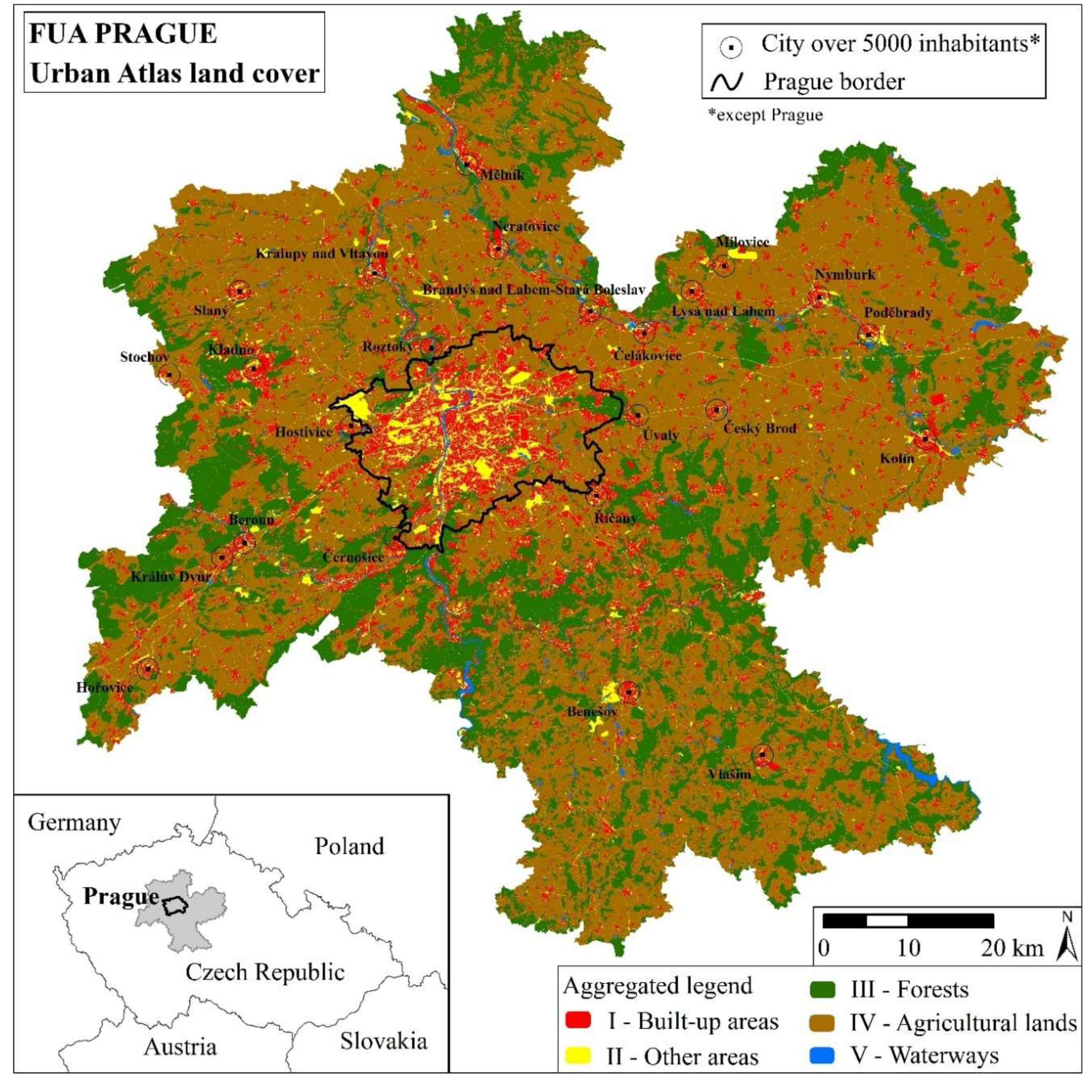
2. The Study Area
For this study, the area of the Prague agglomeration was chosen as the most suitable in Czechia for several reasons. It is the largest Czech FUA [
29], so it was assumed that it would provide a sufficient sample size to ensure the achievement of the goals of this work. Furthermore, its area provided more typologically different territories from the centre of the capital city through the periphery with a lower density of development to predominantly natural areas, which, in recent decades, have been subject to intensive changes in the use of the landscape [
23,
24]. The Prague metropolitan region provides relatively high-quality natural conditions with a large share of agricultural land, but it is undergoing very strong urbanisation and suburbanisation processes associated with population growth and intense changes in the demands of the landscape use [
23]. These processes are concentrated in specific areas and bring about varied trends in the changes in the LU/LC [
24]. The studied area was defined as the Prague FUA, excluding several cadastral units, the omission of which is explained in the methodology below. The area covered the entire region of Prague and part of the Central Bohemia region. In particular, the districts of Prague-východ, Prague-západ, Benešov, Kolín, Nymburk, Mělník, Kladno, and Beroun were included in the limits applicable to 2006 [
30].
Figure 1 shows the observed study area. The extent of this area was 6975 km
2, and it was divided into 1353 cadastral units (CU).
4. Results
4.1. Changes in the LU/LC in the Prague FUA
The areas of the UA nomenclature classes in 2006 and 2012 in the area under consideration are shown in
Table 6 and
Table A1 (
Appendix B). In 2006, the agricultural area (2) had the largest share with 60%, followed by forests (3) with 24%, and then artificial areas (1) with 15% and water areas (5) with 1%. Between 2006 and 2012, there was an increase in the artificial areas (1) of 0.6% and a decline of 0.6% in the agricultural areas (2); a smaller decrease was recorded in the forests (3), and the water areas (5) slightly increased their share.
A more detailed examination of the artificial area class shows that the increase was reflected in all of its subordinate classes, except for the construction sites (1.3.3) and the urban green areas (1.4.1), whose areas diminished. The largest increase was recorded by the very sparse area (1.1.2.4), whose area increased by about twenty times. Other sparsely populated areas (1.1.2.3), motorways (1.2.2.1), mining areas and landfills (1.3.1) and recreational and sports facilities (1.4.2) were the other major growth regions in the original area.
The areas of the KN nomenclature classes in 2006 and 2012 are shown in
Table 7. The arable land (2) accounted for 53% of the total area in 2006, followed by forests (10) at 22%, and other areas (14) at 10%. The garden (5), orchard (6), permanent grassland (7), waterway (11), and built-up area (13) classes followed with a range of one to five percent of the total area.
Between 2006 and 2012, all agricultural utilisation classes (2, 3, 4, 6), with the exception of the grassland class (7), recorded a decline, which, on the contrary, increased its area. The remaining classes under the KN database recorded increases in their areas in the given period. The other areas (14) and built-up areas (13) were the most affected at 0.3% and 0.1% of the whole area, respectively. Compared to their 2006 scale, both of these classes increased by about 3%. This characteristic was also reflected in the growth of gardens (2%) and waterways (1%). Forests expanded by about 0.2%.
4.2. Comparison of the KN and UA data
KN and UA data were compared in five LU/LC classes aggregated from the original classes of both legends (see methodology).
Table 8 shows the land use changes between 2006 and 2012 for the entire area under investigation, as recorded by both databases.
Table 9 documents the total area of each of the different classes and also indicates which classes had positive or negative differences. A positive difference represents a larger extent of the given class in the UA data and a negative difference represents a larger extent in the KN data.
Built-up areas and gardens (I) accounted for about 6% of the total area in the KN and 9%–10% of the total area in the UA; the other areas (II) represented 10% of the area in the KN, but it was around 5% of the area in the UA. When we added up the area of these two classes together, we found that there was two percent more area in the KN than in the UA. Similarly, in the water areas (V), the KN accounts for significantly more area, approximately two percent of the area surveyed, while the UA accounted for one percent. The opposite was true in the forest (III). The percentage area of forests in the total area in the UA was larger by more than 2%.
Concerning changes that occurred between 2006 and 2012 in the two databases examined, the areas of buildings and gardens, other plots, and water grew at the expense of agricultural sites. The absolute decline in agricultural land was about 4400 ha in the UA, but it was 3400 ha in the KN, a quarter less. The built-up and other areas increased in the UA as well as in the KN. Only one class recorded a contradictory change between databases: forest area decreased by 200 ha in the UA but increased by 350 hectares in the KN.
The class of built-up areas and gardens (I) was significantly larger in the UA (65,000–69,000 ha) than in the KN (41,000–42,000 ha). The area of the other aggregate class (II) in KN was more than double than in the UA data. This may be due to the fact that the UA class of agricultural areas (2) also contains non-agricultural uses, which should fall just below the other class in the KN, thus causing a larger agricultural class (IV) area in the UA compared to in the KN. The forest class (III) had about 10% more area in the UA than in the KN. This can be explained by the different methods of collecting the data: KN (de jure) and UA (de facto). The waterways (V) area almost doubled in the KN when compared to the UA data, occupying one percentage point of the total area while that of KN was two percent. There was a difference between the KN and the UA parameters, namely, the minimum mapping unit. The UA data did not include water areas less than 1 hectare or waterways less than 10 m wide. The change between 2006 and 2012 was similar in this class for the two datasets. Both sets showed a slight increase in water areas.
As shown in
Table 9, in 2006 and 2012, about 52,000 and 54,000 ha of differently classified areas (different areas) were found between the KN and UA databases, respectively. The results confirm the aforementioned assertions, where the positive difference strongly prevailed for the classes I and III, with a lower intensity for class IV. There was a negative difference in classes II and V.
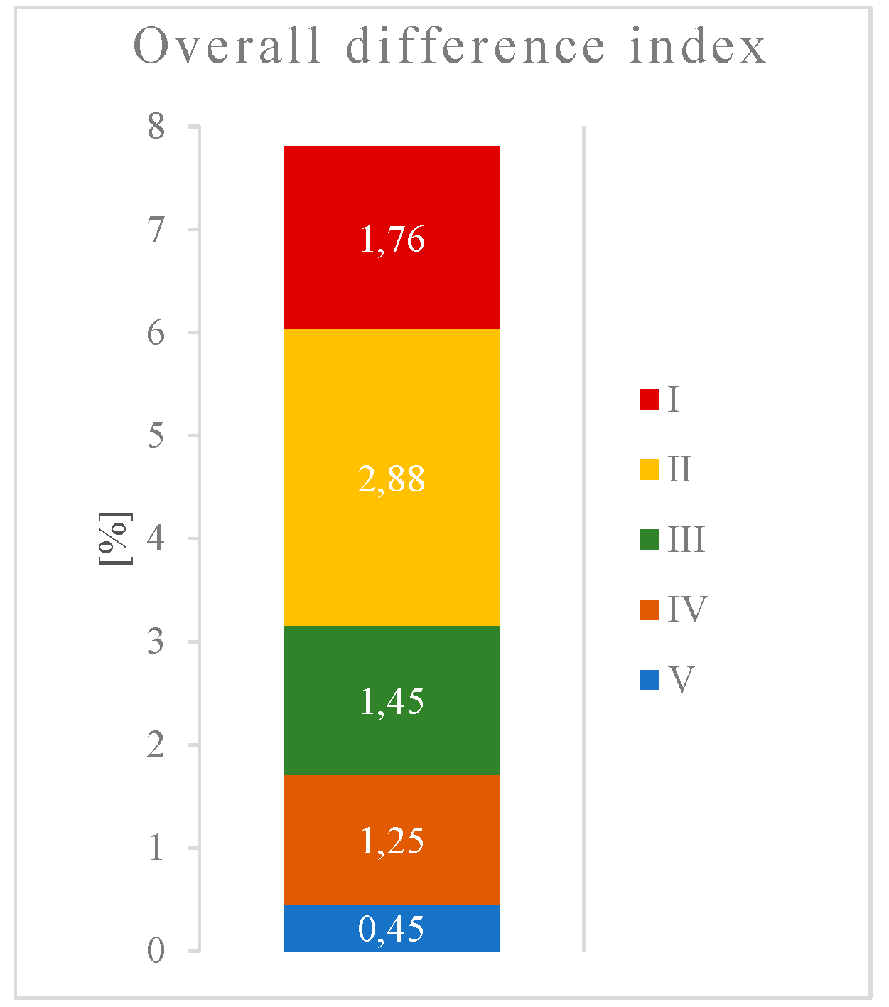
Within each unit (1329 units surveyed) and each class, the differently classified areas were calculated, and based on these differences, calculation of the DI was performed. The average value of the DI between the KN and UA data was 7.8% in 2006 and 8.1% in 2012. This means that, on average, 8% of each cadastral unit was classified into different classes in the KN and UA data.
Figure 3 shows how the individual classes contributed to the total DI in 2006. The largest share (2.88%) came from the other areas (II), the smallest (0.45%) came from water surfaces (V), and the remainder was between one and two percent.
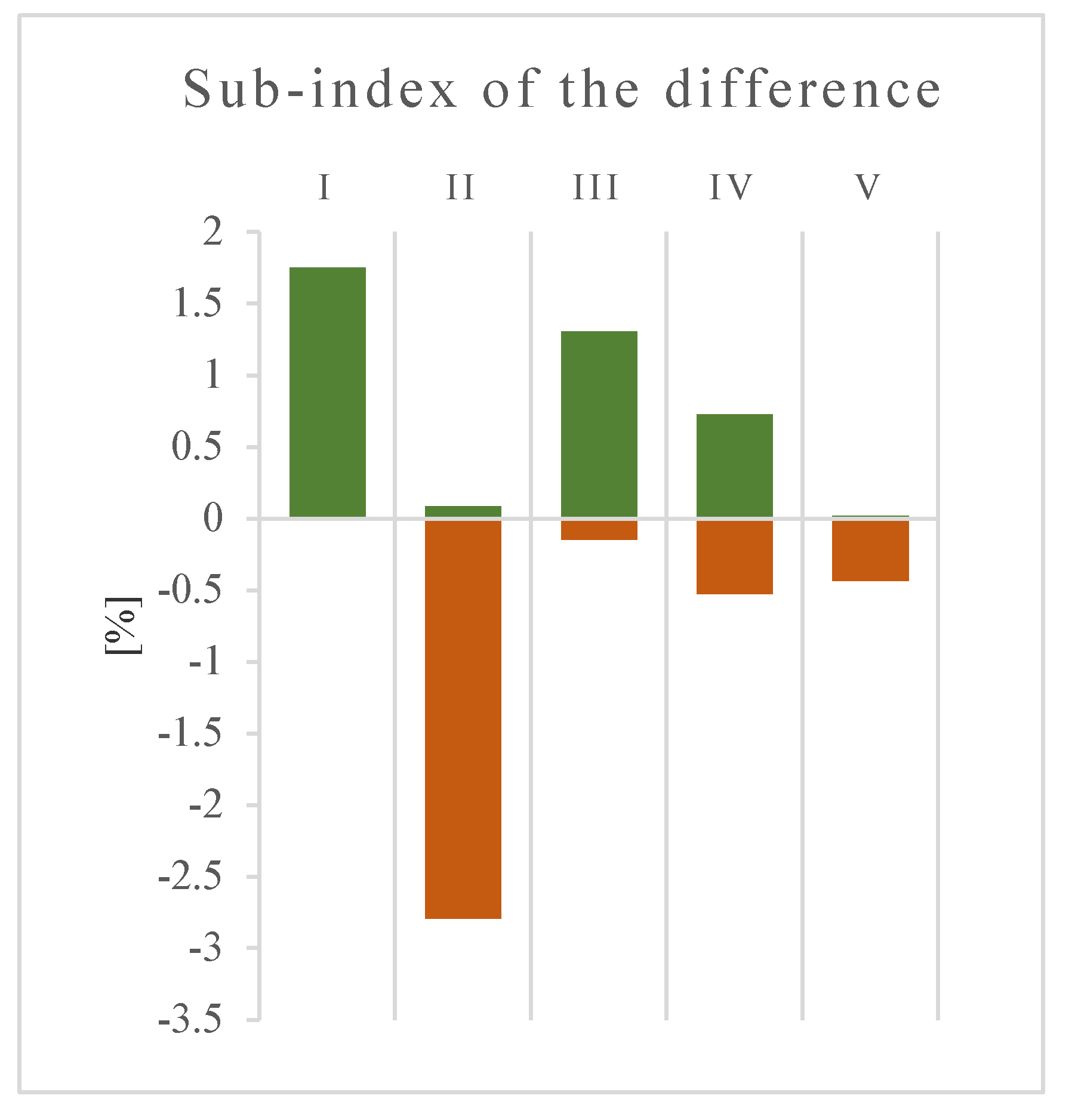
Figure 4 specifies the structure of the results presented in
Figure 3. Positive and negative differences are distinguished here.
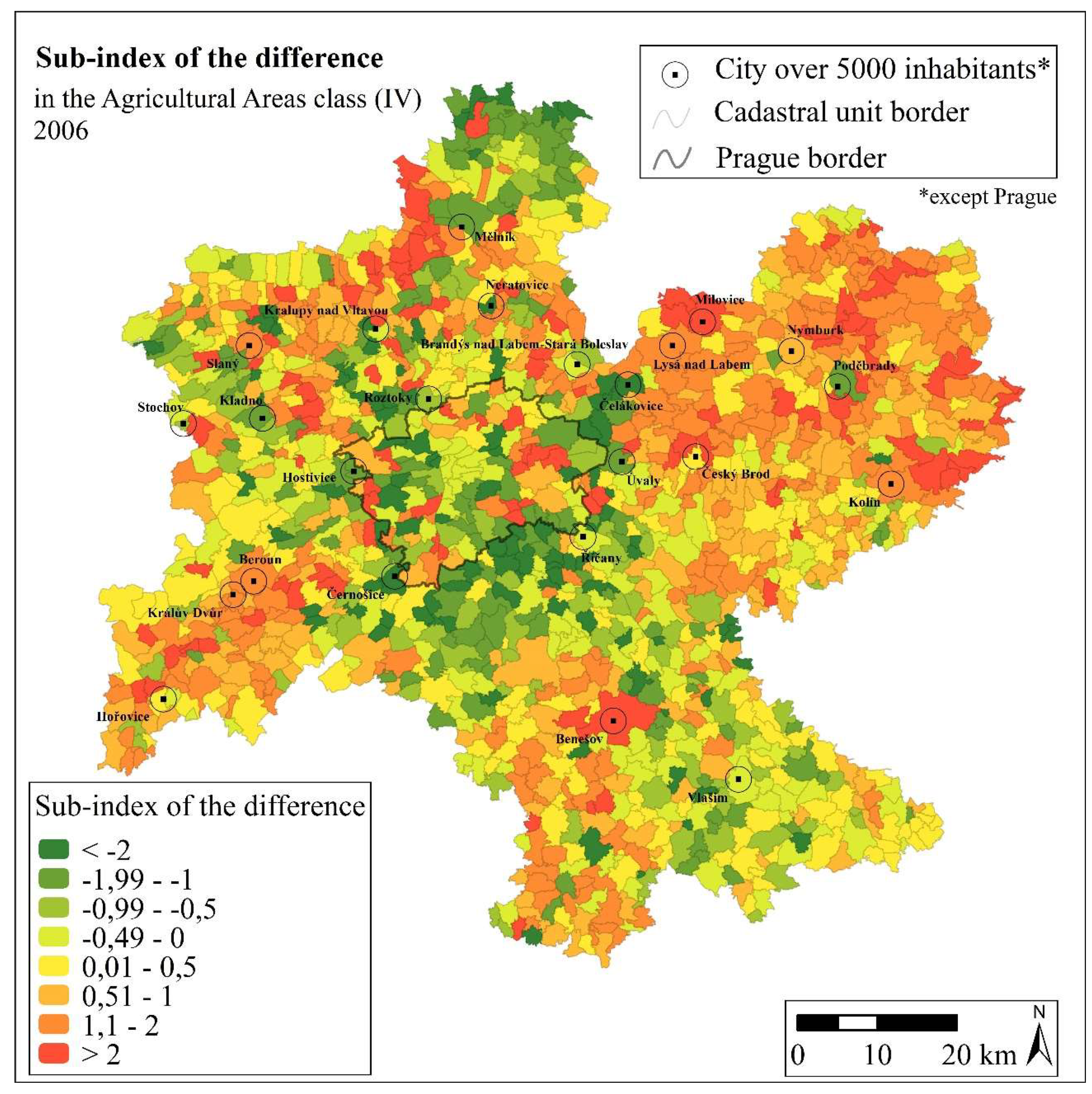
Figure 4 shows positive and negative differences in a 2:3 ratio in the Agricultural Area Class (IV) in favour of the UA. The remaining classes (I, II, III, and V) did not show any marked contradictory tendencies in the area under investigation.
The agricultural areas (IV) where the UA data revealed new development between 2006 and 2012 were larger in the KN data than in the UA data.
Figure 5 shows the spatial layout of such areas. As the results show, this was a very common phenomenon. In addition to the UA data, the total area recorded by the KN in the Agricultural Areas Class (IV) was 5916 ha in 2006 and 6783 ha in 2012. On the other hand, the extra area recorded in this class by the UA was 10,366 ha in 2006 and 10,196 ha in 2012 (
Table 9).
Concerning similarities, the greatest agreement between databases was found in category V (waterways), as can be seen from the graph in
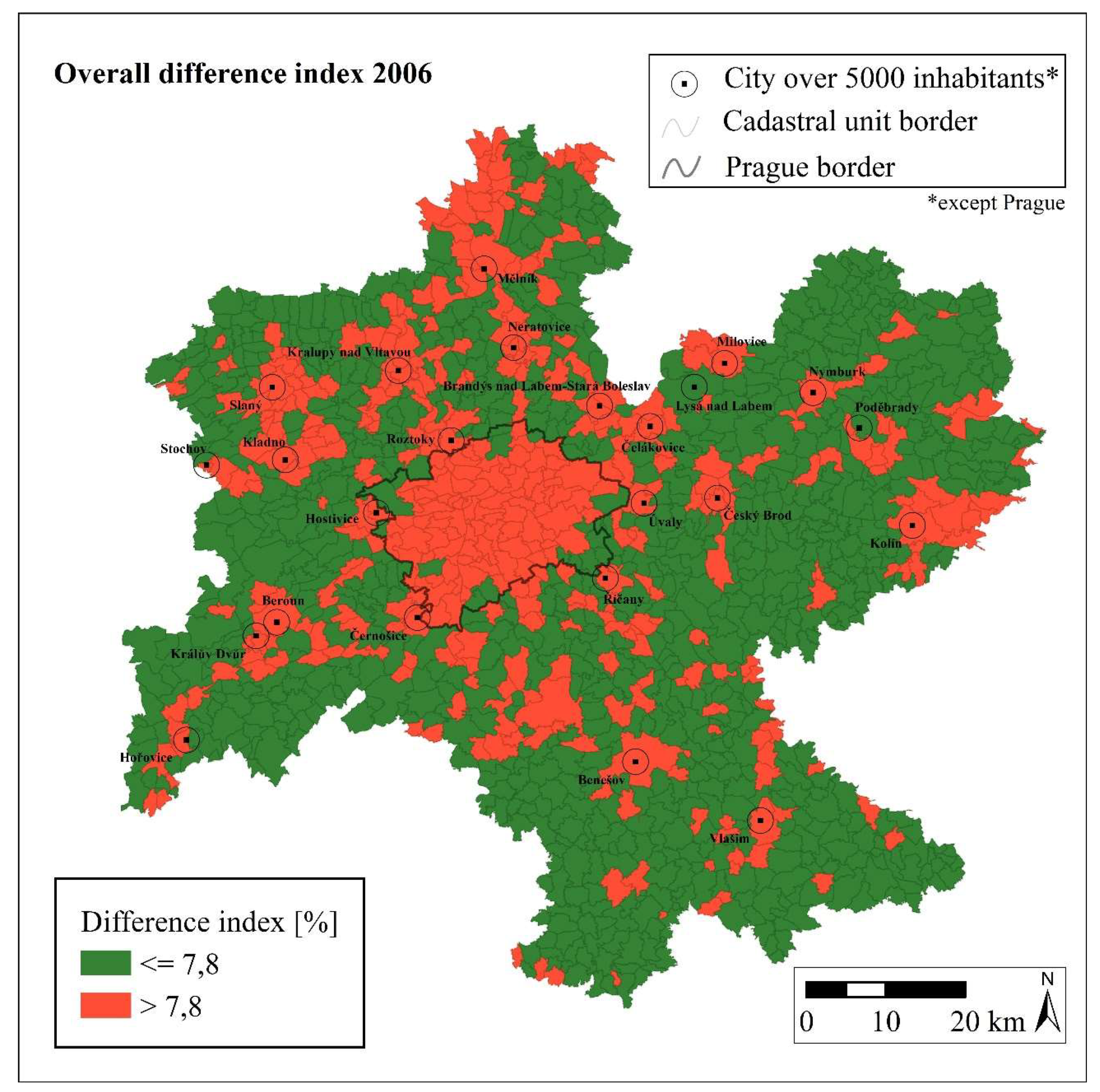
Figure 3. The small differences in this class may have been caused by the high semantic proximity in this class between the databases and the generally small area of waterways in the area of interest. A high level of similarity between databases was also found in classes III (Forests) and IV (Agricultural areas). When examining the data from individual cadastral units, it was observed that the CUs showing the highest level of correspondence were those dominated by agricultural and forest areas. This aspect is confirmed in the map in
Figure 6, which shows territorial differences/similarities. CUs were divided by the average difference index from 2006 data (7.8%) into those with above and below average DI values. The greatest agreement between databases was found for country landscape in the areas with low levels of urbanisation and suburbanisation (outside of the larger towns), which have greater percentages of agricultural and forest areas.
4.3. Comparison of the Databases in the Selected Cadastres
The analysis of the selected CUs in this part documents the differences on a detailed scale level (on a parcel level). These analyses make it possible to better understand the differences, and, in combination with additional data, contribute to the explanation of the causes. To give a detailed understanding of the differences and possibilities of interpretation and explanation, we selected cadastres where the situation/location of the classes in both databases could be compared with aerial images.
4.3.1. CU Háje
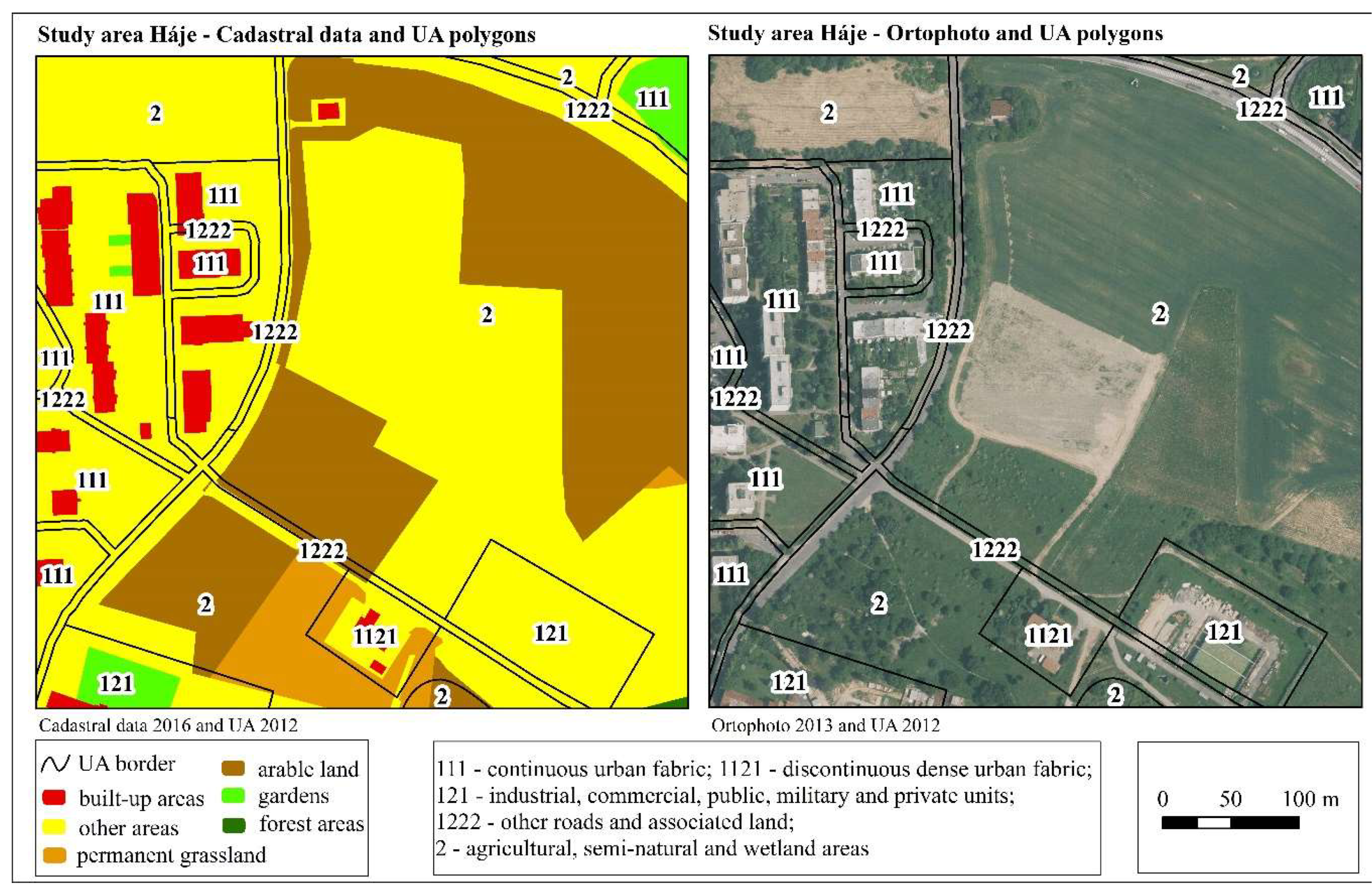
The CU Háje was chosen as an exemplary unit with differences in the class of agricultural areas (IV): a larger area of agricultural land (IV) was found in the UA at the expense of class II (other area) in the KN. The CU Háje is located in the south-eastern outskirts of Prague. The DI values (rounded to percentages) in 2006 and 2012 are shown in
Table 10.
The maps and orthophotos show the locations of problematic parcels (
Figure 7). Most of the areas classified as agricultural areas (2) in the UA and as other classes (14) in the KN are really natural in nature and, especially in the eastern part of the section (
Figure 7), they form a unitary unit with parcels in the KN that are listed as agricultural (2). In these areas, it is interesting that many of them are divided into smaller plots in the KN, remarkably resembling the structure of the urban areas. Most of the areas mentioned are registered as other classes in the KN. Obviously, for a large number of areas, agricultural activity continues to be carried out; therefore, their classification into the other class may be considered to conflict with the definitions of the cadastral legend. The remainder of the difference in the data is due to the fact that urban areas (1.1) in UA include buildings as well as gardens and other areas, which are defined separately in the KN. The area in the UA described as continuous urban area (1.1.1) is mainly classed as other areas and built-up areas in the KN. When looking at the orthophoto map, it is clear that the definition of built-up areas is narrow within the KN, that is, only the areas on which the building is built are included, while the rest of the definition referring to the yards or entrances is not taken into account.
4.3.2. CU Hodkovičky
The CU Hodkovičky is located in the southern part of Prague, relatively close to the centre. A larger agricultural area was recorded by the KN compared with the UA. DI values are shown in
Table 11.
The areas that have a difference in Class IV in the CU Hodkovicky are classed as arable land (2) in the KN, but in the UA they are classified as urban green areas (1.4.1) and sports and recreation areas (1.4.2) (see
Table 10). Approximately half of the disputed area includes golf courses, which are mostly recorded as arable land (2) in the KN. Golf courses should be included in the KN under the other class (sports area). A significant part of the different areas is also located in the vicinity of the individual recreation facilities, which are registered as built-up areas in the KN (13), but their surroundings are recorded as arable land (2). All of this area is classified as a sports and recreation area in the UA (1.4.2). The rest are areas of natural character, often with growing vegetation in the UA, which is marked as urban greenery (1.4.1) in the KN, again partly in the arable land class (2) and partly in the other areas class (14). According to the KN, sports grounds are reserved for use within the classes of other areas as well as for greenery forming units with buildings. There is, therefore, a clear conflict between recorded use and reality.
4.3.3. CU Vysočany
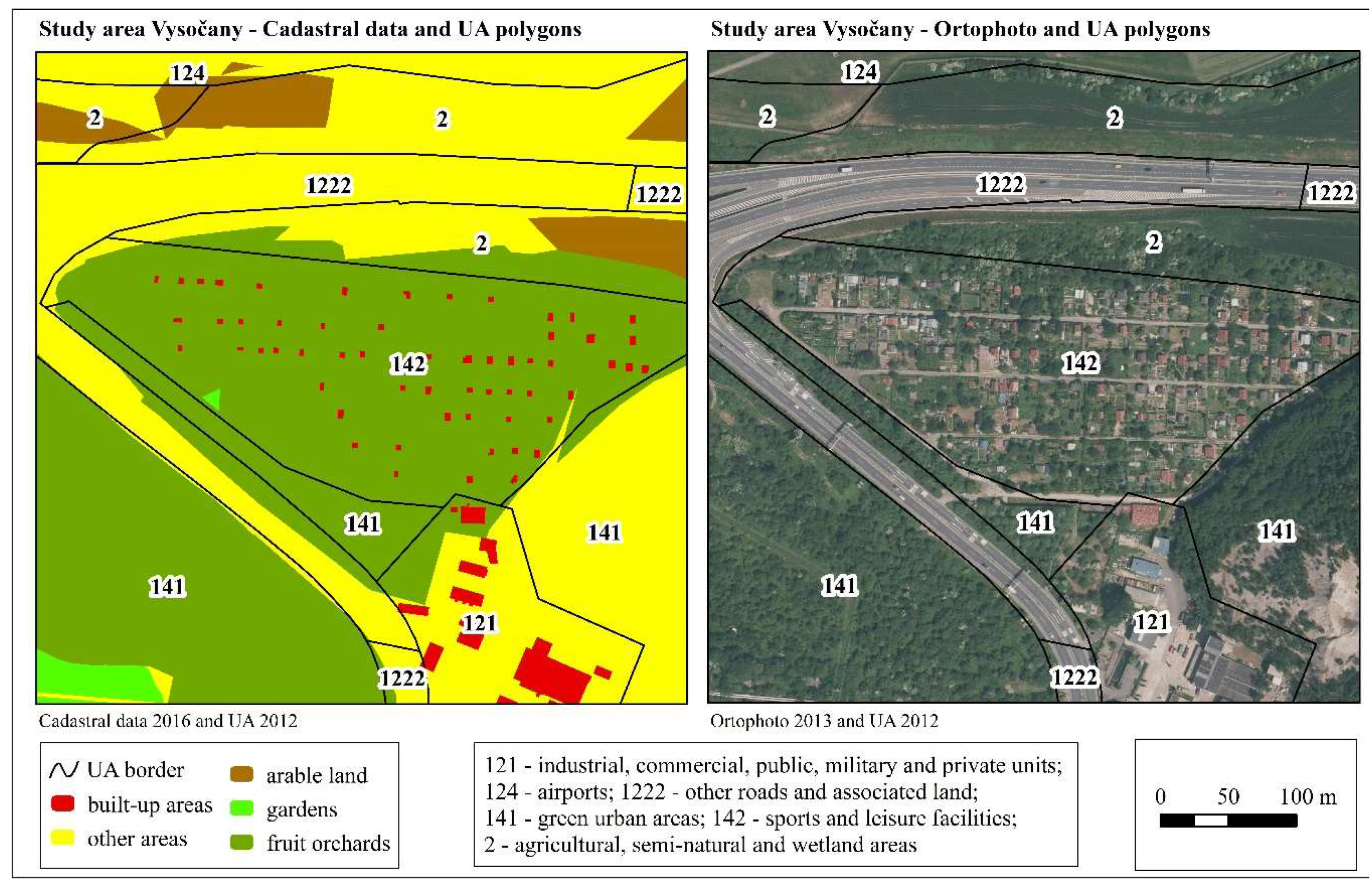
In the CU Vysočany, the differences in agricultural areas (IV) are mainly due to the areas classified under the heading of orchards (6) in the KN and under urban areas (1.4.1) or recreational (1.4.2) green areas in the UA. The CU Vysočany is situated on the northern outskirts of Prague. Most of the sites consist of parcels with a continuous growth of fruit trees. In this case, it is possible to look for a potential conflict with the definition in the UA, since fruit orchards should be classified under agricultural areas (2). In this case, however, the same rule applies as for forests: if the areas are surrounded by polygons of artificial area classes (1), they can be included in the urban green class (1.4.1). The individual recreation facilities are mapped as recreational greenery (1.4.2) in the UA and as fruit orchards (6) supplemented by built-up areas (14) in the KN (see
Figure 8). Such a classification within the KN is in conflict with the definition because, although part of the area consists of trees, they are not used for agricultural purposes, but rather, are used for recreational purposes. Another major problem is the absence of the road network and some buildings on the cadastral map.
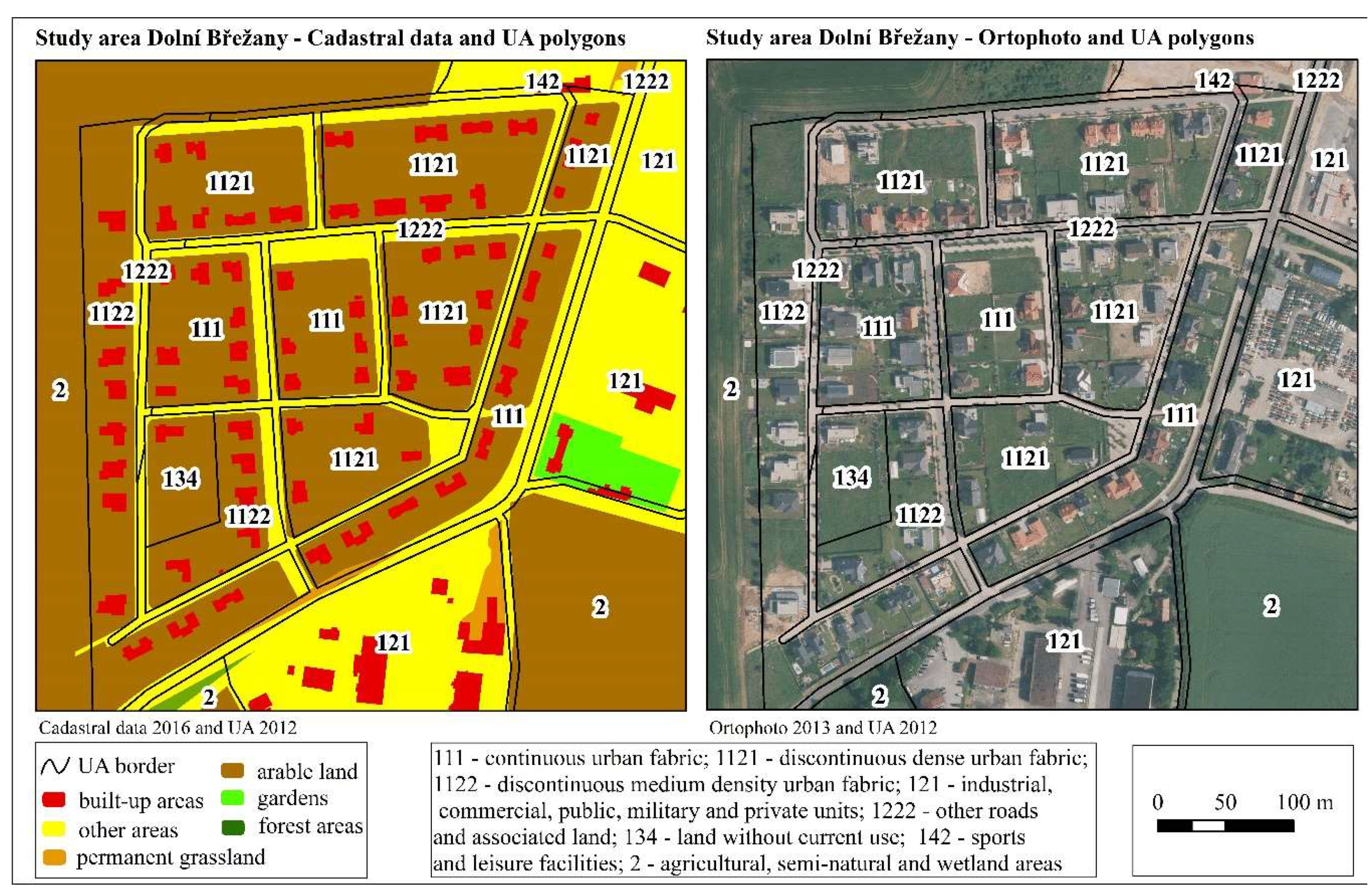
4.3.4. CU Dolní Břežany
The CU Dolní Břežany is a representative of the situation where the differences in the agricultural area (IV) class often occur in the areas around the buildings, which are listed as urban areas (1.1) in the UA but are in the arable land class (2) in the KN. Such a situation is a relatively frequent phenomenon in suburban areas where dynamic development of residential areas took place after 1990. This CU adjoins the southern border of Prague. The DI of this CU is shown in
Table 12.
As can be seen from
Figure 9, the road network and individual buildings are recorded in the KN (with few exceptions), but the surrounding area of the buildings used as a garden is referred to as arable land (2), which is clearly inconsistent with the definition of this class. These areas are not used for agricultural production, meaning that they should be included in other classes (14).
5. Discussion
Different disciplinary and scale approaches have led to the creation of many databases with different focuses, each with its own classification nomenclature. With the dynamic development of geoinformation technologies and monitoring systems, a large number of different LU/LC databases have been created on different scales. The end-users of these databases should know their characteristics and limits to avoid potential mistakes resulting from inappropriate combinations and interpretations. Using this point of view, the evaluation of the different characteristics of nomenclatures of the KN and UA was the main focus of this study. During the evaluation of the data, thematic aggregation and spatial aggregation were undertaken. The advantage of the chosen procedure is that it minimises the problems caused by spatial inaccuracies in the data under review (see, for example, Štysová 2015) [
49]. For a summary of the quantification of differences, a statistical indicator, the DI, was selected to determine the differences in conversion to the total area. The DI has been widely using in studies of long-term land use changes, e.g., Bičík et al. (2010) [
48]. This study implemented and tested this index in the evaluation/harmonisation of LU/LC nomenclatures.
In the case of the largest differences observed across the whole area, it was confirmed that the country landscape (areas outside of the bigger towns where population stagnation and low levels of economic and residential development have occurred) has a below-average rate of differences in both databases. These areas are located outside the main urbanisation/suburbanisation axes. It was also established that cadastral units with higher levels of similarity are dominated by agricultural and forest areas. This shows that smaller differences typically occur for agricultural lands, forests, and waterways. Concerning the types of areas evaluated as problematic, vegetation without agricultural or forestry use can be a source of conflict between the different LU/LC data sources. Significant disparities have been observed in “other areas” of the KN. Problematic areas include sports grounds, photovoltaic power stations, and areas surrounding family houses. Similar findings were shown by Bach et al. (2006) [
10] and Neumann et al., 2007 [
11], who also identified significant confusion in the transition areas between forests and other classes of less-developed vegetation.
In suburban areas where the most intense changes to the LU/LC were localised, significant differences between the two databases were identified, in accordance with the hypothesis. Our results are consistent with the cited literature [
3,
12]. The out-of-date nature of the KN is the most probable cause of the differences in both non-compliance and ignorance of the obligations imposed on owners in this context by the cadastral law [
19]. This is due to the fact that data in the KN were collected from announcements of land ownership changes. The reasons for the inconsistency in the number of buildings in the residential areas between the KN and UA data can be attributed to this fact.
The evaluation of the data on different scales (an analysis of the whole area of the Prague metropolitan region and a detailed analysis of the selected cadastral units) allowed us to conduct a deep investigation of the content of databases. Using this approach, we managed to prove the existence of significant errors in the evaluated databases. As far as the KN is concerned, these errors mainly involve systematic overstatement of the size of the agricultural use class to the detriment of either the surroundings of built-up areas with residential use (gardens, handling areas, entrances, etc.) or extensive sports grounds, especially in areas with high growth dynamics. To a lesser extent, they involve the devaluation of forests, which are included in other areas. For UA data, errors mainly involve the inclusion of sites across different dense urban areas, for which an inconsistent approach was used between the years 2006 and 2012. This is followed by a larger proportion of artificial areas in the respective LU/LC classes than are present in the real state. The increase in Class 1.1.2.4 areas in the UA 2012 was due to a new development. Thus, the classification does not contradict the nomenclature, but, nevertheless, some inconsistency in the methodology is shown.
If we focus on the strengths and weaknesses of both databases, it is possible to identify with the conclusions of Bach et al. (2006) [
10], who stated the cause of some of the mismatches between the cadastral data and LU/LC maps is a generalisation of the UA database. This phenomenon has been confirmed, particularly in water areas. McConnell (2002) [
50] and Büttner (2016) [
51] reported the problem of mixing LUs and LCs in nomenclature as one of the main complaints directed by LU/LC database users. As far as the KN is concerned, this ambivalence is quite visible, e.g., in the other classes. This class combines affected anthropogenic surfaces and areas with shrubs. In the case of the KN, the primary task is to record the legal status of the land for the purposes of state administration, i.e., what the plot is used for, regardless of its physical surface. It has been proven that the cadastral evidence is outdated and it has a limited ability to show LU/LUC changes in areas with high growth dynamics due to new developments. The official cadastral records document lower shares of built-up areas compared to the UA data, and the largest disagreements are located in the most dynamically developing suburban areas (where a larger number of newly built areas are expected). In the context of the current level of technology and knowledge in the field of geoinformatics and RS, it is necessary to address the idea of whether it would be appropriate to use more intensive RS in the process of KN data revision. To achieve this, it is necessary to improve the temporal resolution of the databases based on the RS (Urban Atlas), which would need to be updated annually.
Foody (1999) [
52] and Jansen (2005) [
28] stated that one of the fundamental principles in relation to the nomenclature is that their classes are both exclusive and they continually cover the entire real situation on the ground. The KN data addresses the issue of the continuity of its nomenclature by introducing the other areas class, which can include any area that does not match any of the previous classes. The UA methodology states that the classification takes place in phases using a tree structure, which also ensures continuity. In this respect, there was a problem with forest stands, for which both the UA and the KN have the same class and, to a certain extent, the same definition, but both nomenclatures allow, under certain circumstances, the inclusion of such surfaces in other classes (UA into the urban greenery class, KN between other areas). The built-up areas and garden areas were significantly larger in the UA (65,000–69,000 ha) than in the KN (41,000–42,000 ha). The reason for this is that the polygons of the residential area in the UA consist of buildings and their surroundings. These surroundings are generally registered as gardens in the KN, but they may also be included under the other areas class (class 14) in the KN, such as greenery or parts of the road.
A factor that could have had some influence on the results of this study is the choice of time horizon. Cumulative cadastral data values are valid on the 31st of December of the year of study, while the UA data have a time tolerance of +/– 1 year [
41]. It is also necessary to take into account the fact that the thematic accuracy of the UA database is limited. Although an accuracy level of 80% was met for both time horizons (specific values ranging between 80% and 90%), partial results could be affected by this factor. The results of the comparison of the data sets were undoubtedly influenced by the choice of territory within Czechia where the comparison was made. It is possible that the results would be different in other parts of the country. It would, therefore, be appropriate to verify them in other areas, for example, in regions with less intense changes to the LU/LC than those of the surrounding area of Prague. We also recommend that further studies are carried out to compare the KN data with UAs in other countries.
Although the chosen methods have yielded many relevant results, further study of classic spatial overlapping of the KN and UA data is recommended. More attention should be paid to the geometric differences in both databases. It would also be worthwhile to carry out a deeper assessment of the causes of the problems encountered, in particular, those of the KN. Due to the fact that data in the KN arise on the basis of the announcement of land ownership changes, it would be useful to look for more detailed causes of inconsistency in the cadastral data compared with the actual state in relation to the land owner’s role. The possible cause of the out-of-date nature of the KN is both non-compliance and ignorance of the obligations imposed on owners in this context by the cadastral law [
19]. Motivation for deliberate non-compliance with this law may be economic profit. Payment of taxes and fees for removing land from the agricultural land fund may be a relevant cause of the owners not officially changing land use in the cadastre, as the annual tax is higher for other areas than for arable land, as was noted by Sláma et al. (2018) [
53]. The legislative and legal issues in relation to the LU/LC data in the KN, discussed in several places in this paper, would certainly be an interesting subject for interdisciplinary research. Last but not least, an awareness about the accuracy and limits of the LU data in the cadastre of real estate is important from the point of view of reporting land use, land use change, and forestry data (LULUCF) for climate action, e.g., legislation and strategies for reducing greenhouse gas emissions. The data from the cadastre of real estate is still the main source for determining LU/LC changes as part of climate-change-related actions and strategies [
54].
6. Conclusions
This study evaluated the thematic content of the UA database and data from the Czech cadastre of real estate in the Prague metropolitan region between the years 2006 and 2012 with a focus on the meaning of the nomenclature used by both datasets. The data were processed using approaches with different levels of thematic harmonisation and statistical tools that quantified the similarities within the researched data. The study tried to introduce novel methods into the evaluation of differences/similarities in LU data in different databases. The methods of evaluation used for LU data were based on an aggregation approach and modified DI values (the overall difference index and the sub-index of the difference). During the processing and comparison of the data, thematic aggregation and spatial aggregation were undertaken, meaning the area of the complexes in the individual classes of the given nomenclature was summarised for each cadastral unit. Areas with a high degree of dissimilarity and similarity were found, further examined, and interpreted in detail. The evaluation of the LU data at the different scale levels (an analysis of the whole area of the Prague metropolitan region and a detailed analysis of the selected cadastral units) allowed us to carry out a deep investigation and interpretation of the content of databases. It was proven that the differences between both datasets are significant and that the databases share certain characteristics. Most of the differences were found to be distributed in the classes of built-up areas, gardens, and other areas. Smaller differences were found for waterways, agricultural lands, and forest. In suburban areas, where the most intense changes to the LU/LC were localised, significant differences between the two databases were identified. It was found that the cadastral evidence is outdated, and it has a limited ability to record LU/LUC changes in areas with high growth dynamics due to new development. The results enhance the scientific knowledge about the uniqueness, comparability, and complementarity of the UA and KN databases, which can facilitate decision-making about the options of their use with the intention of raising awareness of their limits, strengths, and weaknesses. In the context of the current level of technology and knowledge in the field of geoinformatics and RS, it is appropriate to use more intensive modern monitoring tools in the process of the revision and evaluation of LU data in the KN.


