Abstract
Two soil mapping methodologies at different scales applied in the same area were compared in order to investigate the potential of their combined use to achieve an integrated and more accurate soil description for sustainable land use management. The two methodologies represent the main types of soil mapping systems used and still applied in soil surveys in Greece. Diomedes Botanical Garden (DBG) (Athens, Greece) was used as a study area because past cartographic data of soil survey were available. The older soil survey data were obtained via the conventional methodology extensively used over time since the beginnings of soil mapping in Greece (1977). The second mapping methodology constitutes the current soil mapping system in Greece recently used for compilation of the national soil map. The obtained cartographic and soil data resulting from the application of the two methodologies were analyzed and compared using appropriate geospatial techniques. Even though the two mapping methodologies have been performed at different mapping scales, using partially different mapping symbols and different soil classification systems, the description of the soils based on the cartographic symbols of the two methodologies presented an agreement of 63.7% while the soil classification by the two taxonomic systems namely Soil Taxonomy and World Reference Base for Soil Resources had an average coincidence of 69.5%.
1. Introduction
Soil surveys provide a source of information and an inventory of soil parameters of an area of interest assisting land users to make accurate predictions for the response of a specific land to a certain use [1]. An integrated soil survey delineates the groups of soils of a region and describes their characteristics by using a specific mapping and classification system. Taking into consideration this information, the behavior of soils and their interaction with various land uses can be foreseen [2]. Therefore, there is an interdependent and interactive relationship between soil surveys and soil mapping [3] since the information of soil properties and their spatial distribution, given by detailed and accurate maps, are necessary for evaluation and land suitability analysis [4]. The landscape-soil relationship is reflected and emphatically imprinted in soil surveys and soil maps [5] and therefore together they consist an important driver for sustainable land management [6].
There are generally two approaches to mapping the soils, the modern and recently increasingly used digital soil mapping (DSM) [7,8] and the traditional soil mapping. Traditional soil mapping is conducted on the basis of Soil Mapping Unit (SMU), which is concerned as a distinguishable spatial object that delineates areas on the earth surface with similar physical and chemical properties [9]. This approach indicates a certain degree of subjectivity in the delineations of SMUs [10] since their nature is also transitional [11]. Actually, the physical soil in the landscape is segregated into discrete entities via the SMUs [12], consisting of one or several Soil Typological Units (STUs) [13], that represent soil volumes having the same arrangement of soil horizons (soil pedon) [14]. As the scale becomes more detailed the number of STUs in an SMU diminishes up to the level of very detailed mapping, where the SMU boundaries are identical to STU boundaries [14]. At the beginnings of soil mapping in Greece, due to a lack of technology, the initial delineation of SMUs was carried out on topographic backgrounds during field crossings of the mapped area and related observations of the environment [15]. With the progress of technology, new computer-based techniques of preliminary delineation of SMUs were developed [16]. SMU’s delineations are based on the principle that the same factors of soil genesis create repeated geomorphological structures that can be identified both on a combination of various cartographic backgrounds and on the Earth’s surface [2]. Those repetitive patterns are reflected in soils under the effect of soil-forming factors and can be identified at scales from continental to microscopic consisting the cornerstone for soil identification and mapping at various scales [2]. So, a SMU corresponds to a specific area in the map as well as to a specific part of the landscape in the physical environment [17].
The size of SMUs is determined from the mapping scale and the specific purposes of soil survey. Specifically, the minimum legible delineation (MLD) is defined as the smallest distinguishable area of any map that can be legibly delineated. MLD conventionally represents an area of 0.4 cm2 independently of the mapping scale [1]. According to the mapping scale, the minimum legible area (MLA) that can be defined on a map, is totally connected and emerges from MLD. In terms of investigating which mapping scale is the most appropriate for the composition of a map for a specific soil/land use, the MLA must be equal or smaller than the minimum area of mapping interest for this specific soil/land use [1]. Taking into consideration the above-mentioned concepts, soil mapping of the same area in semi-detailed and detailed scales will result in the creation of few and extended SMUs in the first case and to more and less extended SMUs in the latter case, respectively. According to Food and Agriculture Organization of the United Nations (FAO) guidelines technical paper [18] semi-detailed soil surveys are typically at scales from 1:25,000 to 1:50,000, while detailed soil map’s scales ranging from 1:10,000 to 1:25,000. The mapping scale largely influences the accuracy of soils grouping in SMUs. Detailed and semi-detailed soil maps are widely used for agricultural applications such as land resources assessment and land use planning [19].
The soil map of a country constitutes a basic national and infrastructural project for agricultural development and for the sustainable management of the primary sector. [20]. In Greece, the first actual integrated efforts for soil mapping have been carried out since 1977 through the implementation of a relevant law (Government Gazette Issue 186/A’/30-6-1977) with economic assistance from United Nations and Europe. Nowadays and due to the previous efforts, a plethora of soil surveys exist, mainly in detailed scale (1:5000–1:20,000) [21], which cover approximately the 15% of the agricultural areas in a fragmented pattern. Quite recently [22] the Greek Ministry of Rural Development and Food (Greek Payment and Control Agency for Guidance and Guarantee Community Aid, 2014) has funded the compilation of the national soil map in a semi-detailed scale (1:30,000) which includes approximately the 85% of the agricultural areas of the country. The results of the old (before 2014) and the new (2014) soil mapping of the agricultural areas in Greece present some spatial overlaps but mainly the two efforts complement each other as far as their spatial distribution is concerned. Summarizing, today, despite the numerous soil surveys in agricultural areas for which have been utilized considerable financial resources and a lot of working time there is not available a united, normalized and integrated soil map of the agricultural areas of Greece.
The objective of this study was the comparison of the two soil mapping systems (old and new) in order to investigate the potential of their combined use utilizing the already existing soil maps in Greece to complete the national soil map of the country. Particularly, the comparison focused on—(a) the volume of soil information that the two systems can record; (b) the reliability of the conclusions drawn from them on soil’s characteristics and land utilization and (c) the potential for combining them to create final and integrated thematic maps; combining the detailed spatial information of conventional soil mapping (old) and the smaller-scale spatial information of current soil mapping (new) in the study area of the DBG.
2. Materials and Methods
2.1. The Study Area
The Diomedes Botanical Garden (DBG) is located in Attica (Greece) west of Athens, covering an area of approximately 175 ha (Figure 1). It is mostly a sloping area with slopes ranging from 2%–65% and is crossed by few small gorges and waterways. The DBG is a social welfare area including a private legal entity under the administration of National and Kapodistrian University of Athens. This garden is covered by natural vegetation, which consists mainly of Pinus halepensis, Pinus brutia, Cupressus sempervirens, Quercus coccifera, Pistacia lentiscus whereas a significant part of the garden is occupied by “phrygana” with the most representative species to be Sarcopoterium spinosum, Cistus spp., Phlomis fruticosa, Euphorbia acanthothamnos, Coridothymus capitatus and Satureja thymbra. The chasmophytic vegetation of the garden is also remarkable consisting of Campanula celsii subsp. celsii, Inula verbascifolia subsp. methanaea and so forth [23]. The garden was established at 1951, in the west region of Athens, north of Aigaleo mountain in a hilly area where the dominant parent material is limestone, followed by schist [24]. The study area is characterized by a Mediterranean climate, with long hot and dry summers and moderately wet and cold winters. The annual precipitation is ranging between 259 and 576 mm, whereas the average annual temperature is approximately 19.8 °C [25]. This study area was selected due to the availability of old mapping data and to its proximity to the Agricultural University of Athens (AUA) facilities where most of the co-authors work. The lack of financial assistance in completing this study had also a decisive influence in the selection of the study area.
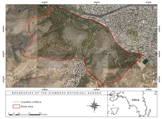
Figure 1.
The boundaries of the study area located west of Athens.
2.2. Conventional (Old) and Currently Applied (New) Soil Mapping Methodologies in Greece.
According to the conventional soil mapping system, SMUs were delineated in the field by using topographical and geological maps of the interested area and the field work was partially confirmed afterwards by laboratory soil analyses. Under the principles of the conventional soil mapping system, topographic maps in a detailed scale (1:5000–1:10,000) [26] were the basic backgrounds for the initial delineation of SMUs in the field. Actually, in this mapping methodology the preliminary delineations of SMUs boundaries were carried out based on the detailed cartographic background of the topographic map and then were identified on the basis of geological maps, macroscopical field characteristics and measured soil properties. This kind of delineation method is called physiographic [27] since it identifies the repeated geomorphological patterns depicted from the combination of the topographical, geological and vegetative characteristics which consist a physiographic region. The final obtained soil data originated from field observations including both description of representative soil profiles accompanied by soil sampling for laboratory analysis and drilling holes by augers at distances depending on the scale of soil mapping [28,29,30]. The soil survey system was developed after extensive studies and significant experience in the countryside, taking into consideration the needs of cultivation practices and the evaluation for various land uses [31]. In this context, soils characterized according to their taxonomical category under the principles of United States Department of Agriculture (USDA) Keys to Soil Taxonomy [32]. The specific key consists of 6 taxonomic categories with increasing detail from the level of Order to the level of Series (Order, Suborder, Great group, Subgroup, Family, Series). The majority of the soil surveys compiled via the conventional methodology (old) in Greece were published at a scale ranging from 1:5000 to 1:20,000 [20]. According to this methodology, developed by Yassoglou et al. [21,31], the soils were initially classified to the taxonomic level of Great group [33] or, in some cases, to the level of Subgroup and afterwards were subdivided using a set of soil parameters (depth, texture and so forth) which determine soil productivity and management (Families and Series characteristics, in the broad context), in order the soil map to be published in a semi-detailed scale. Finally, SMUs were coded using a mapping symbol in which soil properties were designated by alphanumeric characters [34]. The alphanumeric expressions of the conventional method map symbol for the alluvial plains or the lowlands of Greece correspond to eight (8) different descriptive soil parameters, which are representative of the SMU properties and referred to: the degree of drainage of the soil profile, soil texture at depths 0–25 cm, 25–75 cm and 75–150 cm, slope gradient, degree of erosion, presence of carbonates in the soil profile and taxonomic characterization, through symbols of Soil Taxonomy, referring to soil Order, Suborder and Great group/Subgroup (Appendix A, Table A1).
The criteria for the different soil Orders include properties that reflect major differences in the genesis of soils such as the presence or absence of diagnostic horizons. The soil Suborders within an Order are discerned on the basis of any soil property which can influence the absence of horizon differentiation as for example the soil moisture regime. Great group category is a subdivision of a suborder in which all the principal soil properties of the soil solum are considered collectively such as the number and the kind of soil horizons [30], the moisture and the temperature regimes [35]. Subgroup category identifies distinctive soil features among various soils within a soil Great group [36].
The previous described methodology for detailed soil mapping introduced by Yassoglou et al. [21,31] used a different, more limited in extent and information, mapping symbol for the hilly or mountainous residual soils of Greece. This symbol records seven (7) descriptive soil parameters (the degree of drainage of the soil profile, parent material, soil depth, slope gradient, degree of erosion, type of vegetation and taxonomic characterization). The two cartographic symbols of the conventional method have four (4) soil properties in common and differ in five (5) properties those of soil texture and inorganic carbonates for the lowlands and parent material, soil depth and vegetation type for the hilly soils. (Appendix A and Appendix A.1., Table A6 and Table A7). The mapping process for the hilly soils symbol follows the principles outlined above.
In the framework of the new soil mapping system (currently applied), SMUs are preliminarily delineated in a satellite orthoimage background or in an ortho-rectified photomap, usually of a semi-detailed scale, using Geographic Information System (GIS) software. The delineation of SMUs in this method is conducted on the basis of the image tone analysis macroscopically or by using image analysis techniques. Topographic, geological and vegetation maps are also used auxiliary for the preliminary delineation of SMUs. As in the case of the conventional method this kind of SMU delineation is in the context of physiographic method [27]. This soil mapping system uses geometrically corrected satellite images and geological as well as vegetation maps in semi-detailed scale (1:30,000–1:50,000) as its main background for the preliminary draw of SMUs. As in the conventional method, the finalization of SMU limits is carried out by certain morphological soil properties identified macroscopically in the field accompanied by both detailed description of the soil profiles and by laboratory analyses of selected soil samples. The mapping symbol of the currently applied methodology consists of coded letters and numbers presenting the following fourteen (14) soil properties: drainage conditions, soil texture at depths of 0–25 cm, 25–75 cm and 75–150 cm, slope gradient of soil surface, soil depth, rock fragments on soil surface, parent material, degree of soil erosion, presence of inorganic carbonates, limiting layers, electrical conductivity, soil alkalization and soil taxonomic unit [22] (Appendix A, Table A1). The taxonomic classification of soils in the context of the new soil mapping method is carried out in accordance with the rules of World Reference Base for Soil Resources (WRB) Taxonomy System [37]. The WRB system consists of two taxonomical categories in increasing detail from Reference Soil Groups (RSGs) to Principal and Supplementary Qualifiers. RSGs are defined according to primary soil-forming processes and the subsequent diagnostic soil features, excepting the case where the parent material is of prominent significance. At the second level, soil units are differentiated according to any secondary pedogenetic process that has a great influence on primary soil features. Qualifiers are subdivided in Principal Qualifiers (PQs), describing typical characteristics of RSGs and Supplementary Qualifiers (SQs), which describe additional characteristics of them [37]. The WRB classification system is recommended to be used only in soil mapping at scales from 1:250,000 to 1:1,000,000 indicating the Reference Soil Group name plus the first three PQs ranked in an order of importance with the most significant PQ placed closest to the name of the RSG [37,38]. However, as in the conventional method, new soil mapping approach also uses a combination of specific soil parameters in its mapping symbol that eventually lead the delineation of SMUs to a semi-detailed scale.
2.3. Soil Mapping of the Study Area with the Two Methods
Prior to the official soil mapping of the country (1977) the first attempt for soil mapping conducted on the study area of DBG at 1976 via the conventional soil mapping method [26]. Following the prompts of the old mapping method SMUs were delineated locally in the field using a detailed (1:5000) topographic map (Geographical Military Service of Greece—GMS) as the basic cartographic background and utilizing observations from the natural landscape (geology, soils, vegetation) in combination with geological information provided at 1:50,000 scale [24]. SMUs were delineated on the basis of the attributes of the two mapping symbols (lowlands and hilly areas) of the conventional method, mentioned in the previous section and soils were classified to the level of Subgroup [33,39]. The 1976 soil survey report [26] also provided descriptions of the five (5) representative soil profiles and the results of the laboratory analyses of fourteen (14) soil samples, which were sampled from the soil profiles obtained to verify the taxonomical units of the lowland soils (Appendix C–C1, Table A13, Figure 2). These older analog (hard copies) cartographic and soil data, that were obtained through the old methodology, were digitized and corrected geometrically in the ArcGIS v.10.4 software (Environmental Systems Research Institute—ESRI, Redlands, California, United States of America). Geometrical correction of the digitized old map grid was conducted based on a satellite orthoimage (Greek Cadaster, year 2007) of the area pre-corrected in the national coordinate system (Greek Geodetic Reference System 87—GGRS87). The geo-reference of the old map grid was achieved by identifying five characteristic and unmodified points over the years, that were recognizable both on the satellite image and on the map. In this way, the old and geographically uncorrected existing spatial soil information was digitized and connected to a specific geographical coordinate system acting as a reference base background for the spatial concurrence and comparison of the results of the two methodologies in the next phase. Specifically, a geodatabase file was created in order to receive the cartographic and analytical soil data of the 1976 mapping [25]. The overall digitization of the old mapping was carried out in order all the necessary soil data to be electronically available facilitating the comparison of the two soil mapping systems (conventional and current). Each digitized polygon corresponded to a particular SMU and to a specific soil group with similar soil properties which is different from the rest SMUs. A weakness of the 1976 mapping was the limiting number of soil profiles due to lack of adequate financial support. Additionally, no soil samples were taken to confirm the SMUs boundaries of the hilly regions of the DBG. Those shortcomings were adequately addressed during the 2019 soil mapping procedure.
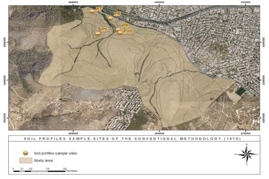
Figure 2.
Soil profiles sample sites of the conventional soil mapping method.
The second mapping of the study area was carried out in 2019 according to the currently used soil mapping system following the physiographic methodology. In the context of the new soil mapping system, the preliminary delineation of SMUs was achieved by incorporating three digitized backgrounds in the GIS software, those of topography (GMS map at scale 1:50,000), geology [24] and the geometrically corrected ortho-photo map of the interested area from the Greek Cadaster (2007) as the main cartographic background at the scale 1:30,000. Finalization of SMUs boundaries was achieved by complementary on-site visual observations in the field in order to confirm or correct the initial delineated SMUs boundaries, using the Collector for ArcGIS software. Taking into consideration that the laboratory soil sampling analyses as well as the descriptions of the lowlands soil profiles of the 1976 study remained unchanged, they were used in the new mapping system to confirm the delineated SMUs of the lower parts of the Garden and to verify the corresponding taxonomical soil units. Based on the mapping scale and the size of the mapped area twelve soil sampling sites were selected and two soil samples were taken for laboratory analyses from the surface and subsurface horizons or layers of each sampling site, where possible (Figure 3).
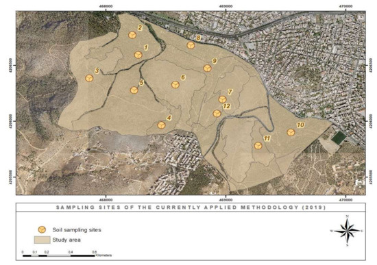
Figure 3.
Soil sampling sites of the currently applied mapping method.
The obtained results from the soil sample analyses, along with field measurements and observations, were used to confirm delineations and mapping symbols of SMUs of the 2019 and 1976 mapping methodologies. In order to also cover the hilly areas of the DBG and to increase the number of observations four (4) additional profiles were prepared and described in detail in existing soil cuts confirming the delineations and classifications of both methods (Figure 4 and Figure 5). The data were finally introduced in a specific geodatabase, in the ArcGIS v.10.4 environment.
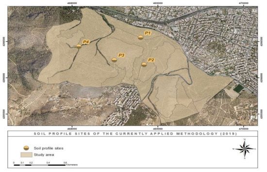
Figure 4.
Profile sites of the new soil mapping method.

Figure 5.
Representative soil profiles described in 2019: (a) Cambisol formed on limestone parent material with calcic horizon (Profile P1), (b) Cambisol formed on limestone parent material with a petrocalcic horizon at the depth >80 cm (Profile P2), (c) Cambisol formed on limestone parent material rich in rock fragments (Profile P3), (d) Leptosol formed on limestone parent material with bedrock at depth ≥ 20 cm (Profile P4).
2.4. Comparison of the Results of the Two Methodologies
The comparison of the two methodologies was made on the basis of the spatial coincidence between the two classification systems and the successful or not common description of the soils achieved via the two cartographic symbols. Specifically, with the use of geospatial techniques, in the ArcGIS v.10.4. environment, the eight taxonomic categories of the 2019 mapping system were used as clipping surfaces for the extraction of the 1976 SMUs that spatially coincided with them. Subsequently, the spatial correspondences between each taxonomic category of the 2019 mapping, that was used as the base reference for the analysis and the taxonomic categories of the 1976 SMUs were emerged. Then, an analysis of the participation rates (%) of the 1976 SMUs areas that presented the same classification with each taxonomic category of the 2019 mapping was performed inside the eight clipped common areas (Section 4.2, Appendix B, Table A11). Based on the areas, resulted from the participation rates and grossed up to the total area of each taxonomic category of 2019 mapping, the percentages of agreement between the classifications of the two methods were calculated (Section 4.2, Appendix B, Table A12). The overall percentage of taxonomic coincidence between the two systems, presented in conclusions (Section 5), emerged as the average of the individual percentages of agreement (Figure 6), (Appendix B, Table A12). Afterwards, the properties of the cartographic symbols of the two methodologies were compared in order to evaluate the description of the soils achieved by the two systems. Regarding the comparison of the two cartographic symbols, it was considered that the area corresponded to each taxonomic category of 2019, multiplied by its individual percentage of agreement with the 1976 classification, defined the new area for the comparison of the two symbols concerning all of the other soil properties except classification as it was already being evaluated. Then, depending on whether it was observed inside the spatial boundaries of the eight new areas a coincidence or not of the soil properties of the two symbols greater than 80% based on the participation rates, explained previously, the areas corresponding to a common description of soil properties (except classification) between the two systems were calculated. These areas were considered as the rates of success for the common description of the soils by the symbols of the two methods. The overall percentage (Section 5) of success for the common description of the soils by the mapping symbols of the two systems, presented in conclusions (Section 5), emerged as the summation of the individual success rates respectively, grossed up to the total area of DBG (Figure 6), (Appendix B, Table A12).
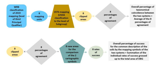
Figure 6.
Schematic presentation showing the procedures for comparison of the two mapping systems. The spatial object of WRB classification fragmented into 8 mapping units according to the 8 taxonomical categories. The 8 mapping units also included all the information of the cartographic symbol of 2019 mapping. Each mapping unit was used as a clipping surface for the extraction of SMUs of 1976 mapping that contained all the information of the cartographic symbol of 1976 mapping including the USDA classification.
3. Results
3.1. Soil Map and Soil Groups Derived by the Conventional Mapping System
According to the 1976 soil mapping, fifty-five (55) SMUs were identified [32], delineated and described in the scale of 1:5,000 (Figure 7, Appendix A-A1, Table A1, Appendix B, Table A8). The main identified soil order was Entisols covering 111.9 ha or 64.1% of the mapped area, while the next important soil order was Inceptisols covering 62.7 ha or the 35.9% of the study area. The subgroup of Lithic Xerorthents prevailed in Entisols covering 110 ha or the 98.3% of these soils. A small area of 1.1 ha or 1.0% of Entisols were characterized as Typic Xerofluvents. In addition, Typic Xerorthents also covered a small area of 0.8 ha or the 0.7% of Entisols (Table 1., Figure 8). Typic Xerofluvents included mainly deep, calcaric and medium textured allochthonous soils formed on Holocene alluviums characterized by a xeric soil moisture regime and located in the lower part of the DBG. Typic or Lithic Xerorthents are located in the hilly part of DBG, strongly sloping, formed mainly on limestone parent material. These two Subgroups of Xerorthents are distinguished by the presence or not of a lithic contact within 50 cm of the mineral soil surface. In Inceptisols the majority of the mapped soils were characterized as Typic Calcixerepts (54.7 ha or the 87.2% of Inceptisols) while Petrocalcic Calcixerepts covered 8 ha or the 12.8% of these soils. Typic Calcixerepts were soils mainly freely drained with presence of a calcic horizon within 100 cm of the mineral soil surface, while Petrocalcic Calcixerepts were characterized by a petrocalcic horizon within 100 cm of the mineral soil surface (Figure 8).
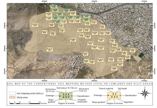
Figure 7.
Soil Mapping Units (SMUs) delineations and mapping symbols according to the conventional mapping methodology (1976).

Table 1.
Grouping of soils according to the United States Department of Agriculture (USDA) taxonomical system to the level of Subgroup.
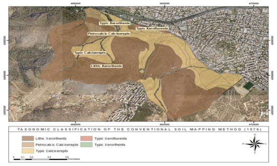
Figure 8.
Soil taxonomic units (Subgroups) according to the conventional mapping methodology (1976).
3.2. Soil Map and Soil Groups Derived From the Currently Applied (2019) Mapping Methodology
In the context of the 2019 mapping system, nineteen (19) SMUs were emerged, delineated and described in the scale of 1:30,000 (Figure 9, Appendix A and Appendix A.1., Table A1, Appendix B, Table A9). The prevailing RSG was Leptosols covering 106.9 ha or 61.4% of the area, while 52.3 ha were identified as Cambisols corresponding to 30.1% of the mapped area. Calcisols occupied a small part of the DBG covering 14.7 ha or 8.5% of the studied area. Calcaric Skeletic Nudilithic Leptosols (LP-nt.sk.ca) [1] were the major soil group of Leptosols covering 38.1 ha or 35.6% of the RSGs followed by Skeletic Calcaric Cambic Leptosols (LP-cm.ca.sk) occupying an area of 25.7 ha or 24.1% of the RSG. Skeletic Calcaric Nudilithic Leptosols (LP-nt.ca.sk) and Cambic Calcaric Skeletic Leptosols (LP-sk.ca.cm) shared almost the same percentages (20.4% and 19.9%) of Leptosols covering 21.8 and 21.3 ha respectively. LP-nt.sk.ca were shallow soils (depth ≤ 25 cm) primarily with bedrock exposed on the soil surface, having 40% (by volume) rock fragments and evidences of calcaric material. LP-cm.ca.sk characterized as shallow soils (depth ≤ 25 cm) primarily having a cambic horizon (thickness ≥ 15 cm) with evidences of calcaric material and presenting 40% (by volume) rock fragments. LP-nt.ca.sk were also shallow soils (depth ≤ 25 cm) with bedrock partially exposed on the soil surface having evidences of calcaric material as well as a considerable amount of rock fragments 40% (by volume). LP-sk.ca.cm were shallow soils (depth ≤ 25 cm) primarily presenting 40% (by volume) rock fragments and also having evidence of calcaric material and a cambic horizon (thickness ≥ 15 cm). As far as Cambisols is concerned, Leptic Skeletic Calcaric Cambisols (CM-ca.sk.le) were the most significant group mapped covering 25.2 ha or the 48.2% of the RSG. The second most important soil group of Cambisols was Skeletic Calcaric Leptic Cambisols (CM-le.ca.sk) covering 18.6 ha or 35.5% of this area. Chromic Leptic Calcaric Cambisols (CM-ca.le.cr) occupied 8.5 ha or 16.3% of Cambisols. Calcisols were grouped as Skeletic Cambic Petric Calcisols (CL-pt.cm.sk) covering only 14.7 ha (Table 2., Figure 10). CM-ca.sk.le were soils with a cambic horizon (thickness ≥ 15 cm) mainly presenting evidence of calcaric material, 40% (by volume) rock fragments and bedrock at a depth ≤ 100 cm from the soil surface. CM-le.ca.sk were soils with a cambic horizon (thickness ≥ 15 cm) mainly with bedrock at a depth ≤ 100 cm from the soil surface, having also evidences of calcaric material and an amount of 40% (by volume) rock fragments. CM-ca.le.cr were soils with a cambic horizon (thickness ≥ 15 cm) mainly with evidences of calcaric material having bedrock at a depth ≤ 100 cm from the soil surface and a layer between 25 and 150 cm from the soil surface (thickness ≥ 30 cm) having a Munsell color hue redder than 7.5 YR. CL-pt.cm.sk included soils with a calcic or petrocalcic horizon at a depth ≤ 100 cm from the soil surface mainly presenting a cemented or indurated layer starting at a depth ≤ 100 cm from the soil surface, evidences of a cambic horizon (thickness ≥ 15 cm) and 40% (by volume) rock fragments (Figure 10). Fluvisols were not possible to map, whereas Fluvents were found in the conventional method, because the MLA of the currently applied methodology (due to the scale of 1:30,000) was 3.6 ha and Fluvents covered an area of 1.1 ha.
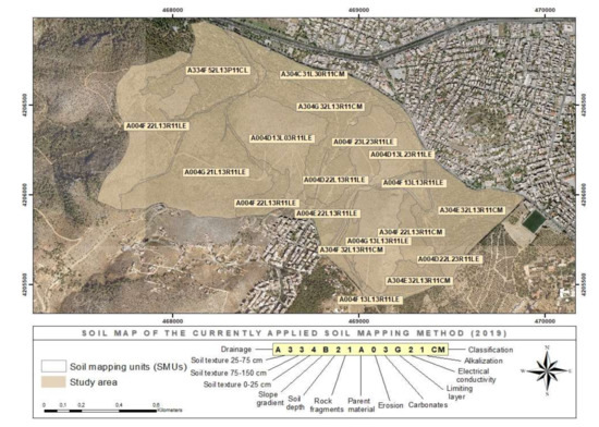
Figure 9.
SMUs delineations and mapping symbols according to the currently applied methodology (2019).
Table 2.
Grouping of soils according to the World Reference Base for Soil Resources (WRB) taxonomical system to the level of third Principal Qualifier.
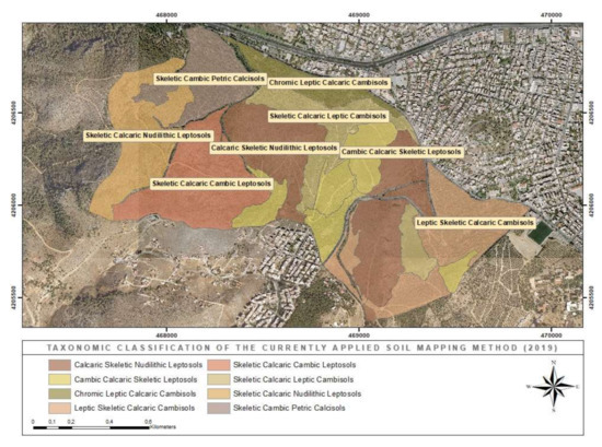
Figure 10.
World Reference Base for Soil Resources (WRB) soil classification according to the currently applied mapping methodology.
4. Discussion
As it was highlighted above, the numerical alteration between the fifty-five (55) and the nineteen (19) SMUs of the conventional (old) and the current (new) soil mapping system, respectively, was attributed to the different used scale of the two methodologies. As it had been thoroughly reported in the case of the present work, the delineation of 1976 was mainly conducted on a detailed topographical background of 1:5,000 scale under a detailed SMU delineation method, while the delineation of 2019 was mainly conducted on semi-detailed ortho-imagery backgrounds of 1:30,000, under a semi-detailed SMU delineation methodology.
4.1. Data Provided by the Two Soil Mapping Systems
In the Appendix A (Table A1) the soil properties with the corresponding classes of the two mapping symbols used by the conventional (1976) and currently applied (2019) systems are shown. The two symbols and thus the two soil mapping systems recorded and transferred largely the same amount of soil information since nine (9) of the fifteen (15) mapped soil properties were common between the two systems (an example of a common soil property is given in Figure 11 and Figure 12). The soil classification was identified by using different taxonomical systems in the two mapping systems (USDA and WRB) but as it will be discussed, the two classification systems were largely compatible concerning the types of soil information recorded per taxonomic category. The cartographic symbol of the conventional method included one (1) additional property concerning the prevailing type of vegetation. The cartographic symbol of the new method included an additional set of five (5) soil properties, over that of the old method, related to soil depth, presence of rock fragments (gravels and cobbles) on the soil surface, limiting layers, electrical conductivity and alkalization. All the above-mentioned additional properties are of great value for agricultural production and soil protection. Soil depth can be extracted inductively and indirectly from the texture of the three soil layers of the lowlands old mapping symbol up to a depth of 150 cm. However, it is very important the soil depth to be measured more accurate due to its great importance on soil water storage capacity and plant growth. Parent material was presented in the mapping symbol of the conventional system only for hilly soils. However, parent material is a significant soil parameter even in transported allochthonous lowland soils affecting chemical and physical properties. For example, soils formed on recent alluvial deposits are usually more fertile compared to soils formed on alluvial terraces. Additionally, the percentage of rock fragments in the soil surface affects soil moisture conservation and soil erosion susceptibility [40]. The conventional mapping system for the alluvial soils (lowlands) recorded the presence of gravels in the three textural layers, depending on the depth that they were observed (Appendix A, Table A1 and Appendix B, Table A8). In fact, gravels affect effective soil water storage capacity and rooting depth considered this recording as an advantage in relation to the new mapping system. The type and the kind of a limiting layer is an important property to be recorded affecting soil water movement and penetration of plant roots. Finally, electrical conductivity and alkalization are key soil parameters especially for the characterization of the salt-affected soils of the lowlands and coastal areas. In conclusion, the new mapping symbol can be considered as an effort of unifying the two symbols used to cover the plain and hilly soils according to the conventional mapping under one mapping symbol. Additionally, the new mapping symbol included more soil characteristics, easily identified in the field, of great importance for plant growth and soil protection. The use of one mapping system for all soils gives the opportunity to the user of having a uniform soil database independently of the origin of the soils.
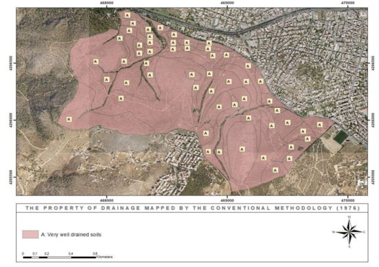
Figure 11.
Drainage map of the conventional mapping system.
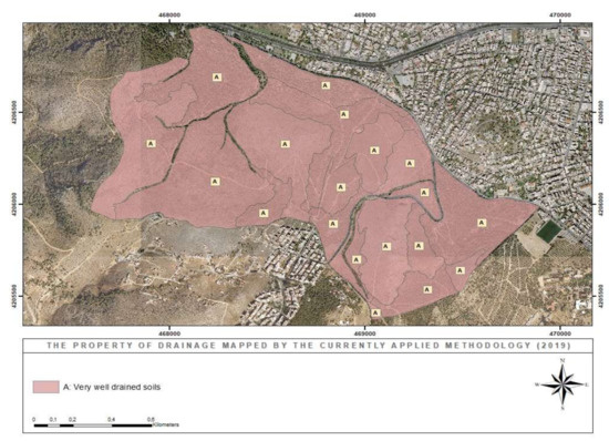
Figure 12.
Drainage map of the currently applied mapping system.
4.2. Reliability and Compatibility of the wo Mapping Systems
According to USDA [39] and WRB [37] soil taxonomical systems it was evident that there was an identification between the general taxonomical classes of Order and Reference Soil Group (RSG) as far as Inceptisols and Cambisols were concerned. Regarding the Order of Entisols on the basis of the previously mentioned taxonomical systems they can only partially agree with the RSGs of Leptosols and Fluvisols.
Based on the results of the present work, Skeletic Calcaric Nudilithic Leptosols (SMU 18 from the 2019 mapping including 82% of SMU 11 and 41% of SMU 12 of the 1976 mapping) corresponded to Lithic Xerorthents in 93.6% of their area, highlighting an excellent agreement between the classifications of the two systems (Table 3). In addition, the remaining soil parameters of the cartographic symbols of SMUs of both mapping systems were largely coincided and characterized the soils mainly as shallow, freely drained, strongly inclined, formed on limestone and subjected to none or weak erosion (Appendix B, Table A10). The other 6.4% of Skeletic Calcaric Nudilithic Leptosols corresponded to Typic Calcixerepts in 1976 mapping (SMU 18 from the 2019 mapping including 100% of SMU 43). However, apart from the negligible mismatch in classification the soils of this group were similarly characterized by the two methodologies as very well drained, shallow, strongly inclined, formed on limestone and subjected to none or weak erosion (Appendix B, Table A10).
Table 3.
Table of differences between the classifications of the two systems on a spatial basis.
Calcaric Skeletic Nudilithic Leptosols (SMUs 2,4,6,11,16 from the 2019 mapping including 43% of SMU 13, 92% of SMU 16, 12% of SMU 18, 65% of SMU 20, 100% of SMU 27,62% of SMU 31 of the 1976 mapping) characterized as Lithic Xerorthents in 75.9% of their area, noting a very good match between the two classification systems (Table 3). The recorded soil properties by the two mapping methods in this taxonomic group were largely coincided characterizing the soils mainly as shallow, freely drained, strongly inclined, formed on limestone and subjected to no or weak erosion (Appendix B, Table A10). The remaining 24.1% of Calcaric Skeletic Nudilithic Leptosols characterized as Typic Calcixerepts in 1976 mapping (SMUs 2,4,6,11,16 from the 2019 mapping including 48% of SMU 19, 15% of SMU 25, 52% of SMU 28, 42% of SMU 32, 68% of SMU 33, 31% of SMU 34, 43% of SMU 35, 97% of SMU 44, 100% of SMU 45, 30% of SMU 47) and recorded a small mismatch in the classification property. However, as far as the rest soil properties of this group are concerned the two mapping systems described the soils in a similar way mostly as very well drained, formed on limestone, moderately to strongly inclined and subjected to none or weak erosion (Appendix B, Table A10).
Cambic Calcaric Skeletic Leptosols (SMUs 1,8,9,12,17 from the 2019 mapping including 3.8% of SMU 12, 13% of SMU 13, 98% of SMU 26, 7% of SMU 29, 14% of SMU 30, 37% of SMU 31,90% of SMU 36, 100% of SMU 37, 29% of SMU 39, 82% of SMU 49 of the 1976 mapping) corresponded to Lithic Xerorthents in 75.6% of their area, presenting a very good match between the two classification systems (Table 3). The two soil mapping methods characterized the soils of the above-mentioned group partly in a similar manner mainly as very well drained, strongly inclined, formed on limestone and subjected to none or weak erosion. There were some discrepancies in parent material and soil depth in SMUs 13 and 26 of the 1976 mapping characterized the soils as deep and formed on shale. The majority of the soils of this group (1976 SMUs 30,31,36,39) according to the 1976 mapping were mainly recorded as deep in contradiction to the 2019 mapping method (Appendix B, Table A10). The remaining 24.4% to complete the class of Cambic Calcaric Skeletic Leptosols was characterized as Typic Calcixerepts in 1976 mapping (SMUs 1,8,9,12,17 from the 2019 mapping including 39% of SMU 14, 95% of SMU 15, 40% of SMU 32, 13% of SMU 34). However, there was a close match with the rest soil properties between the two systems that characterized the soils of this group as shallow, very well drained, moderately to strongly inclined, formed on limestone and subjected to none or weak erosion (Appendix B, Table A10).
Skeletic Calcaric Cambic Leptosols (SMU 19 from the 2019 mapping including 54% of SMU 12 and 38% of SMU 13 of the 1976 mapping) characterized as Lithic Xerorthents in 73.2% of their area and showed a very good match between the two classification methods (Table 3). The soil properties mapped by the two methods for these soils were not similar because of the discrepancies of 1976 SMU 13 that characterized the soils mainly as deep and formed on shale (Appendix B, Table A10). The rest 26.8% of Skeletic Calcaric Cambic Leptosols corresponded to Typic Calcixerepts in 1976 mapping (SMU 19 from the 2019 mapping including 100% of SMU 51) and noted a mismatch in the classification and in basic soils properties between the two systems since 1976 classification characterized soils of this group mainly as deep and strongly inclined (Appendix B, Table A10).
Chromic Leptic Calcaric Cambisols (SMU13 from the 2019 mapping including 13% of SMU 34, 79% of SMU 40, 76% of SMU 41, 38% of SMU 42, 98% of SMU 46, 5% of SMU 47, 97% of SMU 50, 55% of SMU 53 of the 1976 mapping) matched in 65.0% of their area to Typic Calcixerepts, demonstrating a good agreement of the two classification systems (Table 3). The majority of these soils had the same characteristics between the two mapping methods recorded mainly as deep, moderately fine textured in the surface layer (0–25 cm), very well drained, slightly or moderately inclined with strong reaction on the soil surface (Appendix B, Table A10). The remaining 35% of Chromic Leptic Calcaric Cambisols was differentiated into three taxonomic categories of 1976 mapping those of Typic Xerorthents (SMU 13 from the 2019 mapping including 100% of SMU 55), Lithic Xerorthents (SMU 13 from the 2019 mapping including 100% of SMU 54) and Typic Xerofluvents (SMU 13 from the 2019 mapping including 100% of SMU 52). Although the taxonomic class of 2019 mapping was divided into 3 classes in 1976 mapping, it was observed a great overlap in the description of the soils of this group which were mainly characterized as deep, very well drained, slightly or moderately inclined, with strong reaction on the soil surface and subjected to none or weak erosion soils (Appendix B, Table A10).
Skeletic Cambic Petric Calcisols (SMU 15 from the 2019 mapping including 98% of SMU 1, 100% of SMU 2, 100% of SMU 4, 100% of SMU 6, 100% of SMU 7, 100% of SMU 8, 100% of SMU 10, 100% of SMU 48 of the 1976 mapping) characterized as Typic and Petrocalcic Calcixerepts in 60% of their area, presenting a moderate good match between the classifications of the two systems (Table 3). Over one half of Typic and Petrocalcic Calcixerepts classes (1976 SMUs 1,2,4,6,48) corresponding to the lowland’s mapping system, were mostly characterized as very well drained soils, moderately fine textured in the surface layer (0–25 cm), inclined, with strong reaction on the soil surface and subjected to none or weak erosion as Skeletic Cambic Petric Calcisols (Appendix B, Table A10). The rest of the Typic and Petrocalcic Calcixerepts class (1976 SMUs 7,8,10) presented the same soil characteristics as Skeletic Cambic Petric Calcisols except soil texture, which did not appear on the mapping symbol because they were mapped as hilly soils. The remaining 40% of Skeletic Cambic Petric Calcisols corresponded to Lithic Xerorthents (SMU 15 from the 2019 mapping including 100% of SMU 3, 100% of SMU 5, 100% of SMU 9, 18% of SMU 11). However, apart from the considerable mismatch in classification the soils of this group were similarly characterized by the two methodologies mainly as deep, very well drained, strongly inclined, formed on limestone, with strong reaction on the soil surface and subjected to none or weak erosion (Appendix B, Table A10).
Leptic Skeletic Calcaric Cambisols (SMUs 3,5,7 from the 2019 mapping including 55% of SMU 14, 93% of SMU 17, 46% of SMU 19, 98% of SMU 21, 98% of SMU 22, 97% of SMU 23, 97% of SMU 24, 82% of SMU 25, 56% of SMU 35 of the 1976 mapping) corresponded to Typic Calcixerepts in 58% of their area indicating a moderate good match between the classifications of the two methodologies (Table 3). The two mapping methodologies had also the same results as far as soil parameters of the mapping symbols are concerned and characterized the soils mainly as deep, very well drained, moderately to strongly inclined, formed on limestone and subjected to none or weak erosion, except of a minor mismatch of SMU 24 that characterized the soils as deep and formed on shale (Appendix B, Table A10). The remaining 42% of Leptic Skeletic Calcaric Cambisols corresponded to Lithic Xerorthents (SMUs 3,5,7 from the 2019 mapping including 59% of SMU 18, 14% of SMU 20, 86% of SMU 29, 80% of SMU 30, 18% of SMU 49). This soil group had a moderate mismatch in classification but regarding the soil properties of the mapping symbols of the two methods the results were similar and the soils were characterized mainly as very well drained, moderately deep or deep, strongly inclined, formed on limestone and subjected to none or weak erosion (Appendix B, Table A10).
Skeletic Calcaric Leptic Cambisols (SMUs 10,14 from the 2019 mapping including 48% of SMU 28, 18% of SMU 32, 30% of SMU 33, 44% of SMU 34, 97% of SMU 38, 19% of SMU 40, 24% of SMU 41, 63% of SMU 42, 3% of SMU 44, 64% of SMU 47, 45% of SMU 53 of the 1976 mapping) characterized as Typic Calcixerepts in 55.0% of their area, presenting a moderate to good agreement between the classifications of the two methodologies (Table 3) and a good match between the soil properties of the two different mapping symbols that characterized the soils mainly as freely drained, deep, strongly inclined and subjected to none or weak erosion (Appendix B, Table A10). The other 45.0% of the Skeletic Calcaric Leptic Cambisols area was characterized as Lithic Xerorthents (SMUs 10,14 from the 2019 mapping including 7% of SMU 13, 7% of SMU 16, 28% of SMU 18, 19% of SMU 20, 4% of SMU 29, 5% of SMU 30, 10% of SMU 36, 71% of SMU 39) and a moderate mismatch was noted in the classification property and a moderate mismatch in soil depth and parent material since SMU 13 was differentiated from 2019 mapping characterized the soils as deep and formed on shale parent material (Appendix B, Table A10).
5. Conclusions
Our study showed that the conventional mapping system was based on more detailed mapping backgrounds and thorough crossings within the SMUs for their delineation. Following the conventional soil mapping system, the delineated SMUs were smaller and more detailed than the SMUs of the currently applied mapping system. Due to the technological shortcomings of that time and the absence of a global or national geodetic reference system, the detailed delineations of SMUs of the conventional system could not be placed in their exact positions due to errors generated during spatial information transferring from the digitized and uncorrected old map grids to georeferenced backgrounds in modern reference systems.
The comparison of the cartographic symbols of the two mapping systems (conventional and currently applied) showed that the two mapping symbols convey a common critical mass of information since nine over fifteen properties are common between them (Section 4.1.). However, the conventional soil mapping system have used two cartographic symbols one for the hilly residual soils and one for the lowland alluvial soils with the risk of creating confusion in organizing a database. In the opposite, in the currently applied soil mapping system, one cartographic symbol was been assigned for both hilly residual soils and lowland alluvial soils providing the advantage of an easily established database. (Section 4.1.). A major weakness of the new mapping symbol is that two soil parameters, namely electrical conductivity and alkalization, require measurement in the field with scientific instruments or laboratory soil analysis. This disadvantage differentiates the new symbol from the general philosophy of creating soil cartographic symbols using parameters easily recognizable in the field.
The comparison of the taxonomic systems (WRB and USDA) of the two mapping methodologies have shown an average coincidence of 69.5% (Section 4.2., Appendix B, Table A12). Regarding the descriptions of the soils (except classification) based on the cartographic symbols of the two methodologies (conventional and currently applied), the percentage of agreement between the two methods reached 63.7% (Section 4.2., Appendix B, Table A12).
According to the results of this work, the two mapping systems (conventional and currently applied) can be creatively combined and can function complementary to each other for a better mapping of soils. In many cases the more detailed but uncorrected SMUs of the conventional mapping could be used to highlight some important areas of specific agricultural management within the coarser and georeferenced SMUs of the currently applied mapping system. Considering that the main soil information recorded by the two systems is common, the two cartographic symbols could be combined satisfactory for a more detailed and accurate description of soil parameters.
We finally consider the results of this work as a starting point in an effort of utilizing and integrating the existing old soil mapping data in the national soil map of Greece. Of course, towards to this direction several other assessments of the compatibility of the two systems, especially in extended and lowland agricultural areas, should follow given that our work has been limited mainly to hilly forest soils of a small area. At a country level, given that this effort will be massive and laborious, it is very important to be supported as much as possible with the products and techniques of DSM [7,8]. In the present study, digital mapping was not used supportively because the subject was the comparison of two classical soil mapping methods and the study area was restricted.
Author Contributions
Conceptualization, O.K., C.K. and N.M.; methodology, O.K., N.Y., C.K. and N.M.; software, O.K. and V.D.; field supervision, C.K. and N.M. data analysis, O.K., V.D. and C.A.; writing—original draft preparation, O.K., V.D. and C.A.; writing—review and editing, O.K., D.G., C.K. and N.M. All authors have read and agreed to the published version of the manuscript.
Funding
This research received no external funding.
Acknowledgments
The authors must acknowledge and thank Soulios Stelios who allowed all the necessary field work for soil mapping in Diomedes Botanical Garden to be carried out appropriately.
Conflicts of Interest
The authors declare no conflict of interest.
Abbreviations
| AUA | Agricultural University of Athens |
| DBG | Diomedes Botanical Garden |
| DSM | Digital Soil Mapping |
| ESRI | Environmental Systems Research Institute |
| FAO | Food and Agriculture Organization of the United Nations |
| GGRS87 | Greek Geodetic Reference System 87 |
| GIS | Geographic Information System |
| MLA | Minimum Legible Area |
| MLD | Minimum Legible Delineation |
| PQ | Principal Qualifier |
| RSG | Reference Soil Group |
| SMU | Soil Mapping Unit |
| STU | Soil Typological Unit |
| SQ | Supplementary Qualifier |
| USDA | United Stated Department of Agriculture |
| WRB | World Reference Base for Soil Resources |
Appendix A
Table A1.
Parameters of the conventional and currently applied soil mapping symbol and their corresponding classes.
Table A1.
Parameters of the conventional and currently applied soil mapping symbol and their corresponding classes.
| Parameters and Their Corresponding Classes | ||||||||||||||||||||||||||||||||||||||||
|---|---|---|---|---|---|---|---|---|---|---|---|---|---|---|---|---|---|---|---|---|---|---|---|---|---|---|---|---|---|---|---|---|---|---|---|---|---|---|---|---|
| Drainage conditions * | ||||||||||||||||||||||||||||||||||||||||
| Very well drained soils (>150 cm) | Well drained soils 100–150 cm | Moderately well drained soils 50–100 cm | Imperfectly drained soils 30–50 cm | Poorly drained soils < 30 cm | Very poorly drained soils F Gley (75–150 cm), G Gley < 75 cm | |||||||||||||||||||||||||||||||||||
| A | B | C | D | E | F | G | ||||||||||||||||||||||||||||||||||
| Soil texture (0–25 cm) *,1,2 | ||||||||||||||||||||||||||||||||||||||||
| Very coarse (S, LS) | Coarse (SL) | Medium (L, SiL, Si) | Moderately fine (CL, SCL, SICL) | Fine (C, SC, SiC) | ||||||||||||||||||||||||||||||||||||
| 1 | 2 | 3 | 4 | 5 | ||||||||||||||||||||||||||||||||||||
| Soil texture (25–75 cm) *,1,2 | ||||||||||||||||||||||||||||||||||||||||
| Very coarse, coarse (S, LS, SL) | Medium (L, SiL, Si) | Moderately fine (CL, SCL, SICL) | Fine (C, SC, SiC) | |||||||||||||||||||||||||||||||||||||
| 1 | 2 | 3 | 4 | |||||||||||||||||||||||||||||||||||||
| Soil texture (75–150 cm) *,1,2 | ||||||||||||||||||||||||||||||||||||||||
| Very coarse, coarse (S, LS, SL) | Medium (L, SiL, Si) | Moderately fine (CL, SCL, SiCL), fine C, SC, SiC) | ||||||||||||||||||||||||||||||||||||||
| 1 | 2 | 3 | ||||||||||||||||||||||||||||||||||||||
| Soil depth (cm) * | ||||||||||||||||||||||||||||||||||||||||
| 0–15 | 15–30 | 30–60 | 60–100 | 100–150 | >150 | |||||||||||||||||||||||||||||||||||
| 1 | 2 | 3 | 4 | 5 | 6 | |||||||||||||||||||||||||||||||||||
| Slope gradient (%) * | ||||||||||||||||||||||||||||||||||||||||
| 0–2 | 2–6 | 6–12 | 12–18 | 18–25 | 25–35 | >35 | ||||||||||||||||||||||||||||||||||
| A | B | C | D | E | F | G | ||||||||||||||||||||||||||||||||||
| Rock fragments (%) ** | ||||||||||||||||||||||||||||||||||||||||
| <20 | 20–60 | >60 | ||||||||||||||||||||||||||||||||||||||
| 1 | 2 | 3 | ||||||||||||||||||||||||||||||||||||||
| Parent material * | ||||||||||||||||||||||||||||||||||||||||
| Marl | Conglomerates | Limestone, marbles | Alluvial deposits | Schist | Flysch | |||||||||||||||||||||||||||||||||||
| M | C | L | A | S | P | |||||||||||||||||||||||||||||||||||
| Acid igneous | Basic igneous | Clay deposits | Volcanic ash | Magmatic conglomerates | Alluvial fan | |||||||||||||||||||||||||||||||||||
| O | Β | G | H | K | R | |||||||||||||||||||||||||||||||||||
| Lake deposits | Sand dunes | Organic deposits | Alluvial terraces | Sandstone | ||||||||||||||||||||||||||||||||||||
| Y | D | X | T | I | ||||||||||||||||||||||||||||||||||||
| Inorganic carbonates * | ||||||||||||||||||||||||||||||||||||||||
| Strong reaction on the soil surface | Weak reaction on the soil surface | Reaction in the subsurface horizon or in substratum | No reaction | |||||||||||||||||||||||||||||||||||||
| 3 | 2 | 1 | 0 | |||||||||||||||||||||||||||||||||||||
| Degree of erosion * | ||||||||||||||||||||||||||||||||||||||||
| No erosion | Weak erosion (< 25% A horizon) | Moderate erosion (25–75% A horizon) | Severe erosion (no A horizon) | Very severe erosion (gullies) | ||||||||||||||||||||||||||||||||||||
| 0 | 1 | 2 | 3 | 4 | ||||||||||||||||||||||||||||||||||||
| Limiting Layers ** | ||||||||||||||||||||||||||||||||||||||||
| No | Bedrock | Gravels or sand | Compact horizon | |||||||||||||||||||||||||||||||||||||
| 0 | R | G | F4 | |||||||||||||||||||||||||||||||||||||
| Electrical conductivity (dS/m) ** | ||||||||||||||||||||||||||||||||||||||||
| 0–4 | 4–8 | 8–15 | >15 | |||||||||||||||||||||||||||||||||||||
| 1 | 2 | 3 | 4 | |||||||||||||||||||||||||||||||||||||
| Alkalization (Exchangeable Sodium Percentage—ESP) ** | ||||||||||||||||||||||||||||||||||||||||
| ESP < 6 | ESP = 6.1–15 | ESP > 15 | ||||||||||||||||||||||||||||||||||||||
| 1 | 2 | 3 | ||||||||||||||||||||||||||||||||||||||
| Soil classification (WRB) | ||||||||||||||||||||||||||||||||||||||||
| Cambisols | Calcisols | Regosols | Fluvisols | Luvisols | Leptosols | |||||||||||||||||||||||||||||||||||
| CM | CL | RG | FL | LV | LP | |||||||||||||||||||||||||||||||||||
| Soil classification (USDA) | ||||||||||||||||||||||||||||||||||||||||
| Entisols | Inceptisols | Alfisols | Histosols | |||||||||||||||||||||||||||||||||||||
| E | I | A | Hs | |||||||||||||||||||||||||||||||||||||
*—Common properties of conventional and currently applied mapping symbols; **—Additional properties of currently applied mapping symbol; 1—In soil texture symbols of the three textural layers of the alluvial soils, according to the conventional method, the presence of gravels was recorded depending on the depth that they were observed by noting their presence with the symbol x (>60%) or o (<60%) as exponents above the number denoting the texture of each depth; 2—In cases where there is no soil in a particular layer the symbol 0 is assigned.
Appendix A.1. Guidelines for the Characterization of the Soil Properties Used in the Conventional and Currently Applied Soil Mapping Symbols
Drainage Conditions
The characterization of the drainage conditions is based on the presence of iron or manganese mottles and the subsoil colorings. The six (6) hydromorphic classes which are used in the soil mapping system are the following:
Class A—Very well drained soils
They are characterized by the absence of iron and manganese mottles throughout the whole soil profile. The brownish colors prevail, the soil usually has a high hydraulic conductivity and the water is infiltrated into the soil’s deepest layers. The soil remains wet only during the wet period of the year (wet months). Drainage is not required.
Class B—Well drained soils
They are characterized by the presence of iron and manganese mottles or gray mottles at a depth between 100 and 150 cm from the soil surface. The brown colors prevail throughout the whole soil profile. During the growing season, these soils are not sufficiently wet for a long period of time to adversely affect the growth of the plants. Drainage is not required.
Class C—Moderately well drained soils
They are characterized by the presence of iron and manganese mottles or gray mottles at a depth between 50 and 100 cm from the soil surface. In some soils of this class, there may be mottles at depths of less than 50 cm but its percentage is less than 2%. The underground aquifer in the wet months rises and may adversely affect perennial crops. These soils require drainage for sensitive crops.
Class D—Imperfectly drained soils
They are characterized by the presence of iron and manganese mottles or some reductive spots at a depth between 30 and 50 cm from the soil surface. The percentage of mottles in this layer is less than 20%. These soils are characterized by high moisture for a long period of the year close to the soil surface, resulting adverse consequences to the cultivations during the spring. Drainage is required for the perennial crops.
Class E—Poorly drained soils
They are characterized by the presence of iron and manganese mottles at a depth less than 30 cm from the soil surface while the presence of iron and manganese mottles or reductive spots covers a percentage of 20–50% at a depth between 30 and 50 cm from the soil surface. These soils have a high level of ground water table during the wet months of the year. The cultivation of perennial crops or early spring crops requires drainage.
Class F, G—Very poorly drained soils
Soils with a permanent ground water table at a depth commonly higher than 75 cm from the soil surface. If reducing conditions prevail at a percentage higher than 50 % at the depth of 75–150 cm, the soil is characterized by F drainage class. If the reductive conditions prevail at a depth less than 75 cm, the soil is characterized by G drainage class. If there is a seasonal fluctuation of the aquifer, the drainage class may be characterized by combining two of the previous classes (e.g., E/F, E/G andso forth). These soils are wet to the surface for the longest period of the year and therefore prevent the normal growth of most cultivations. Drainage is absolutely required.
Soil Texture
The soil texture is determining in the field using the sense of touch. The soil sample is moistened between the fingers index and thumb and the soil aggregates are broken due to the pressure and friction applied to the soil. The class of soil texture is determined accordingly to the sense of sticking (clay), gliding (silt) or gritting (sand). Soils that have a high percentage of sand have a gritty sense. Soils that have a high percentage of silt feel smooth while soils that have a high percentage of clay have a sticky feel. The corresponding symbols and sub-classes of soil texture are shown in Table A2.
Table A2.
Classes of soil texture with the corresponding symbols for the three parts of soil profile.
Table A2.
Classes of soil texture with the corresponding symbols for the three parts of soil profile.
| Map Symbol | Part A (0–25 cm) | Part Β (25–75 cm) | Part C (75–150 cm) |
|---|---|---|---|
| 1 | Coarse-textured or layers with predominant coarse-textured materials | Coarse-textured, moderately coarse-textured or predominant coarse-textured materials | Coarse-textured, moderately coarse-textured or predominant coarse-textured materials |
| 2 | Moderately coarse-textured or predominant moderately coarse-textured materials | Medium-textured or predominant medium-textured materials | Medium-textured or predominant medium-textured materials |
| 3 | Medium-textured or predominant medium-textured materials | Moderately fine-textured or predominant moderately fine-textured materials | Moderately fine-textured or predominant moderately fine-textured materials |
| 4 | Moderately fine-textured or predominant moderately fine-textured materials | Fine-textured or predominant fine-textured materials | |
| 5 | Fine-textured or predominant fine-textured materials | ||
| 6 | Muck | Muck | Muck |
| Coarse-textured | Sandy (S), Loamy-sand (LS) | ||
| Moderately coarse-textured | Sandy-loam (SL) | ||
| Medium-textured | Loamy (L), Silty-loam (SiL), Silty (Si) andfine Sandy-loam (fSL) | ||
| Moderately fine-textured | Sandy-Clay-Loam (SCL), Clay-Loam (CL) and Silty-Clay-Loam (SiCL) | ||
| Fine-textured | Silty-Clay (SiC), Clay(C) and Sandy-Clay (SC) | ||
Slope Gradient
The slope of the soil surface is determined on the field by the usage of a clysimeter, a topographical map or through estimation after acquisition of relevant experience. The slope gradient is distinguished in the following six (6) classes: almost flat (slope 0–2%), slightly inclined (slope 2–6%), moderately inclined (slope 6–12%), strongly inclined (slope 12–18%), moderately steep (slope 18 –25%), steep (slope 25–35%) and very steep (slope > 35%).
Rock Fragments
The content of rock fragments (gravels and cobbles) on the soil surface is estimated in the field using the classes which are shown in Table A3. Gravel is defined as the part of rock fragments with a diameter ranging from 2 mm to 7.5 cm. The cobbles include the rock fragments with a diameter > 7.5 cm.
Table A3.
Classes of rock fragments with the corresponding symbols.
Table A3.
Classes of rock fragments with the corresponding symbols.
| Map Symbol | Class Description |
|---|---|
| 1 | Gravels (diameter 2 mm–7.5 cm) and cobbles (diameter > 7.5 cm) on the soil surface in a percentage lower than 20 % |
| 2 | Gravels (diameter 2 mm–7.5 cm) and cobbles (diameter >7.5 cm) on the soil surface in a percentage ranging from 20 % to 40 % |
| 3 | Gravels (diameter 2 mm–7.5 cm) and cobbles (diameter > 7.5 cm) on the soil surface in a percentage higher than 60 % |
Parent Material
The parent material in each SMU is determined by field observations and the use of geological maps. As parent material is defined the upper geological layer on which the soil was formed. In each parent material a letter of the alphabet was given as shown in Table A1 (Appendix A).
Degree of Erosion
Erosion classes are defined by the presence or absence of diagnostic horizons and rills or gullies as follows (Table A4):
Table A4.
Erosion classes and their characteristics.
Table A4.
Erosion classes and their characteristics.
| Map Symbol | Class Description |
|---|---|
| 0 | No Erosion |
| 1 | Soils which have lost part of the surface horizon A but on average less than 25% of the initial horizon A. Indications for erosion class 1 are (a) few rills, (b) concentration of soil sediments at the base of the slope or in a cavity, (c) scattered spots where the horizon of cultivation contains materials from the underlying horizon. |
| 2 | Soils which have lost an average of 25–75% of the initial A horizon. In erosion class 2, the surface layer is consisted of a mixture of horizon A materials and the underlying subsurface horizon. In some areas there may be a mixed state of spots without any erosion signs and spots where all the A horizon has been removed. Where the horizon A is thick enough, minimum or no mixing of horizon A materials with materials of the underlying horizon has taken place. |
| 3 | Soils that have lost the whole A horizon and some of the deeper horizons to their greatest extent. The initial soil can be identified only on individual spots. |
| 4 | Soils that have lost the whole horizon A and some or all of the deeper horizons to their greatest extent. The initial soil can be identified only on individual spots. A complex system of rills and gullies is observed on the soil surface. |
Inorganic Carbonates
The inorganic carbonates are determined accordingly to their concentration and the depth where are detected indirectly by the reaction in dilute hydrochloric acid as follows (Table A5):
Table A5.
Classes of inorganic carbonates with the corresponding symbols.
Table A5.
Classes of inorganic carbonates with the corresponding symbols.
| Map Symbol | Class Description |
|---|---|
| 0 | No reaction throughout the whole soil profile |
| 1 | No reaction at the surface horizon of 0–30 cm (part A) while there is reaction at the subsurface horizon of 30–75 cm (part B) and/or at the substratum of 75–150 cm (part C). |
| 2 | Weak reaction on the surface horizon (part A) while the reaction at the deeper layers is not taken into account. |
| 3 | Strong reaction on the soil surface, while the reaction at the deeper layers is not taken into account. |
Limiting Layers
The presence of limiting layers that affects the growth of plant roots was observed through opening holes using soil-drills or in existing exposed soil profiles. As limiting layers are considered (a) solid rock, (b) cobbles or sand, (c) solid horizons impervious to water and roots such as a fragipan horizon. The corresponding symbols are given in Table A1 (Appendix A).
Electrical Conductivity
Electrical conductivity was recorded in the field according to the presence or absence of water-soluble salts and the formation on the soil surface of a white crust. The recording of the presence of salts or not was confirmed by laboratory measurement of the electrical conductivity of the soil. The following classes were distinguished 0–4 ds/m, 4–8 ds/m, 8–15 ds/m and> 15 ds/m with the corresponding symbols given in Table A1 (Appendix A).
Alkalization
The alkalization of the soil was determined according to the percentage of exchangeable sodium (ESP) and the cation exchange capacity. In alkaline soils, the amount of sodium retained by clay minerals is 15% or greater than the total cation exchange capacity (CEC). Alkalization was assessed based on previous soil studies and analyses. The used ESP classes were: ESP < 6, ESP = 6–15, ESP > 15% with the corresponding symbols given in Table A1 (Appendix A).
Soil Classification
The classification of the soils in the context of the two mapping methodologies (1976 and 2019) was carried out as described in the text of the present work based on the principles of USDA and WRB taxonomical keys.
Parent material of the hilly and mountainous soils
Table A6.
Soil mapping symbols for the hilly and mountainous areas according to the parent material.
Table A6.
Soil mapping symbols for the hilly and mountainous areas according to the parent material.
| Parent Material/Soil Depth (cm) | 0–30 | 30–100 | 100–150 | >150 |
|---|---|---|---|---|
| Granite | 01 | 02 | 03 | 04 |
| Limestone | 11 | 12 | 13 | 14 |
| Peridotite | 21 | 22 | 23 | 24 |
| Shale | 31 | 32 | 33 | 34 |
| Conglomerate Limestone Rock | 41 | 42 | 43 | 44 |
| Hornstone | 51 | 52 | 53 | 54 |
| Colluvial | 61 | 62 | 63 | 64 |
| Alluvial by diagenesis | 71 | 72 | 73 | 74 |
| Sandstone | 81 | 82 | 83 | 84 |
| Clayey Marls by diagenesis | 91 | 92 | 93 | 94 |
| Sandstone-Marls by diagenesis | 891 | 892 | 893 | 894 |
| Marls-Sandstone by diagenesis | 981 | 982 | 983 | 984 |
| Talc | 771 | 772 | 773 | 774 |
Vegetation type of the hilly and mountainous soils
Table A7.
Soil mapping symbols for the hilly and mountainous areas according to the type of vegetation.
Table A7.
Soil mapping symbols for the hilly and mountainous areas according to the type of vegetation.
| Symbol | Type of Vegetation |
|---|---|
| 0 | No vegetation |
| 1 | Shrubs |
| 2 | Not dense forests |
| 3 | Dense forests |
| 4 | Olives orchards |
| 5 | Vineyards |
Appendix B
Table A8.
SMU numbering, symbolization, occupied area and soil’s taxonomy of the conventional methodology (1976 mapping system).
Table A8.
SMU numbering, symbolization, occupied area and soil’s taxonomy of the conventional methodology (1976 mapping system).
| SMU_No | Conventional Soil Mapping Symbol | Order | Suborder | Great Group | Subgroup | Area (ha) |
|---|---|---|---|---|---|---|
| 1 | A3×04×I/C03 | Inceptisols | Xerepts | Calcixerepts | Petrocalcic | 1.3 |
| 2 | A304I/B03 | Inceptisols | Xerepts | Calcixerepts | Petrocalcic | 1.2 |
| 3 | A12E/F03 | Entisols | Orthents | Xerorthents | Lithic | 1.1 |
| 4 | A334I/C03 | Inceptisols | Xerepts | Calcixerepts | Petrocalcic | 0.4 |
| 5 | A12E/F03 | Entisols | Orthents | Xerorthents | Lithic | 1.3 |
| 6 | A203I/B03 | Inceptisols | Xerepts | Calcixerepts | Petrocalcic | 0.4 |
| 7 | A12I/B03 | Inceptisols | Xerepts | Calcixerepts | Petrocalcic | 0.8 |
| 8 | A12I/C03 | Inceptisols | Xerepts | Calcixerepts | Petrocalcic | 3.0 |
| 9 | A12E/F03 | Entisols | Orthents | Xerorthents | Lithic | 0.2 |
| 10 | A12I/E03 | Inceptisols | Xerepts | Calcixerepts | Petrocalcic | 0.9 |
| 11 | A11E/F02 | Entisols | Orthents | Xerorthents | Lithic | 17.6 |
| 12 | A11E/G01 | Entisols | Orthents | Xerorthents | Lithic | 14.7 |
| 13 | A34E/D00 | Entisols | Orthents | Xerorthents | Lithic | 28.7 |
| 14 | A12I/E03 | Inceptisols | Xerepts | Calcixerepts | Typic | 3.0 |
| 15 | A11I/E03 | Inceptisols | Xerepts | Calcixerepts | Typic | 2.3 |
| 16 | A11E/H01 | Entisols | Orthents | Xerorthents | Lithic | 10.6 |
| 17 | A12E/E03 | Inceptisols | Xerepts | Calcixerepts | Typic | 1.5 |
| 18 | A12E/F03 | Entisols | Orthents | Xerorthents | Lithic | 8.5 |
| 19 | A12I/E03 | Inceptisols | Xerepts | Calcixerepts | Typic | 2.0 |
| 20 | A11E/F02 | Entisols | Orthents | Xerorthents | Lithic | 4.9 |
| 21 | A41I/D02 | Inceptisols | Xerepts | Calcixerepts | Typic | 2.3 |
| 22 | A12I/D03 | Inceptisols | Xerepts | Calcixerepts | Typic | 0.6 |
| 23 | A42I/C02 | Inceptisols | Xerepts | Calcixerepts | Typic | 2.7 |
| 24 | A34I/D03 | Inceptisols | Xerepts | Calcixerepts | Typic | 3.7 |
| 25 | A12I/D03 | Inceptisols | Xerepts | Calcixerepts | Typic | 0.8 |
| 26 | A33E/F03 | Entisols | Orthents | Xerorthents | Lithic | 1.7 |
| 27 | A11E/H00 | Entisols | Orthents | Xerorthents | Lithic | 1.0 |
| 28 | A11I/C00 | Inceptisols | Xerepts | Calcixerepts | Typic | 1.7 |
| 29 | A11E/F02 | Entisols | Orthents | Xerorthents | Lithic | 2.7 |
| 30 | A12E/F02 | Entisols | Orthents | Xerorthents | Lithic | 2.8 |
| 31 | A12E/F02 | Entisols | Orthents | Xerorthents | Lithic | 2.6 |
| 32 | A11I/E03 | Inceptisols | Xerepts | Calcixerepts | Typic | 3.5 |
| 33 | A12I/E03 | Inceptisols | Xerepts | Calcixerepts | Typic | 1.4 |
| 34 | A11I/D03 | Inceptisols | Xerepts | Calcixerepts | Typic | 3.4 |
| 35 | A44I/C03 | Inceptisols | Xerepts | Calcixerepts | Typic | 1.7 |
| 36 | A12E/F03 | Entisols | Orthents | Xerorthents | Lithic | 3.6 |
| 37 | A11E/F03 | Entisols | Orthents | Xerorthents | Lithic | 3.5 |
| 38 | A12I/E03 | Inceptisols | Xerepts | Calcixerepts | Typic | 4.5 |
| 39 | A42E/F03 | Entisols | Orthents | Xerorthents | Lithic | 2.2 |
| 40 | A12I/C03 | Inceptisols | Xerepts | Calcixerepts | Typic | 0.5 |
| 41 | A44I/C03 | Inceptisols | Xerepts | Calcixerepts | Typic | 2.1 |
| 42 | A11I/C03 | Inceptisols | Xerepts | Calcixerepts | Typic | 1.2 |
| 43 | A11I/E02 | Inceptisols | Xerepts | Calcixerepts | Typic | 1.4 |
| 44 | A11I/E00 | Inceptisols | Xerepts | Calcixerepts | Typic | 2.2 |
| 45 | A12I/C03 | Inceptisols | Xerepts | Calcixerepts | Typic | 0.5 |
| 46 | A4×04×I/B03 | Inceptisols | Xerepts | Calcixerepts | Typic | 1.2 |
| 47 | A44I/C03 | Inceptisols | Xerepts | Calcixerepts | Typic | 1.1 |
| 48 | A334I/B03 | Inceptisols | Xerepts | Calcixerepts | Typic | 0.8 |
| 49 | A11E/G01 | Entisols | Orthents | Xerorthents | Lithic | 1.5 |
| 50 | A404I/B03 | Inceptisols | Xerepts | Calcixerepts | Typic | 1.1 |
| 51 | A44I/E02 | Inceptisols | Xerepts | Calcixerepts | Typic | 6.9 |
| 52 | A334E/B03 | Entisols | Fluvents | Xerofluvents | Typic | 1.1 |
| 53 | A4×04×I/B03 | Inceptisols | Xerepts | Calcixerepts | Typic | 0.6 |
| 54 | A12E/B00 | Entisols | Orthents | Xerorthents | Lithic | 0.8 |
| 55 | A44E/D03 | Entisols | Orthents | Xerorthents | Typic | 0.8 |
Table A9.
SMU numbering, symbolization, occupied area and soil’s taxonomy of the currently applied methodology (2019 mapping system).
Table A9.
SMU numbering, symbolization, occupied area and soil’s taxonomy of the currently applied methodology (2019 mapping system).
| SMU_No | Current Soil Mapping Symbol | Principal Qualifier 3 | Principal Qualifier 2 | Principal Qualifier 1 | RSG | Area (ha) |
|---|---|---|---|---|---|---|
| 1 | A004D22L23R11LE | Cambic | Calcaric | Skeletic | Leptosols | 1.9 |
| 2 | A004F13L13R11LE | Calcaric | Skeletic | Nudilithic | Leptosols | 2.2 |
| 3 | A304E32L13R11CM | Leptic | Skeletic | Calcaric | Cambisols | 5.6 |
| 4 | A004F13L13R11LE | Calcaric | Skeletic | Nudilithic | Leptosols | 0.4 |
| 5 | A304E32L13R11CM | Leptic | Skeletic | Calcaric | Cambisols | 16.2 |
| 6 | A004D13L23R11LE | Calcaric | Skeletic | Nudilithic | Leptosols | 5.9 |
| 7 | A304F32L13R11CM | Leptic | Skeletic | Calcaric | Cambisols | 3.4 |
| 8 | A004E22L13R11LE | Cambic | Calcaric | Skeletic | Leptosols | 4.2 |
| 9 | A004F23L23R11LE | Cambic | Calcaric | Skeletic | Leptosols | 7.1 |
| 10 | A304F22L13R11CM | Skeletic | Calcaric | Leptic | Cambisols | 4.2 |
| 11 | A004G13L13R11LE | Calcaric | Skeletic | Nudilithic | Leptosols | 12.5 |
| 12 | A004D22L13R11LE | Cambic | Calcaric | Skeletic | Leptosols | 4.2 |
| 13 | A304C31L03R11CM | Chromic | Leptic | Calcaric | Cambisols | 8.5 |
| 14 | A304G32L13R11CM | Skeletic | Calcaric | Leptic | Cambisols | 14.4 |
| 15 | A334E52L13P11CL | Skeletic | Cambic | Petric | Calcisols | 14.7 |
| 16 | A004D13L03R11LE | Calcaric | Skeletic | Nudilithic | Leptosols | 17.1 |
| 17 | A004F22L13R11LE | Cambic | Calcaric | Skeletic | Leptosols | 3.9 |
| 18 | A004F22L13R11LE | Skeletic | Calcaric | Nudilithic | Leptosols | 21.8 |
| 19 | A004G21L13R11LE | Skeletic | Calcaric | Cambic | Leptosols | 25.7 |
Table A10.
Correlation table of the cartographic symbols and soil classification of the two mapping systems.
Table A10.
Correlation table of the cartographic symbols and soil classification of the two mapping systems.
| 2019 SMUs Numbers | 2019 SMU Symbol | WRB Classification | 1976 SMUs Numbers | 1976 SMU Symbols | USDA Classification | Percentage (%) of the Total Area |
|---|---|---|---|---|---|---|
| 15 | A334E52L13P11CL | CL-pt.cm.sk | 1, 2, 4, 6, 7, 8, 10 | 1: A304I/C03 | Petrocalcic Calcixerepts | 4.6% |
| 2: A304I/B03 | ||||||
| 4: A334I/C03 | ||||||
| 6: A203I/B03 | ||||||
| 7: A120I/B03 | ||||||
| 8: A12I/C03 | ||||||
| 10: A12I/E03 | ||||||
| 48 | 48: A334I/B03 | Typic Calcixerepts | 0.5% | |||
| 3, 5, 9, 11 | 3: A12E/F03 | Lithic Xerorthents | 3.5% | |||
| 9: A12E/F03 | ||||||
| 11: A11E/F02 | ||||||
| 5: A12E/F03 | ||||||
| 13 | A304C31L03R11CM | CM-ca.le.cr | 40,47,41,46,53,50, 42,34 | 40: A12I/C03 | Typic Calcixerepts | 3.3% |
| 47: A44I/C03 | ||||||
| 41: A44I/C03 | ||||||
| 46: A404I/B03 | ||||||
| 53: A404I/B03 | ||||||
| 50: A404I/B03 | ||||||
| 42: A11I/C03 | ||||||
| 34: A11I/D03 | ||||||
| 55,54,52 | 55: A44E/D03 | Typic Xerorthent | 0.5% | |||
| 54: A120E/B00 | Lithic Xerorthent | 0.5% | ||||
| 52: A334E/B03 | Typic Xerofluvent | 0.7% | ||||
| 18 | A004F22L13R11LE | LP-nt.ca.sk | 11,12 | 11: A11E/F02 | Lithic Xerorthents | 11.7% |
| 12: A11E/G01 | ||||||
| 43 | 43: A11I/E02 | Typic Calcixerepts | 0.8% | |||
| 14 | A304G32L13R11CM | CM-le.ca.sk | 38,28,33,40,41,42,44,47,53,32,34 | 38: A12I/E03 | Typic Calcixerepts | 5.9% |
| 28: A11I/C00 | ||||||
| 33: A12I/E03 | ||||||
| 40: A12I/C03 | ||||||
| 41: A44I/C03 | ||||||
| 42: A11I/C03 | ||||||
| 44: A11I/E00 | ||||||
| 47: A44I/C03 | ||||||
| 53: A404I/B03 | ||||||
| 32: A11I/E03 | ||||||
| 34: A11I/D03 | ||||||
| 13,39 | 13: A34E/D00 | Lithic Xerorthents | 4,7% | |||
| 39: A42E/F03 | ||||||
| 10 | A304F22L13R11CM | 20,16,18,29,30,36 | 20: A11E/F02 | |||
| 16: A11E/H01 | ||||||
| 29: A11E/F02 | ||||||
| 30: A12E/F02 | ||||||
| 36: A12E/F03 | ||||||
| 18: A12E/F03 | ||||||
| 16 | A004D13L03R11LE | LP-nt.sk.ca | 45,47,44,28 | 45: A12I/C03 | Typic Calcixerepts | Typic Calcixerepts corresponding to Calcaric Skeletic Nudilithic Leptosols 5.3% |
| 47: A44I/C03 | ||||||
| 44: A11I/E00 | ||||||
| 28: A11I/C00 | ||||||
| 13,27 | 13: A34E/D00 | Lithic Xerorthents | ||||
| 27: A11E/H00 | ||||||
| 6 | A004D13L23R11LE | 33,34, 35 | 33: A12I/E03 | Typic Calcixerepts | ||
| 34: A11I/D03 | ||||||
| 32: A11I/E03 | ||||||
| 35: A44I/C03 | ||||||
| 31 | 31: A12E/F02 | Lithic Xerorthents | ||||
| 2 | A004F13L13R11LE | 25,19 | 25: A12I/D03 | Typic Calcixerepts | Lithic Xerorthents corresponding to Calcaric Skeletic Nudilithic Leptosols 16.6% | |
| 19: A12I/E03 | ||||||
| 18,20 | 18: A12E/F03 | Lithic Xerorthents | ||||
| 20: A11E/F02 | ||||||
| 11 | A004G13L13R11LE | 16,20 | 16: A11E/H01 | Lithic Xerorthents | ||
| 20: A11E/F02 | ||||||
| 4 | A004F13L13R11LE | 18 | 18: A12E/F03 | Lithic Xerorthents | ||
| 17 | A004F22L13R11LE | LP-sk.ca.cm | 13 | 13: A34E/D00 | Lithic Xerorthents | Typic Calcixerepts corresponding to Cambic Calcaric Skeletic Leptosols 3.0% |
| 1 | A004D22L23R11LE | 29,30,49 | 29: A11E/F02 | Lithic Xerorthents | ||
| 30: A12E/F02 | ||||||
| 49: A11E/G01 | ||||||
| 9 | A004F23L23R11LE | 36,31,37, 26 | 36: A12E/F03 | Lithic Xerorthents | ||
| 31: A12E/F02 | ||||||
| 37: A11E/F03 | ||||||
| 26: A33E/F03 | ||||||
| 34,32 | 34: A11I/D03 | Typic Calcixerepts | Lithic Xerorthents corresponding to Cambic Calcaric Skeletic Leptosols 9.2% | |||
| 32: A11I/E03 | ||||||
| 12 | A004D22L13R11LE | 39,36,37 | 39: A42E/F03 | Lithic Xerorthents | ||
| 36: A12E/F03 | ||||||
| 37: A11E/F03 | ||||||
| 8 | A004E22L13R11LE | 13 | 13: A34E/D00 | Lithic Xerorthents | ||
| 15,14 | 15: A11I/E03 | Typic Calcixerepts | ||||
| 14: A12I/E03 | ||||||
| 19 | A--4G21L13R11LE | LP-cm.ca.sk | 13,12 | 13: A34E/D00 | Lithic Xerorthents | 10.8% |
| 12: A11E/G01 | ||||||
| 51 | 51: A44I/E02 | Typic Calcixerepts | 4.0% | |||
| 5 | A304E32L13R11CM | CM-ca.sk.le | 29,18,49 | 29: A11E/F02 | Lithic Xerorthents | Lithic Xerorthents corresponding to Leptic Skeletic Calcaric Cambisols 6.1% |
| 18: A12E/F03 | ||||||
| 49: A11E/G01 | ||||||
| 35,25,24, 21,23,22, 19,14 | 35: A44I/C03 | Typic Calcixerepts | ||||
| 25: A12I/D03 | ||||||
| 24: A34I/D03 | ||||||
| 21: A41I/D02 | ||||||
| 23: A42I/C02 | ||||||
| 22: A12I/D03 | ||||||
| 14: A12I/E03 | ||||||
| 19: A12I/E03 | ||||||
| 3 | A304E32L13R11CM | 29,30,18 | 29: A11E/F02 | Lithic Xerorthents | Typic Calcixerepts corresponding to Leptic Skeletic Calcaric Cambisols 8.4% | |
| 30: A12E/F02 | ||||||
| 18: A12E/F03 | ||||||
| 7 | A304F32L13R11CM | 20 | 20: A11E/F02 | Lithic Xerorthents | ||
| 17 | 17: A12E/E03 | Typic Calcixerepts |
Table A11.
Table of the participation rates of 1976 SMUs area to the classification of 2019 mapping.
Table A11.
Table of the participation rates of 1976 SMUs area to the classification of 2019 mapping.
| Classification of 2019 Mapping (WRB) | 2019 SMUs Numbers | Classification of 1976 Mapping (USDA) | 1976 SMUs Numbers | Participation Rates (%) |
|---|---|---|---|---|
| Skeletic Calcaric Nudilithic Leptosols | 18 | Lithic Xerorthents | 11 | 82 |
| 12 | 41 | |||
| Typic Calcixerepts | 43 | 100 | ||
| Calcaric Skeletic Nudilithic Leptosols | 2,4,6, 11,16 | Lithic Xerorthents | 13 | 43 |
| 16 | 92 | |||
| 18 | 12 | |||
| 20 | 65 | |||
| 27 | 100 | |||
| 31 | 62 | |||
| Typic Calcixerepts | 19 | 48 | ||
| 25 | 15 | |||
| 28 | 52 | |||
| 32 | 42 | |||
| 33 | 68 | |||
| 34 | 31 | |||
| 35 | 43 | |||
| 44 | 97 | |||
| 45 | 100 | |||
| 47 | 30 | |||
| Cambic Calcaric Skeletic Leptosols | 1,8,9,12,17 | Lithic Xerorthents | 13 | 13 |
| 26 | 98 | |||
| 29 | 7 | |||
| 30 | 14 | |||
| 31 | 37 | |||
| 36 | 90 | |||
| 37 | 100 | |||
| 39 | 29 | |||
| 49 | 82 | |||
| 12 | 3.8 | |||
| Typic Calcixerepts | 14 | 39 | ||
| 15 | 95 | |||
| 32 | 40 | |||
| 34 | 14 | |||
| Skeletic Calcaric Cambic Leptosols | 19 | Lithic Xerorthents | 12 | 54 |
| 13 | 38 | |||
| Typic Calcixerepts | 51 | 100 | ||
| Chromic Leptic Calcaric Cambisols | 13 | Typic Calcixerepts | 34 | 12 |
| 40 | 79 | |||
| 41 | 76 | |||
| 42 | 38 | |||
| 46 | 98 | |||
| 47 | 5 | |||
| 50 | 97 | |||
| 53 | 55 | |||
| Typic Xerorthents | 55 | 100 | ||
| Lithic Xerorthents | 54 | 100 | ||
| Typic Xerofluvents | 52 | 100 | ||
| Skeletic Cambic Petric Calcisols | 15 | Typic&Petrocalcic Calcixerepts | 1 | 98 |
| 2 | 100 | |||
| 4 | 100 | |||
| 6 | 100 | |||
| 7 | 100 | |||
| 8 | 100 | |||
| 10 | 100 | |||
| 48 | 100 | |||
| Lithic Xerorthents | 3 | 100 | ||
| 5 | 100 | |||
| 9 | 100 | |||
| 11 | 18 | |||
| Leptic Skeletic Calcaric Cambisols | 3,5,7 | Typic Calcixerepts | 14 | 55 |
| 17 | 93 | |||
| 19 | 46 | |||
| 21 | 98 | |||
| 22 | 98 | |||
| 24 | 97 | |||
| 23 | 97 | |||
| 25 | 82 | |||
| 35 | 56 | |||
| Lithic Xerorthents | 18 | 59 | ||
| 20 | 14 | |||
| 29 | 86 | |||
| 30 | 80 | |||
| 49 | 18 | |||
| Skeletic Calcaric Leptic Cambisols | 10,14 | Typic Calcixerepts | 28 | 48 |
| 32 | 18 | |||
| 33 | 30 | |||
| 34 | 44 | |||
| 38 | 97 | |||
| 40 | 19 | |||
| 41 | 24 | |||
| 42 | 63 | |||
| 47 | 64 | |||
| 53 | 45 | |||
| 44 | 3 | |||
| Lithic Xerorthents | 13 | 7 | ||
| 16 | 7 | |||
| 18 | 28 | |||
| 20 | 19 | |||
| 29 | 4 | |||
| 30 | 5 | |||
| 36 | 10 | |||
| 39 | 71 |
Table A12.
Explanatory table of the methodology for comparison the results of the two methods.
Table A12.
Explanatory table of the methodology for comparison the results of the two methods.
| 2019 Classification (WRB) | Area (ha) | Percentage of Agreement (%) Between the Classifications of the Two Systems | Overall Percentage of Taxonomical Coincidence of the Two Systems | Algorithm for the Calculation of the Area Corresponding to a Common Description of Soil Properties Except Classification Between the Two Systems—Rates of Success (ha) | Summation of the Rates of Success Corresponding to a Common Description of Soil Properties Except Classification Between the two Systems | Overall Percentage of Success Corresponding to a Common Description of Soil Properties Except Classification Between the Two Systems |
|---|---|---|---|---|---|---|
| LP-nt.ca.sk | 21.8 | 93.6 | 69.5 | 93.6% × 21.8 = 20.4 | 111.3 | 63.7 |
| LP-nt.sk.ca | 38.1 | 75.9 | 75.9% × 38.1 = 28.9 | |||
| LP-sk.ca.cm | 21.3 | 75.6 | 75.6% × 75% (due to the participation rates of 1976 SMUs 13 and 26 resulting to a differentiated description) × 21.3 = 12 | |||
| LP-cm.ca.sk | 25.7 | 73.2 | 73.2% × 58% (due to the participation rates of 1976 SMUs 13 resulting to a differentiated description) × 25.7 = 10.9 | |||
| CM-ca.le.cr | 8.5 | 65.0 | 65% × 8.5 = 5.5 | |||
| CL-pt.cm.sk | 14.7 | 60.0 | 60% × 14.7 = 8.8 | |||
| CM-ca.sk.le | 25.2 | 58.0 | 58% × 25.2 = 14.6 | |||
| CM-le.ca.sk | 18.6 | 55.0 | 55% × 18.6 = 10.2 |
Appendix C
Table A13.
Soil analyses of the 14 soil samples of the 5 soil profiles of the 1976 mapping system.
Table A13.
Soil analyses of the 14 soil samples of the 5 soil profiles of the 1976 mapping system.
| Soil Profiles Sites | Soil Depth (cm) | Soil Texture a | b CaCO3 (%) | c pH | d Organic Matter (%) | CEC e (cmole/kg Soil) | e Exchangeable K (cmole/kg Soil) | f Moisture Equivalent (%) | g P (mg P/kg Soil) | h N (%) | |||
|---|---|---|---|---|---|---|---|---|---|---|---|---|---|
| Sand (%) | Silt (%) | Clay (%) | Characterization | ||||||||||
| P5 | 0–10 | 69.3 | 15.8 | 14.8 | SL | 49.6 | 7.7 | 3.5 | 8 | 0.8 | 12.8 | >45 | 2.1 |
| 10–22 | 64.2 | 17.7 | 18.1 | SL | 55.2 | 7.8 | 1.9 | 4 | 0.5 | 14.8 | >45 | 1.2 | |
| 22–52 | 57.5 | 25.4 | 17.1 | SL | 71.2 | 7.9 | 0.1 | 9 | 0.02 | 13.2 | 23 | 0.4 | |
| >52 | 53.1 | 26.2 | 20.6 | SCL | 66.4 | 7.9 | 0.1 | 9 | 0.02 | 15.0 | 30 | 0.4 | |
| P7 | 0–10 | 59.9 | 16.3 | 26.7 | SCL | 56 | 7.9 | 0.7 | 9 | 0.5 | 13.4 | 22 | 0.5 |
| 10–60 | 64.3 | 15.5 | 20.2 | SCL | 55.2 | 8.2 | 0.7 | 8 | 0.2 | 12.5 | 20 | 0.6 | |
| 60–80 | 66.3 | 13.5 | 20.2 | SCL | 54.4 | 8.4 | 0.3 | 7 | 0.2 | 13.5 | 16 | 0.6 | |
| P8 | 0–10 | 71.2 | 17.4 | 11.1 | SL | 43.2 | 7.8 | 3.6 | 12 | 0.7 | 13.4 | 44 | 2.2 |
| 10–60 | 67.1 | 14.0 | 18.8 | SL | 41.6 | 7.8 | 1.2 | 13 | 0.4 | 13.5 | 15 | 0.8 | |
| 60–80 | 66.2 | 19.5 | 21.3 | SCL | 52 | 7.8 | 0.7 | 6 | 0.3 | 15.3 | 17 | 0.6 | |
| P9 | 0–5 | 72.5 | 17.2 | 10.2 | SL | 34 | 7.9 | 8.7 | 14 | 0.3 | 16.3 | >45 | 3.5 |
| 5–10 | 71.6 | 18.4 | 10.3 | SCL | 29.2 | 8.2 | 4 | 8 | 0.8 | 14.2 | >45 | 2.1 | |
| P10 | 0–10 | 68.5 | 16.2 | 15.2 | SL | 27.6 | 7.9 | 6.7 | 13 | 0.8 | 15.8 | >45 | 2.6 |
| 10–60 | 61.2 | 16.6 | 21.7 | SCL | 28.8 | 8.4 | 0.3 | 9 | 0.2 | 15.2 | 17 | 0.5 | |
Note:a—Hydrometer method; b—Bernard Method; c—Soil: distilled water (w–v) suspension (1: 1); d—Walkley-Black wet digestion; e—Ammonium acetate extraction; f—Gravimetric method; g—Olsen method; h—Kjeldahl digestion.
Appendix C.1. Soil Profiles Description (1976)
Profile P5
- Location: Diomedes Botanical Garden
- Coordinates: x: 468,283, y: 4,206,607
- Elevation: 145.0 m
- Parent material: limestone
- Landform: hilly
- Hydrological group: well drained
- Slope: 2–6%
- Erosion: none
- Vegetation: Pinus halepensis
- Groundwater: deep
- Classification: Inceptisol
Table A14.
Profile P5 horizons description.
Table A14.
Profile P5 horizons description.
| Horizon | Depth (cm) | Description |
|---|---|---|
| A1 | 0–10 | Dark reddish brown (5YR 4/8) moist; sandy loam (SL); moderate, medium, subangular blocky (msbk); dry hard; strongly effervescent; clear boundary |
| B1 | 10–22 | Dark reddish brown (5YR 4/8) moist; sandy loam (SL); moderate, medium, subangular blocky (msbk); dry hard; strongly effervescent; clear boundary |
| C | 22–52 | Dark reddish brown (5YR 4/8) moist; sandy loam (SL); moderate, medium, subangular blocky structure (msbk); dry hard; strongly effervescent; smooth boundary |
| C | >52 | Dark reddish brown (5YR 4/8) moist; sandy clay loam (SCL); moderate, medium, subangular blocky (msbk); slightly hard; strongly effervescent |
Profile P7
- Location: Diomedes Botanical Garden
- Coordinates: x: 468,220, y: 4,206,902
- Elevation: 128.0 m
- Parent material: limestone
- Landform: hilly
- Hydrological group: well drained
- Slope: 6–12%
- Erosion: none
- Vegetation: Pinus halepensis
- Groundwater: deep
- Classification: Inceptisol
Table A15.
Profile P7 horizons description.
Table A15.
Profile P7 horizons description.
| Horizon | Depth (cm) | Description |
|---|---|---|
| A1 | 0–10 | Reddish yellow (5YR 6/8) moist; sandy clay loam (SCL); moderate, medium, subangular blocky (msbk); dry very hard; gravels 40%strongly effervescent; clear boundary |
| B1 | 10–50 | Yellowish red (5YR 6/8) moist; sandy clay loam (SCL); moderate, medium, subangular blocky (msbk); dry very hard; gravels 30%; strongly effervescent; clear boundary |
| B2 | 50–95 | Yellowish red (5YR 6/8) moist; sandy clay loam (SCL); moderate, medium, subangular blocky (msbk); dry very hard; gravels 40%; strongly effervescent |
Profile P8
- Location: Diomedes Botanical Garden
- Coordinates: x: 468,432, y: 4,206,812
- Elevation: 133.0 m
- Parent material: limestone
- Landform: hilly
- Hydrological group: well drained
- Slope: 2–6%
- Erosion: none
- Vegetation: Pinus halepensis
- Groundwater: deep
- Classification: Inceptisol
Table A16.
Profile P8 horizons description.
Table A16.
Profile P8 horizons description.
| Horizon | Depth (cm) | Description |
|---|---|---|
| A1 | 0–10 | Yellowish red (5YR 5/8) moist; sandy loam (SL); moderate, fine, subangular blocky (fsbk); dry very hard; gravels 45%; strongly effervescent; clear boundary |
| B1 | 10–60 | Yellowish red (5YR 4/8) moist; sandy loam (SL); moderate, coarse, subangular blocky (csbk); dry very hard; gravels 30%; strongly effervescent; clear boundary |
| B2 | 60–80 | Yellowish red (5YR 6/8) moist; sandy clay loam (SCL); moderate, fine, subangular blocky (fsbk); dry very hard; gravels 40%; strongly effervescent |
Profile P9
- Location: Diomedes Botanical Garden
- Coordinates: x: 468,521, y: 4,206,660
- Elevation: 138.4 m
- Parent material: limestone
- Landform: hilly
- Hydrological group: well drained
- Slope: 2–6%
- Erosion: none
- Vegetation: Pinus halepensis
- Groundwater: deep
- Classification: Inceptisol
Table A17.
Profile P9 horizons description.
Table A17.
Profile P9 horizons description.
| Horizon | Depth (cm) | Description |
|---|---|---|
| A1 | 0–5 | Dark reddish brown (5YR 3/4) moist; sandy loam (SL); moderate, fine, subangular blocky (fsbk); dry slightly hard; strongly effervescent; clear boundary |
| B1 | 5–20 | Yellowish red (5YR 4/6) moist; sandy loam (SL); moderate, coarse, subangular blocky (csbk); dry very hard; gravels 30%; strongly effervescent |
Profile P10
- Location: Diomedes Botanical Garden
- Coordinates: x: 468,540, y: 4,206,621
- Elevation: 142.8 m
- Parent material: limestone
- Landform: hilly
- Hydrological group: well drained
- Slope: 6–12%
- Erosion: none
- Vegetation: Pinus halepensis
- Groundwater: deep
- Classification: Inceptisol
Table A18.
Profile P10 horizons description.
Table A18.
Profile P10 horizons description.
| Horizon | Depth (cm) | Description |
|---|---|---|
| A1 | 0–10 | Dark reddish brown (5YR 3/4) moist; sandy loam (SL); moderate, medium, subangular blocky (msbk); dry slightly hard; gravels 30%; strongly effervescent; clear boundary |
| B1 | 10–60 | Yellowish red (5YR 4/6) moist; sandy loam (SL); moderate, medium, subangular blocky structure (msbk); dry very hard; gravels 35%; strongly effervescent |
Note: Petrocalcic horizon is not formed in T5 soil profile but at a depth of 20–30 cm deeper from the soil surface there is marl. In the rest of the soil profiles, the petrocalcic horizon is formed 100 cm deeper from the soil surface.
Table A19.
Soil analyses of the 20 soil samples of the 12 soil sampling sites of the 2019 mapping system.
Table A19.
Soil analyses of the 20 soil samples of the 12 soil sampling sites of the 2019 mapping system.
| Sample | Depth (cm) | Soil Texture | Carbonates (%) | |||
|---|---|---|---|---|---|---|
| Sand (%) | Silt (%) | Clay (%) | Characterization | |||
| 1 | (0–30) | 42 | 32.9 | 25.1 | L | 20.2 |
| (30–60) | 38 | 29.7 | 32.3 | CL | 28.0 | |
| 2 | (0–30) | 45.7 | 30 | 24.3 | L | 30.1 |
| (30–60) | 37.7 | 25.7 | 36.6 | CL | 33.0 | |
| 3 | (0–30) | 28.6 | 42 | 29.4 | CL | 0.78 |
| (30–60) | 22.6 | 34 | 43.4 | C | 0.24 | |
| 4 | (0–30) | 46.9 | 28 | 25.1 | SCL | 61.7 |
| (30–60) | 50.9 | 24 | 25.1 | SCL | 65.1 | |
| 5 | (0–30) | 18.6 | 40 | 41.4 | SiCL | 1.63 |
| (30–60) | 18.6 | 32 | 49.4 | C | 1.80 | |
| 6 | (0–30) | 30.6 | 30 | 39.4 | CL | 1.59 |
| 7 | (0–30) | 19.9 | 29 | 51.1 | C | 12.28 |
| (30–60) | 20.9 | 26 | 53.1 | C | 13.51 | |
| 8 | (0–30) | 48.7 | 21 | 30.3 | SCL | 25.67 |
| (30–60) | 40 | 23.7 | 36.3 | CL | 30.10 | |
| 9 | (0–30) | 25.2 | 31.4 | 43.4 | C | 32.15 |
| (30–60) | 20.1 | 35.1 | 44.8 | C | 38.08 | |
| 12 | (0–30) | 25.2 | 36.7 | 38.1 | CL | 26.52 |
| (30–60) | 38.5 | 26.5 | 35 | CL | 25.44 | |
Appendix C.2. Description of the 2019 roadside profiles.
Profile P1
- Location: Diomedes Botanical Garden
- Coordinates: x: 468,801, y: 4,206,553
- Elevation: 146.6 m
- Parent material: limestone
- Landform: hilly
- Hydrological group: well drained
- Slope: 6–12%
- Erosion: none
- Vegetation: Pinus halepensis
- Groundwater: deep
- Classification: Cambisol (Inceptisol)
Table A20.
Profile P1 horizons description.
Table A20.
Profile P1 horizons description.
| Horizon | Depth (cm) | Description |
|---|---|---|
| A | 0–30 | Yellowish red (5YR 4/6) moist; clay (C); fine, subangular blocky (fsbk); dry hard; gravels 45%; strongly effervescent; clear boundary |
| B | 30–60 | Reddish brown (5YR 4/4) moist; clay (C); fine, subangular blocky (fsbk); dry hard; gravels 30%; strongly effervescent; |
Profile P2
- Location: Diomedes Botanical Garden
- Coordinates: x: 468,839, y: 4,206,180
- Elevation: 200.0 m
- Parent material: limestone
- Landform: hilly
- Hydrological group: well drained
- Slope: 18–25%
- Erosion: none
- Vegetation: Pinus halepensis
- Groundwater: deep
- Classification: Cambisol (Inceptisol)
- Remark: A petrocalcic horizon observed at depth >80 cm
Table A21.
Profile P2 horizons description.
Table A21.
Profile P2 horizons description.
| Horizon | Depth (cm) | Description |
|---|---|---|
| A | 0–30 | Yellowish red (5YR 4/6) moist; clay (C); fine, subangular blocky (fsbk); dry hard; gravels 45%; strongly effervescent; clear boundary |
| B | 30–60 | Yellowish red (5YR 5/8) moist; clay (C); fine, subangular blocky (fsbk); dry hard; gravels 30%; strongly effervescent; |
| C | >60 |
Profile P3
- Location: Diomedes Botanical Garden
- Coordinates: x: 468,492, y: 4,206,244
- Elevation: 198.4 m
- Parent material: limestone
- Landform: hilly
- Hydrological group: well drained
- Slope: 18–25%
- Erosion: none
- Vegetation: Pinus halepensis
- Groundwater: deep
- Classification: Cambisol (Inceptisol)
Table A22.
Profile P3 horizons description.
Table A22.
Profile P3 horizons description.
| Horizon | Depth (cm) | Description |
|---|---|---|
| A | 0–10 | Yellowish red (5YR 4/8) moist; clay loam (CL); moderate fine, subangular blocky (fsbk); dry hard; gravels 30–45%; strongly effervescent; clear boundary |
| B | 10–30 | Yellowish red (5YR 4/6) moist; clay loam (CL); moderate fine, subangular blocky (fsbk); dry hard; gravels 30–45%; strongly effervescent; |
Profile P4
- Location: Diomedes Botanical Garden
- Coordinates: x: 468,080, y: 4,206,429
- Elevation: 156.8 m
- Parent material: limestone
- Landform: hilly
- Hydrological group: well drained
- Slope: 25–35%
- Erosion: none
- Vegetation: Pinus halepensis
- Groundwater: deep
- Classification: Leptosol (Entisol)
Table A23.
Profile P4 horizons description.
Table A23.
Profile P4 horizons description.
| Horizon | Depth (cm) | Description |
|---|---|---|
| A | 0–10 | Yellowish red (5YR 4/8) moist; loam (L); medium, subangular blocky (fsbk); dry hard; gravels 45%; strongly effervescent; clear boundary |
| B | 10–20 | Yellowish red (5YR 4/6) moist; loam (L); medium; moderate fine, subangular blocky (fsbk); dry hard; gravels 30%; strongly effervescent; |
References
- Forbes, T.; Rossiter, D.; Van Wambeke, A. Guidelines for Evaluating the Adequacy of Soil Resources Inventories. In Soil Management support series; Technical Monograph; Cornell University, Department of Agronomy, New York State College of Agriculture and Life Sciences; U.S. Department of Agriculture, Soil Conservation Service, Soil Management Support Service (SMSS): Ithaca, NY, USA; Washington, DC, USA, 1987; 4, p. 10. [Google Scholar]
- United States Department of Agriculture (USDA)—Soil Science Division Staff. Soil Survey Manual; Ditzler, C., Scheffe, K., Monger, H.C., Eds.; USDA Handbook 18; Government Printing Office: Washington, DC, USA, 2017.
- Food and Agriculture Organization (FAO). Soil Survey Interpretation and its Use; FAO Soils Bulletin, No. 8; FAO: Rome, Italy, 1967; p. 70. [Google Scholar]
- Gobin, A.; Campling, P.; Feyen, J. Soil-landscape modeling to quantify spatial variability of soil texture. Phys. Chem. Earth Part B Hydrol. Oceans Atmos. 2001, 26, 41–45. [Google Scholar] [CrossRef]
- Zhu, A.X.; Hudson, B.; Burt, J.; Lubich, K.; Simonson, D. Soil Mapping Using GIS, Expert Knowledge, and Fuzzy Logic. Soil Sci. Soc. Am. J. 2001, 65, 1463–1464. [Google Scholar] [CrossRef]
- Castrignanò, A.; Buttafuoco, G.; Comolli, R.; Castrignanò, A. Using digital elevation model to improve soil pH prediction in an alpine doline. Pedosphere 2011, 21, 259–270. [Google Scholar] [CrossRef]
- McBratney, A.; Mendonça, S.M.; Minasny, B. On Digital Soil Mapping. Geoderma 2003, 117, 3–52. [Google Scholar] [CrossRef]
- Arrouays, D.; McBratney, A.; Bouma, J.; Libohova, Z.; Richer-de-Forges, A.C.; Morgan, C.L.C.; Roudier, P.; Poggio, L.; Mulder, V.L. Impressions of digital soil maps: The good, the not so good, and making them ever better. Geoderma Reg. 2020, 20, e00255. [Google Scholar] [CrossRef]
- Dobos, E.; Carré, F.; Hengl, T.; Reuter, H.I.; Tóth, G. Digital Soil Mapping as a Support to Production of Functional Maps; EUR 22123 EN; Office for Official Publications of the European Communities: Luxemburg, 2006; p. 30. [Google Scholar]
- Legros, J.-P. Mapping of the soil, 1st ed.; Science Publishers: Enfield, NH, USA, 2006; p. 411. [Google Scholar]
- Campbell, J. Spatial Variation of Sand Content and pH Within Single Contiguous Delineations of Two Soil Mapping Units. Soil Sci. Soc. Am. J. 1978, 42, 460–464. [Google Scholar] [CrossRef]
- Lin, H.; Wheeler, D.; Bell, J.; Wilding, L. Assessment of soil spatial variability at multiple scales. Ecol. Model. 2005, 182, 271–290. [Google Scholar] [CrossRef]
- Constantini, E.A.C.; Barbetti, R.; Fantapie, M.; Abate, G.L.; Lorenzetti, R.; Napoli, R.; Marchetti, A.; Riveccio, R. The soil map of Italy: A hierarchy of geodatabases from soil regions to sub-systems. In Global Soil Map, 1st ed.; Arrouays, D., McKenzie, N., Hempel, J., de Forges, A.R., McBratney, A., Eds.; CRC Press: London, UK, 2014; pp. 109–112. [Google Scholar]
- Bouma, J. Back to the Old Paradigms of Soil Classification. In Soil Classification; Eswaran, H., Ahrens, R., Rice, T., Stewart, B., Eds.; CRC Press: Boca Raton, FL, USA, 2002; pp. 51–56. [Google Scholar] [CrossRef]
- Miller, B.A.; Schaetzl, R.J. The historical role of base maps in soil geography. Geoderma 2014, 230–231, 329–339. [Google Scholar] [CrossRef]
- Lagacherie, P. Digital soil mapping: A state of the art. In Digital Soil Mapping with Limited Data, 1st ed.; Hartemink, A.E., McBratney, A., Mendonça-Santos, M.L., Eds.; Springer: Dordrecht, The Netherlands, 2008; pp. 3–14. [Google Scholar]
- Valentine, K.W.G. How soil map units and delineations change with survey intensity and map scale. Can. J. Soil Sci. 1981, 61, 535–551. [Google Scholar] [CrossRef]
- Food and Agriculture Organization (FAO). Guidelines: Land Evaluation for Irrigated Agriculture; FAO Soils Bulletin, No. 55; FAO: Rome, Italy, 1985. [Google Scholar]
- Basayigit, L.; Senol, S. Comparison of Soil Maps with Different Scales and Details Belonging to the Same Area. Soil. Water Res. 2008, 3, 31–39. [Google Scholar] [CrossRef]
- Yang, L.; Zhu, A.X.; Zhao, Y.G.; Li, D.C.; Zhang, G.L.; Zhang, S.J.; Band, L.E. Regional Soil Mapping Using Multi-Grade Representative Sampling and a Fuzzy Membership-Based Mapping Approach. Pedosphere 2017, 27, 344–357. [Google Scholar] [CrossRef]
- Yassoglou, N. Soil Survey in Greece. In Soil Resources of Europe, 2nd ed.; European Soil Bureau Research Report No. 9, EUR 20559 EN; Jones, R.J.A., Houšková, B., Bullock, P., Montanarella, L., Eds.; Office for Official Publications of the European Communities: Luxembourg, 2005. [Google Scholar]
- Greek Payment and Control Agency for Guidance and Guarantee Community Aid. 2014. Available online: https://iris.gov.gr/SoilServices/js/pdf/SOIL%20MAP%20OF%20GREECE%20e-SOILBOOK.pdf (accessed on 14 May 2020).
- Botanical Garden Julia & Alexander N. Diomedes. Available online: http://www.diomedes-bg.uoa.gr/endemic-en.html (accessed on 10 February 2020).
- Gaitanakis, P. Geological Map of Greece at Map Scale 1:50000; Hellenic Survey of Geology and Mineral Exploration—H.S.G.M.E.: Athens, Greece, 1976. [Google Scholar]
- Data Station’s Information from National Observatory of Athens. Available online: http://www.meteo.gr/climatic.cfm (accessed on 10 February 2020).
- Moustakas, N. Soil mapping of the Diomedes Botanical garden. Undergraduate Dissertation, Library of the Agricultural University of Athens, Athens, Greece, 1976; p. 42. [Google Scholar]
- Shalaby, A.; AbdelRahman, M.A.E.; Belal, A.A. A GIS Based Model for Land Evaluation Mapping: A Case Study North Delta Egypt. Egypt. J. Soil Sci. 2017, 57, 341–342. [Google Scholar]
- Dent, D.; Young, A. Soil Survey and Land Evaluation; George Allen & Unwin: London, UK, 1981. [Google Scholar]
- Avery, B.W. Soil survey methods: A review; Soil Survey Technical Monograph No. 18; Soil Survey and Land Research Centre: Silsoe, UK, 1987. [Google Scholar]
- Grunwald, S. Environmental Soil-Landscape Modeling, Geographic Information Technologies and Pedometrics, 1st ed.; CRC Press: Boca Raton, FL, USA, 2005; p. 37. [Google Scholar] [CrossRef]
- Yassoglou, N.; Nychas, A.; Kosmas, C. Parametric designation of mapping units for soil surveys and land evaluation in Greece based on Soil Taxonomy. In Agronomy Abstracts, Proceedings of the Diamond Jubilee of the American Society of Agronomy, 74th Annual Meeting, American Society of Agronomy–Crop Science Society of America–Soil Science Society of America, Society of Agronomy–Crop Science Society of America–, Anaheim, CA, USA November 28–December 3, 1982; Soil Science Society of America: Anaheim, CA, USA; p. 212.
- Soil Survey Staff. Soil Taxonomy: A Basic System of Soil Classification for Making and Interpreting Soil Surveys; USDA–NRCS Agricultural Handbook No. 436; US Government Printing Office: Washington, DC, USA, 1975; p. 774.
- Soil Survey Staff. Soil taxonomy: A Basic System of Soil Classification for Making and Interpreting Soil Surveys, 2nd ed.; USDA–NRCS Agricultural Handbook No. 436; US Government Printing Office: Washington, DC, USA, 1999; p. 886.
- Yassoglou, N.; Tsadilas, C.; Kosmas, C. Soil Classification. In The soils of Greece; Springer International Publishing: New York, NY, USA, 2017; pp. 19–25. [Google Scholar]
- Ditzler, C.A.; Hempel, J. Soil Taxonomy and Soil Classification; USDA-NRCS National Soil Survey Center: Lincoln, NE, USA, 2017; p. 6.
- Rice, R.W.; Gilbert, R.A.; Daroub, S.H. Application of the Soil Taxonomy Key to the Organic Soils of the Everglades Agricultural Area; SS-AGR-246; Institute of Food and Agricultural Sciences, University of Florida: Gainesville, FL, USA, 2005; p. 3. [Google Scholar]
- IUSS Working Group WRB. World Reference Base or Soil Resources 2014, Update 2015 International Soil Classification System for Naming Soils and Creating Legends for Soil Maps; World Soil Resources Reports No. 106; FAO: Rome, Italy, 2005. [Google Scholar]
- Spaargaren, O.; Schad, P.; Micheli, E.; Jones, A.R. Soil Solutions for a Changing World. In Proceedings of the World Congress of Soil Science, Brisbane, Australia, 1–6 August 2010. [Google Scholar]
- Soil Survey Staff. Soil classification: A comprehensive system, 7th Approximation; US 1544; Government Printing Office: Washington, DC, USA, 1960.
- Moustakas, N.; Kosmas, C.; Danalatos, N.; Yassoglou, N. Rock fragments I. Their effect on runoff, erosion and soil properties under field conditions. Soil Use Manag. 1995, 11, 115–120. [Google Scholar] [CrossRef]
| 1 | According to the rules of WRB classification system for the use of the codes for naming soils [35]. |
© 2020 by the authors. Licensee MDPI, Basel, Switzerland. This article is an open access article distributed under the terms and conditions of the Creative Commons Attribution (CC BY) license (http://creativecommons.org/licenses/by/4.0/).