Global and Local Modeling of Land Use Change in the Border Cities of Laredo, Texas, USA and Nuevo Laredo, Tamaulipas, Mexico: A Comparative Analysis

Abstract

This paper estimates global logistic regression and logistic geographically weighted regression (GWR) models of urban growth in the adjacent border cities of Laredo, Texas in the United States and Nuevo Laredo, Tamaulipas in Mexico, for two time periods from 1985 to 2014. Historical land use and land cover patterns were monitored through Landsat imagery from the United States Geological Survey to identify instances of urban growth through land type change. Data on socioeconomic variables related to urban growth were collected from various sources and used as independent variables. In both time periods, the logistic GWR was proven to be a complementary model for the global logistic regression to explore the urban growth effect. In addition, GWR outperformed the global logistic regression model with respect to goodness of fit. These results suggest that local models are complementary to global models to empirically analyze the determinants of urban growth in study areas that contain political borders, presumably because the relationships between socioeconomic factors and urban growth are characterized by spatial heterogeneity in such areas. The spatial variable of the relationship between urban growth and the neighborhood interactions and proximity effect present the idea of complexity and interconnections between the land use change and associated factors.

1. Introduction

Interest in spatial patterns and spatially based drivers of urban growth has been increasing steadily in the literature that engages with the geographical analysis of land use and land cover change (e.g., [1,2,3]). Due to urgent social and environmental issues resulting from rapid urbanization including overcrowding [4], urban heat island effects [5], air pollution [6], and ecosystem degradation [7], ample scholarly research has sought to understand the driving factors of urban growth for cities all over the world. Contemporary studies approach this topic from a number of methodological angles, most of which fall into one or both of two broad categories: (1) urban simulation models (e.g., [8,9,10,11,12,13]) and (2) empirical models (e.g., [14]).

Urban simulation models have largely been developed to study the influences of neighborhood and infrastructure accessibility on land use change [12,15,16]. Particularly, cellular automata (CA) models are appealing in the field of urban geography to explore how neighborhood interactions affect land cover patterns. From a technical standpoint, the behavior of urban dynamic systems based on CA is completely specified with a local relation. Furthermore, these models can be integrated with raster datasets available from remote sensing, and, for this and other reasons, CA modeling has a natural affinity with geographic information systems (GIS). As a result, CA modeling is regularly adopted by geographers to simulate urban processes and model spatial dynamics in urban landscape features [16,17,18]. However, due to the extreme complexity of the real urban system, very few urban simulation models are operational to identify certain factors leading the urban growth and are used as productive tools to support regional planning practice.

Aside from simulation models, empirical estimation models still play an indispensable and appealing role in quantitatively analyzing factors that contribute to urbanization, particularly socioeconomic factors that tend to influence land type changes at different scales of analysis. Within this literature, regression-based methods are often used to explore and describe the empirical relationships that exist between a dependent variable (e.g., land type change) and a variety of independent variables, in order to characterize underlying factors of urban growth. Popular regression model specifications in such studies include the spatial general linear model (GLM) [17], geographically weighted regression (GWR) [13,18], and multi-level modeling techniques [19]. Compared to urban simulation models, regression models tend to be less computationally intensive, and their outputs are relatively easy to interpret, even by non-specialists [20,21]. Thus, whereas simulation-based models are rapidly increasing in the land change science literature, empirical models remain effective tools for characterizing the changing spatial patterns of urban development. This notion is particularly relevant when combined with the earlier observation that, overall, urban simulation models tend to pay relatively less attention to socioeconomic characteristics [16].

Nevertheless, while empirical modeling therefore has utility for exploring socioeconomic factors that correlate with land type change in urbanizing areas, the preponderance of empirical analyses of urban growth are based on single cities with similar economic backgrounds and/or that are situated in singular political contexts [13,21,22,23]. For this reason, a region like the U.S.–Mexico border offers a relatively novel arena in which to study spatial patterns of urbanization and land cover change. Indeed, while the U.S. and Mexico have a history of economic cooperation, their relations are complicated by socioeconomic inequality and cultural differences. Hence, if border cities (e.g., Laredo, Texas and Nuevo Laredo, Tamaulipas), which are close together in space and thus share many physical attributes, experience urbanization in different ways, then it is reasonable to conclude that the border matters. In other words, although it is not possible to consistently measure many unobservable institutional factors across national borders, several surrogate variables, such as industrial development patterns and construction of transportation infrastructure, can be easily quantified on both sides of a border.

From this perspective, GWR appears to be a valuable method for studying the determinants of urban growth in study areas characterized by international and political borders. Compared to a conventional (global) regression model, GWR is able to identify spatial variation in relationships between dependent and independent variables, such as between land cover change and the associated driving factors. Moreover, research has shown that GWR can outperform global regression models with respect to residual spatial autocorrelation and model goodness of fit [13].

To see if these expectations are indeed borne out in a selected border study area, this paper examines two specific questions for the U.S.–Mexico border cities of Laredo and Nuevo Laredo: (1) What variables were most significantly related to urban growth/land cover change between 1985 and 2014? (2) Do GWR models outperform global regression models of urban land use change in understanding the relationships between urban growth and these explanatory variables in our international study area? If the relationships between these measurable factors and land cover change manifest in different ways on opposite sides of an international border, then we should be able to infer that socioeconomic and institutional variables play a prominent role in patterns of urban growth.

2. Study Area and Data Collection

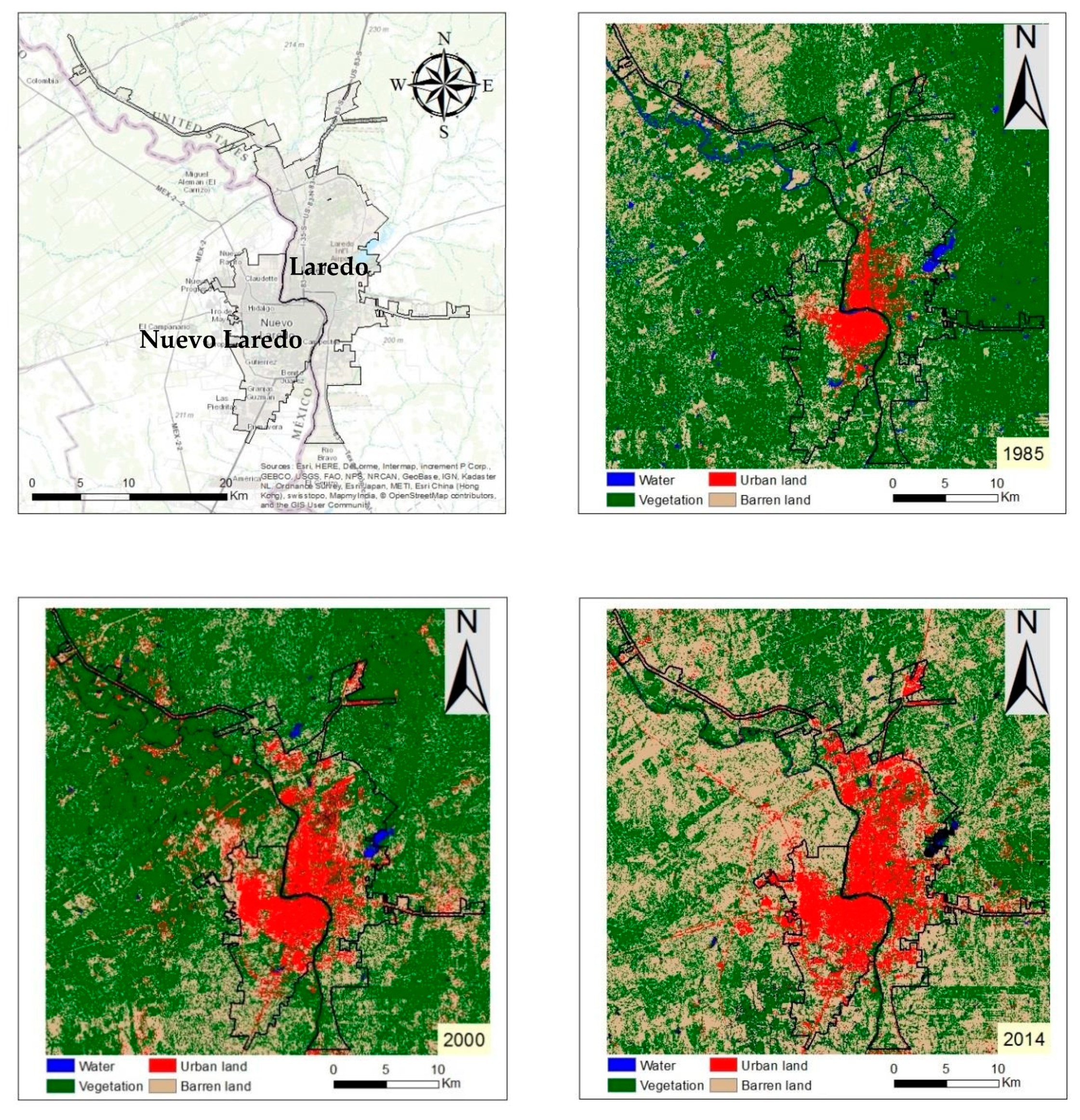
Laredo and Nuevo Laredo are bi-national metropolitan cities along the U.S.–Mexico border (Figure 1). The two cities are separated by the Rio Grande (i.e., Rio Bravo) River but are connected by four international bridges.

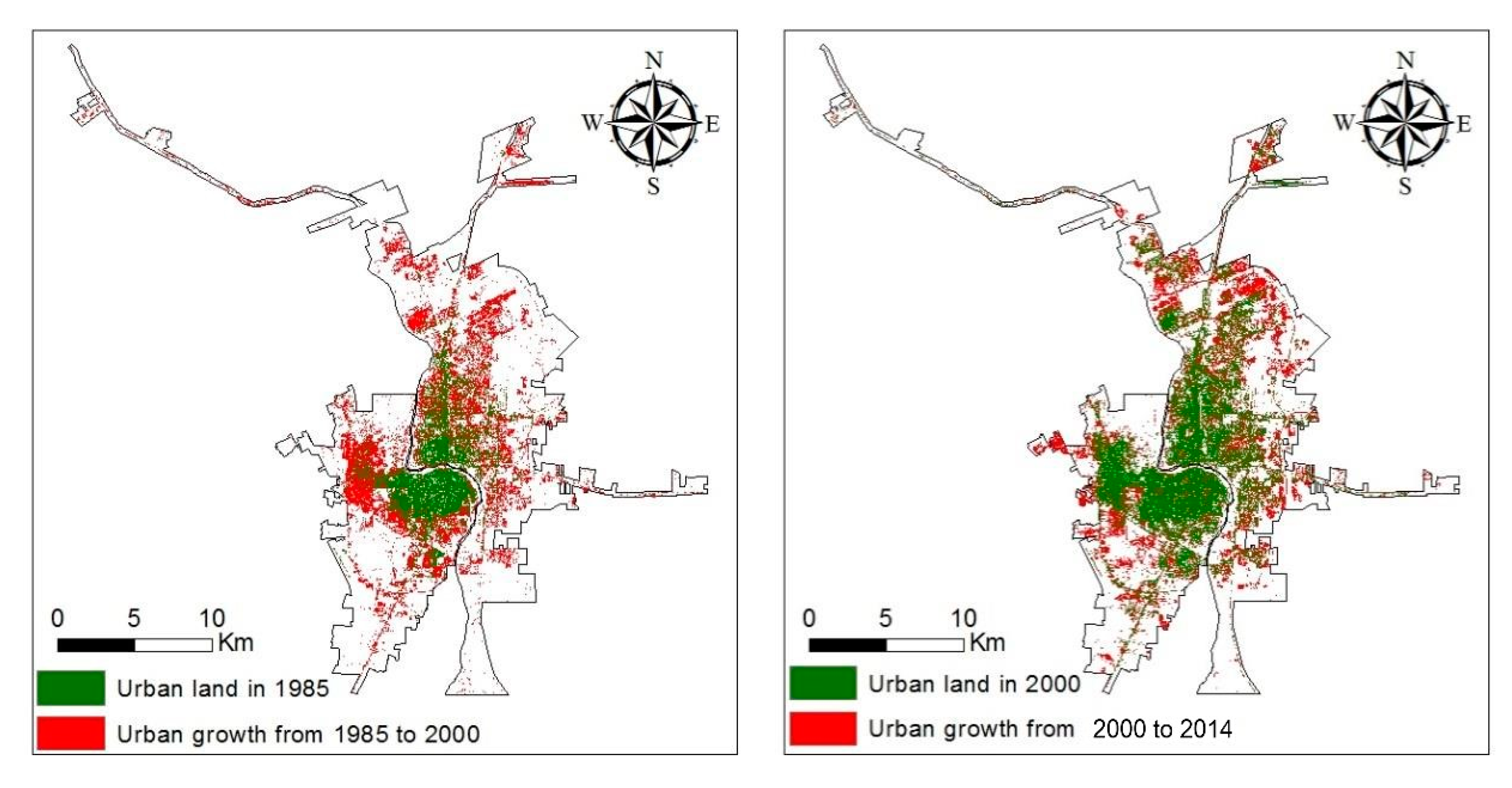
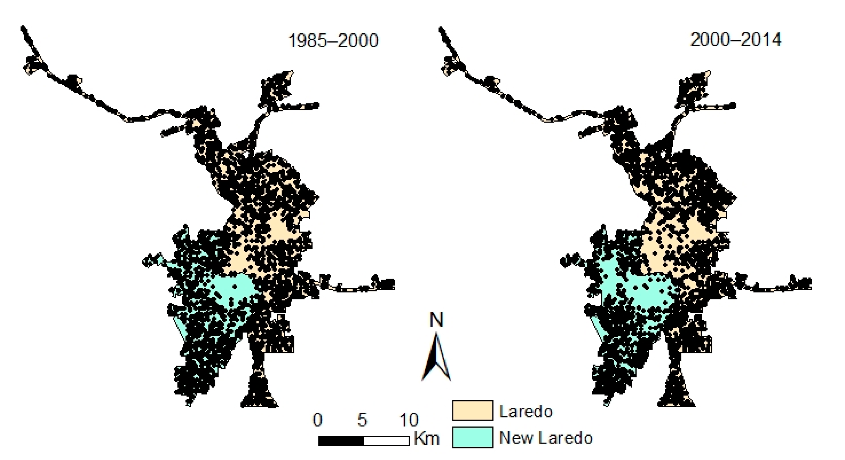
Landsat 5 Thematic Mapper (TM) imagery acquired in 1985 and 2000 and Landsat 8 Operational Land Imager (OLI) imagery acquired in 2014 from the United States Geological Survey (USGS) were downloaded for classification. Using a supervised maximum likelihood classifier in ERDAS Imagine, four categories of land cover were designated: built-up, vegetation, water, and barren land. Post-classification accuracy assessments resulted in a minimum 85 percent classification accuracy for each of the three dates. We then extracted only the built-up (urban) pixels which remained stable between classification dates and pixels that changed from non-urban land to urban land between 1985–2000 and 2000–2014, respectively, to perform the logistic regression analysis (Figure 2).

Based on expert knowledge from widely used urban growth models and some preliminary research on the U.S.–Mexico border, we made a selection of explanatory variables [19,20,21] for use in two models that correspond to two time periods (1985–2000 and 2000–2014). Common factors related to environmental and socioeconomic development were selected and generated to build the candidate explanatory variables. Considering the variable types and their relationship with the dependent variable, the explanatory variables were categorized into three groups: site specific variables, proximity variables, and density variables.

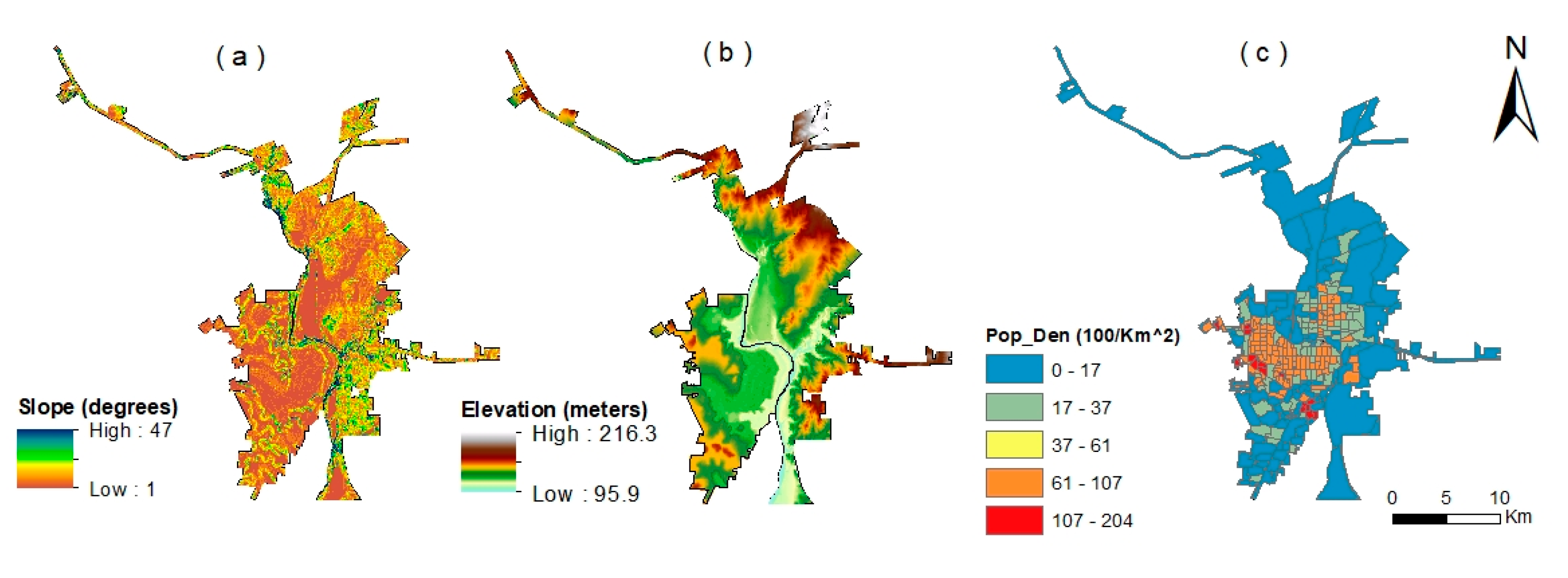
The first type of independent variable comprises site specific variables. Geophysical and topographic conditions affect urban growth in terms of accessibility and the cost of development and have been widely identified as strong factors for urban expansion [7,16]. For our study areas, positive effects of elevation and negative effects of slope have been documented [22]. We extracted the elevation and slope values for each pixel based on a corresponding 30 m digital elevation model (DEM) obtained from the USGS. We treated the geophysical and topographic conditions as constant variables for our study period. Population density is one of the most important demographic indicators of urban development [19], especially considering that a higher population density usually has greater labor and market availability and accessibility [22,23]. Taking data accessibility and comparability into consideration, the population density data at census track level for the years 2000 and 2005 were collected from the U.S.–Mexico Border Environmental Health Initiative (BEHI) website (Figure 3).

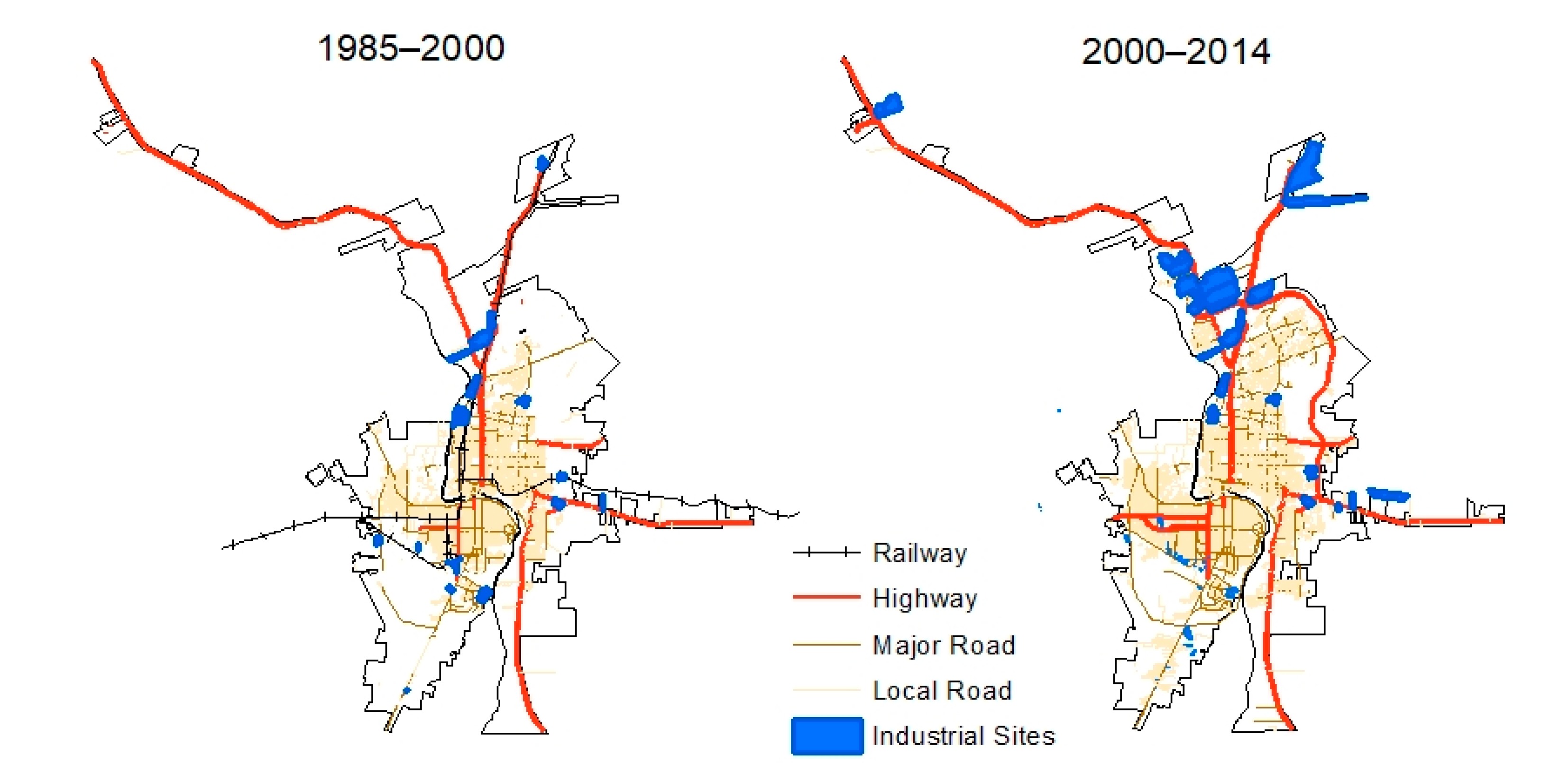
The second type of independent variable comprises proximity variables, which have been widely used in urban simulation models to explain land cover transitions [14,24,25]. Here, our proximity variables include distances to various types of transportation networks (highway, major roads, railroads), distance to industrial sites, and distance to existing urban clusters. Transportation data were obtained from the BEHI website for Laredo (2004) and Nuevo Laredo (2006). To ensure data reliability, we checked the BEHI data with transportation data available from the Texas Natural Resource Information System (TNRIS), the El Instituto Nacional de Geografía, Estadística e Historia (INEGI), and from the Instituto Municipal de Investigaciony Planeacion (IMIP). We manually edited roads by visual interpretation from Google Earth to create road networks for the years 1985 and 2000, separately. Considering the barrier of the Rio Grande River and the international border, Euclidean distances to the Rio Grande River and international bridges were calculated for each corresponding city. However, the distribution of local roads was highly spatially correlated with that of urban clusters (Figure 4). Thus, we did not include the factors related to the local roads (i.e., distance and density of the local road networks).

The international manufacturing plants (i.e., maquiladoras) program plays a considerable role in rates and patterns of urbanization in this border region [19]. Some studies have demonstrated that manufacturing-related industrial development along the U.S.–Mexico border has been an important factor of urbanization in this region [19,21]. We obtained industrial land boundaries from the Laredo city government website and INEGI (www.inegi.gob.mx) for the time period between 2000 and 2010. Then, we manually edited them by visual interpretation of Google Earth and satellite imagery to obtain industrial land boundaries for 1985 and 2000, respectively.

The third type of independent variable comprises density variables. Density conditions are often used in urban simulation models to explain land use transitions [25]. Theoretically, the transition from non-urban land to urban land is closely related to neighborhood conditions [11,15,25]. We selected several density attributes in 1985 and 2000, including existing urban clusters, transportation network, and industrial sites. In addition, we considered density variation due to scale. Four scales were used to generate density variables: 150, 300, 600, and 1200 m. However, high multicollinearities (>0.5) among different scales were detected for the respective density factors. Existing literature and urban simulation models have widely indicated that the possibility of urban growth at one site is distinctly attributed to local neighborhood conditions [9,10,11]. Moreover, considering that a 5 × 5 focal window size (i.e., 150 m) is commonly applied in CA models and as an attribute setting for neighborhood conditions [9,10], we used guidance from existing literature to generate density variables of 150 m for our analysis.

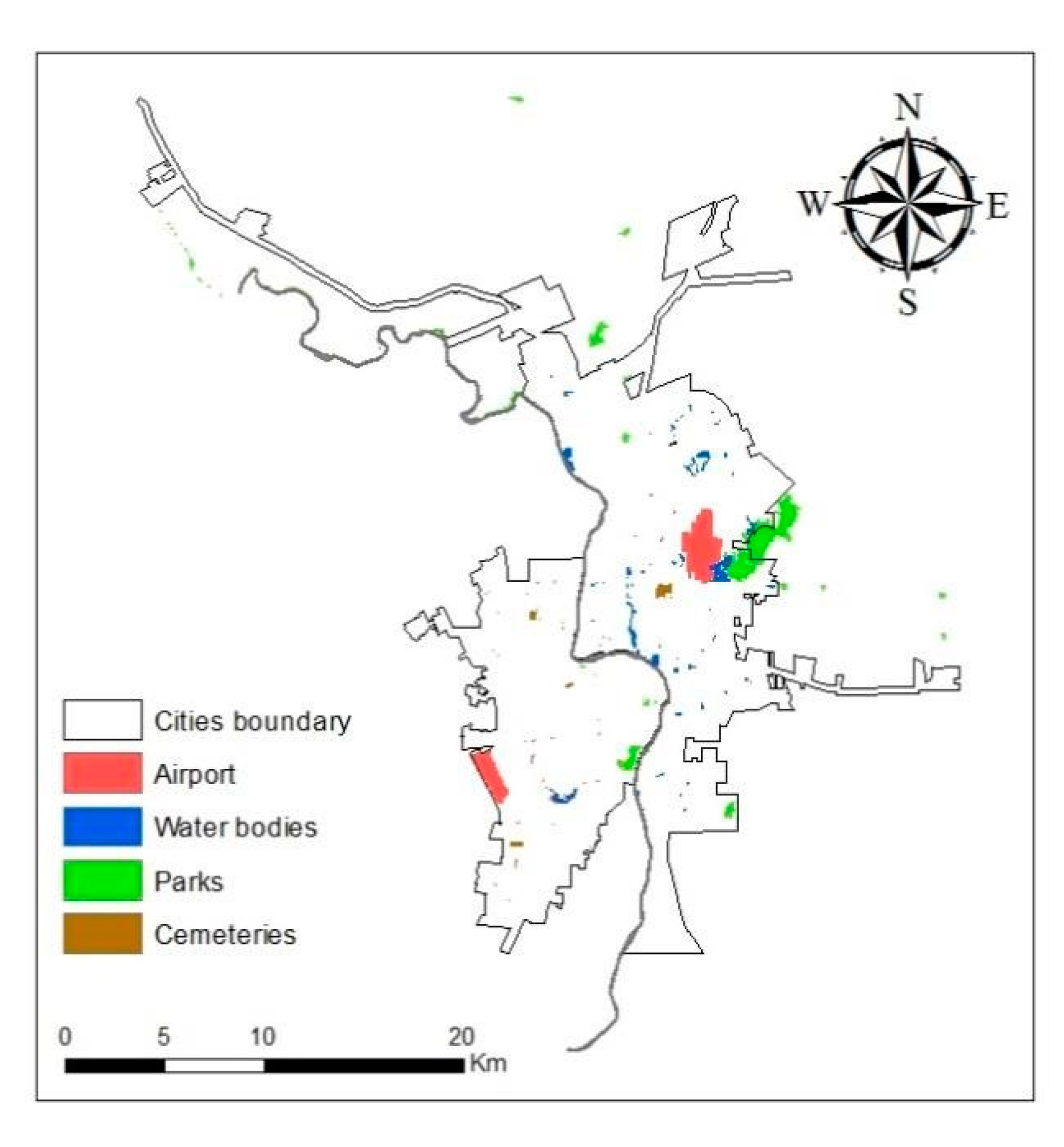
Finally, some areas were excluded from analysis given their low likelihood of urban land conversion. These areas included city parks, airports, water bodies, and cemeteries. These excluded areas for Laredo were collected from the City of Laredo government website. For Nuevo Laredo, the excluded areas were obtained from INEGI and digitized from the Landsat imagery (Figure 5).

3. Methods

3.1. Data Sampling and Multicollinearity Detection

Our study area consisted of 1412 × 1417 pixels at 30 m spatial resolution. We treated each cell, which incorporated potential attributes, as a potential sample for our regression analysis. Commonly, the presence of autocorrelation and multicollinearity are two issues in regression analysis. To mitigate spatial dependence and spatial autocorrelation, and to ensure that the sampling dataset represents the study area with enough information to understand urban growth patterns, a systematic random sampling scheme was designed to obtain the sampling points for the regression models for each time period. First, a regular grid of points spaced 210 m apart was created for the study area. Then, we selected half of the candidate points using the random selection tool in ArcGIS. This scheme is in accordance with previous research [14].

Finally, we used our final selected points to extract the cell values for both dependent and independent variables on which both the global logistic regression and logistic GWR were fitted. There were 836 and 782 samples for Laredo and Nuevo Laredo for the time period 1985–2000 and 1720 and 1704 for Laredo and Nuevo Laredo during the 2000–2014 time period (Figure 6). Thirteen candidate variables were extracted to the corresponding sampling points. A statistical summary of the variables associated with the sampling points for each study period is provided in

Table 1. Descriptive statistics of original collected dataset in this study.

	Description	Units	Date	Nuevo Laredo				Laredo
				Mean	Standard Deviation	Minimum	Maximum	Mean	Standard Deviation	Minimum	Maximum
Site specific variables
Elevation	Elevation of one specific pixel of 30 m*30 m	Meter	1985–2000	136.07	15.46	0.00	161.00	145.00	23.23	0.00	214.10
			2000–2014	136.42	15.73	0.00	161.00	146.34	23.05	0.00	214.10
Slope	The tangent of angle of surface to horizontal level	Degree	1985–2000	2.14	1.79	0.00	21.00	3.28	2.85	0.00	27.00
			2000–2014	2.12	1.66	0.00	15.00	3.36	2.90	0.00	35.00
Population_Den	Population density	100 per km2	1985–2000	44.23	2.84	0.00	203.94	6.45	10.33	0.00	47.28
X	The x coordinate of the sampling points	Meter	1985–2000	446.13	2.16	439.83	452.64	451.37	6.26	426.18	467.13
			2000–2015	445.90	2.19	439.83	452.64	451.67	0.15	426.18	467.13
Y	The y coordinate of the sampling points	Meter	1985–2000	3037.30	5.17	3027.63	3047.16	3047.85	9.60	3027.21	3069.00
			2000–2014	3037.08	5.29	3027.63	3047.16	3047.89	0.23	3027.21	3069.00
Proximity variables
Dis_Airports	Euclidean distance to airports for corresponding city	Meter	1985–2000	4586.30	2483.27	0.00	10,375.80	8360.25	6545.40	30.00	34,463.10
			2000–2014	4494.75	2568.53	0.00	10,375.80	8344.00	6837.42	30.00	34,463.10
Dis_RailWay	Euclidean distance Rio Grande River	Meter	1985–2000	3629.59	2505.45	0.00	10,276.20	4677.72	5469.29	0.00	28,156.50
			2000–2014	3827.82	2515.42	0.00	10,276.20	7569.95	124.65	123.69	28,308.40
Dis_River	Euclidean distance to railway for corresponding city	Meter	1985–2000	3862.33	1986.91	0.00	8136.20	3841.45	3153.67	0.00	14,466.00
			2000–2014	4078.45	1964.62	0.00	8136.20	58.53	0.00	0.00	10,001.50
Dis_Bridges	The Euclidean distance to the four international bridges	Meter	1985–2000	7477.92	3191.26	234.31	15,221.50	11,197.01	6401.62	189.74	36,039.00
			2000–2014	7830.80	3177.56	152.97	15,221.50	11,397.82	10,488.55	768.38	36,039.00
Dis_Industries	Euclidean distance to manufacturing plants for corresponding city	Meter	1985–2000	2606.09	1850.80	0.00	7804.67	4745.85	5330.43	0.00	28,422.70
			2000–2014	2700.33	1853.14	0.00	7804.67	2919.22	1738.06	0.00	14,704.90
Dis_HigMajWay	Euclidean distance to highway and major roads for corresponding city	Meter	1985–2000	846.15	651.70	0.00	4412.35	734.07	713.07	0.00	4804.59
			2000–2014	842.58	701.68	1.16	4105.09	499.56	331.34	0.00	3569.96
Dis_UrbanClust	Euclidean distance to urban clusters for corresponding city	Meter	1985–2000	429.63	484.97	0.00	3519.73	561.60	640.98	0.00	4639.05
			2000–2014	146.21	154.20	30.00	953.42	139.58	3.52	30.00	1073.31
Density variables
Den_HigMajWay	The number of pixels of highway and major roads within 5*5 neighbors	N/A	1985–2000	0.36	1.47	0.00	12.00	0.86	2.51	0.00	18.00
			2000–2014	0.43	1.60	0.00	12.00	0.75	0.06	0.00	22.00
De_Industries	The number of pixels of industrial pixels within 5*5 neighbors	N/A	1985–2000	0.24	2.01	0.00	25.00	0.35	2.59	0.00	25.00
			2000–2014	0.49	3.07	0.00	25.00	1.74	0.00	0.00	25.00
Den_UrbanClust150	The number of pixels of built-up land within 5*5 neighbors	N/A	1985–2000	1.06	3.17	0.00	22.00	1.02	2.98	0.00	25.00
			2000–2014	2.98	4.84	0.00	22.00	2.91	0.12	0.00	24.00

.

Prior to modeling, multicollinearity among the selected independent variables was tested in SPSS for the periods 1985–2000 and 2000–2014. Variables that exceeded the tolerance threshold for multicollinearity (0.5) were considered highly correlated. For example, existing urban clusters were closely related to the density of the local road network as well as population density. In addition, distance to the Rio Grande River was closely related to the elevation of the sampling points. In the case of multicollinearity, a single variable was selected for modeling. For both study periods, three covariates were excluded prior to conducting the regression: population density, distance to the four international bridges, and distance to urban clusters. Additionally, distance to the Rio Grande River and distance to the industrial sites were excluded for the period 1985–2000, while elevation, distance to railways, and distance to highways and major roads were excluded from analysis for the period 2000–2014.

3.2. Global Logistic Regression

Regression has been widely used to quantitatively analyze the driving forces of urbanization at different scales. The primary assumption of logistic regression for the analysis here is that the spatial pattern of land cover change is correlated with relevant explanatory variables that can be consistently measured on both sides of the U.S.–Mexico border [26]. In this sense, it enables us to incorporate different underlying factors of urban growth, including proximate effect, density effect, and road influence, into a spatially explicit model for specific sampling sites. In this way, logistic regression addresses ecological preservation and environmental protection practices.

The logistic regression statistical model supposes that the change probability of the land type of each grid can be represented in the form of a logistic function:

$$y={\beta }_0+{\beta }_1{x}_1+{\beta }_2{x}_2+\cdots +{\beta }_m{x}_m+e$$

(1)

$$y={\log }_e[P/(1-P)]=\log it(P)$$

(2)

$$P=\frac{e^y}{1+e^y}$$

(3)

Equation (1) is the regular regression, where $x_1, x_2,\dots ,x_m$, are the explanatory variables, y is the dependent variable, ${\beta }_1$,${\beta }_2$, …, ${\beta }_m$ are the regression parameters to be estimated, and e is the residual error. In this case, land change is treated as a Bernoulli variable (0: no change, 1 change to urban land). If we just use regular regression (1) to model the urban growth, the errors cannot be normally distributed, and the estimated value will be beyond the range of 0 to 1. Therefore, the linear combination function of the independent variables is represented by logit (P), as shown in Equation (2). P is the land transition probability from non-urban to urban. $\left(P|1-P\right)$ is the odds ratio of the land type change. Equation (2) can also be shown in the way of Equation (3), where the probability P will increase with value y, and at the same time, it ensures that the probability surface will be continuous within the range of 0 to 1.

We used the logistic regression model in SPSS and GWR 4.0 to perform the analyses. GWR 4.0 software, which was created by Fotheringham et al. [27], is free to use and open source. GWR 4.0 provides a range of options to select different kinds of regression. In addition, the outputs are easily incorporated into ArcGIS for visualization [28].

3.3. Logistic GWR

The logistic regression model developed in the preceding session is global, in the sense that the partial relationships between the independent variables and dependent variable are assumed to be stationary across the entire study area [29]. Logistic GWR, on the other hand, can accommodate non-stationarity by incorporating geographic location into the models. Since every point in space is taken into account when fitting the regression equation, GWR is a powerful method to understand the spatial distribution of variables and explore the spatial heterogeneity of relationships and processes over the entire space [27].

Global logistic regression is typically single-valued, while the Logistic GWR is multi-valued: different locations have different statistical values in the space. Modified from the global logistic regression, the logistic GWR equation is as follows:

logit (P_i) = log_e (P_i|1 − P_i) = β₀ + β₁x_1i + β₂x_2i + … + β_mχ_mi + ε_i

(4)

where $x_{1i}, x_{2i},\dots ,x_{mi}$ are the independent variables at location i, and ${\epsilon }_i$ is the regression residual at location i. Instead of remaining the same everywhere, ${\beta }_1$,${\beta }_2$, …, ${\beta }_m$ vary in relation to location i.

Essentially, a logistic regression is created for each instance in a spatial dataset based on a selection of surrounding instances. A distance band, or kernel, must be specified to determine how much influence each occurrence exerts on the others. This kernel determines the number of surrounding data points that are included in the localized regression equation of the data point being regressed. An effective spatial sampling scheme can significantly account for the spatial dependence problem by expanding the distance between the sampling points. Furthermore, spatial autocorrelation effects can be largely reduced, since the interval distance between sampled sites is usually larger than that between the neighboring points in the original dataset [22].

4. Results and Discussion

4.1. Logistic Regression Analysis

Overall, the global logistic regression model resulted in moderate goodness of fit, with −2 Log likelihood values of 2433.01 and 2369.87 for the time periods 1985–2000 and 2000–2014, respectively (

Table 2. Global logistic regression results for the probability of conversion from non-urban to urban.

Independent Variables	1985–2000			2000–2014
	β	S.E.	Odds Ratio	β	S.E.	Odds Ratio
Site specific variables
Elevation	0.001	0.003	1.001	---	---	---
Slope	−0.101	0.026	0.904	−0.041 (*)	0.024	0.96
Proximity variables
Dis_Airports	0.000 (***)	0.000	1.000	−0.092 (***)	0.014	0.913
Dis_RailWay	0.000 (***)	0.000	1.000	---	---	---
Dis_River	---	---	---	0.000	0.000	1.000
Dis_Industries	---	---	---	−0.067 (*)	0.029	0.936
Dis_HigMajWay	−0.001 (***)	0.000	0.999	---	---	---
Density variables
Den_HigMajWay	0.090	0.024	1.094	0.075 (***)	0.019	1.078
Den_Industries	0.030 (***)	0.019	1.031	0.046 (***)	0.01	1.047
Den_UrbanClust150	0.172 (**)	0.021	1.187	0.132 (***)	0.011	1.142
Sample size	2556			2486
−2 Log likelihood	2433.055			2369.868
Cox and Snell	0.197			0.162
Nagelkerke	0.286			0.239
PCP	77.5			78

Note: β: coefficients in Equations (1) and (4). S.E.: standard error. Please refer to the full variable names from Table 1. ^(*): significance at 0.05 level; ^(**): significance at 0.01 level; ^(***): significance at 0.001 level. PCP: the percentage correctly predicted with cut value 0.5. ---: the variable was not included in regression analysis due to multicollinearity.

). The overall percentages of cases correctly classified were 77.5 and 78.0 at 1985–2000 and 2000–2014, respectively. These percentages indicate that both models were relatively successful at predicting whether or not an observation (pixel) in our dataset did or did not convert to urban land cover in a given time period. However, for parameter β, which indicates the contribution of each variable to the probability of urban conversion, the odds ratio is more intuitive to explore factors that contributed to land cover change. Using slope during 2000–2014 as an example, the value of the odds ratio 0.96 means that the slope increase of one degree at one specific pixel would have a decreased probability (96%) to change to built-up land. However, Norman et al. [19] found that steep slopes did not appear to be a limiting factor for Nogales, Sonora (Mexico), which is different from the situation in Nogales, Arizona (U.S.), where buildings are designed and planned to only be situated on desirable topographic sites.

For the time period 1985–2000, of the eight input variables for the regression analysis, distance to airports, distance to the rail way, distance to highway and major roads, density of industrial sites, and density of existing urban clusters within 150 meters were all significantly related to urban growth. Among them, two density variables (density of industrial sites and density of existing urban clusters within 150 m) were highly related to urban growth, with odds ratios of 1.031 and 1.187, respectively. Since both of their odds ratios were greater than 1, we can infer that the probability of urban development in areas with higher industrial site density or existing urban clusters was much higher than the probability of urban growth in areas with lower densities. For proximity effects, the odds ratio of distance to highways and major roads was 0.999, which means that the urban growth probability of pixels 1 km further away from highways or major roads was 0.999 times as large as the growth probability of that area.

For the analysis period 2000–2014, there were seven variables incorporated into the regression analysis: slope, distance to airports, distance to industrial sites, distance to the Rio Grande River, density of existing urban clusters, density of industrial sites, and density of highways and major roads (Table 2). Except for distance to the Rio Grande River, all explanatory variables were significant. Most of them were significant at α ≤ 0.001, except the slope, which was significant at α ≤ 0.05. In terms of the factors for contributing to urban growth between 2000–2014, elevation, distance to the Rio Grande River, and distance to the railway did not affect urban land cover change within the study area. Regarding the effect of the river, this finding is similar to the results from a study which illustrated that distance to the Yangtze River was not a factor influencing the probability of urban growth in Wuhan (Hubei province, China) [25].

It is worth noting that the three density variables (density of industrial sites, density of existing urban clusters, and density of highways and major roads) all had a positive effect on urban growth, with a very high level of significance between 2000–2014. Notably, a high level of density of urban clusters was estimated as 1.142 times as large as the probability of urban development compared to an area with lower urban density. It also implies that urban growth was highly dependent on the highway and major roads infrastructure of both cities between 2000 and 2014. In terms of the proximity effects between 2000 and 2014, the greater distances to airports and to industrial sites, the lower the likelihood of urban land cover conversion.

The positive effect of nearby urban clusters is in accordance with prior findings [14,22,25] and confirmed by results from some of the urban growth models based on CA theory [9,11,15,16]. Similarly, the effect of industrial site density was also significant for urban growth in both cities. With an odds ratio greater than one, it indicates that a higher probability of urban change occurred for pixels with a higher density of industrial sites. For both cities, the influences of the highway and major roads infrastructure on urban growth were indicated by their proximity effect between 1985 and 2000 and their neighborhood effect between 2000 and 2014, respectively. This is not surprising as this situation is in agreement with prior research findings [7,14,16,30].

4.2. Diagnostics of Logistic GWR

While the global logistic regression model provided an explanation of the underlying factors of urban growth in the two cities, the spatial variation of the underlying factors was not characterized. Global regression methods can only represent the general trend of the study area and may ignore considerable local variations [27]. In this case, logistic GWR is an effective method to detect spatial variation of the estimated factors. Here, we used the same sample points to build the logistic GWR model. The −2 Log likelihood and the PCP indicate that the GWR had better goodness of fit and improved performance (

Table 3. Diagnostic information of logistic geographically weighted regression (GWR) during 2000–2014.

Logistic GWR Result
	β	Lower Quartile β	Median β	Upper Quartile β
Slope	−0.041	−0.051	−0.035	−0.027
Dis_Airports	−0.092	−0.135	−0.079	−0.037
Dis_River	0.000	0.000	0.000	0.000
Dis_Industries	−0.067	−0.114	−0.095	−0.081
Den_UrbanClust150	0.132	0.109	0.131	0.148
Den_Industries	0.046	0.012	0.028	0.045
Den_HigMajWay	0.075	0.052	0.060	0.066
Constant	−0.883	−1.020	−0.800	−0.552
Comparison of logistic GWR and global logistic regression
	Global logistic regression	Logistic GWR
−2 Log likelihood	2369.868	2265.202
Global AIC	2385.868	2307.967
PCP	78.0	78.6

Note: β coefficients and intercept in Equation (4). AIC refers to Akaike information criterion. Please refer to the full variable names from Table 1.

).

The global logistic regression model has unified parameters across the entire study area. However, the GWR exhibited considerable variation in terms of the β parameter, although there was no variation from positive to negative or from negative to positive (Table 3). The comparison suggests that global regression exhibits challenges associated with spatial stationarity, while GWR can mitigate this problem. The distance to and density of industrial sites had the highest difference of β between the global logistic regression and the logistic GWR. This suggests that industrial sites tend to have greater local influence on urban growth. At the same time, major city centers tend to affect urban growth globally. Moreover, we can see that the distance to airports had the largest spatial variation. Density of existing urban clusters also exhibited considerable spatial variation.

4.3. Results of Logistic GWR and Spatial Non-Stationarity Relationship

Unlike global logistic regression, the logistic GWR generated a set of estimated coefficients and the associated pseudo t-statistics for each sampling point. Using these values, we spatially interpolated a continuous surface using the inverse distance weighted (IDW) interpolation using the Spatial Analyst Toolbox in ArcGIS. Hence, the surfaces of the estimated coefficients and t-statistics were generated to reveal the spatial variations of the underlying factors behind the urban growth. Figure 7, Figure 8, Figure 9, Figure 10 and Figure 11 demonstrate apparent spatial variation across Laredo–Nuevo Laredo.

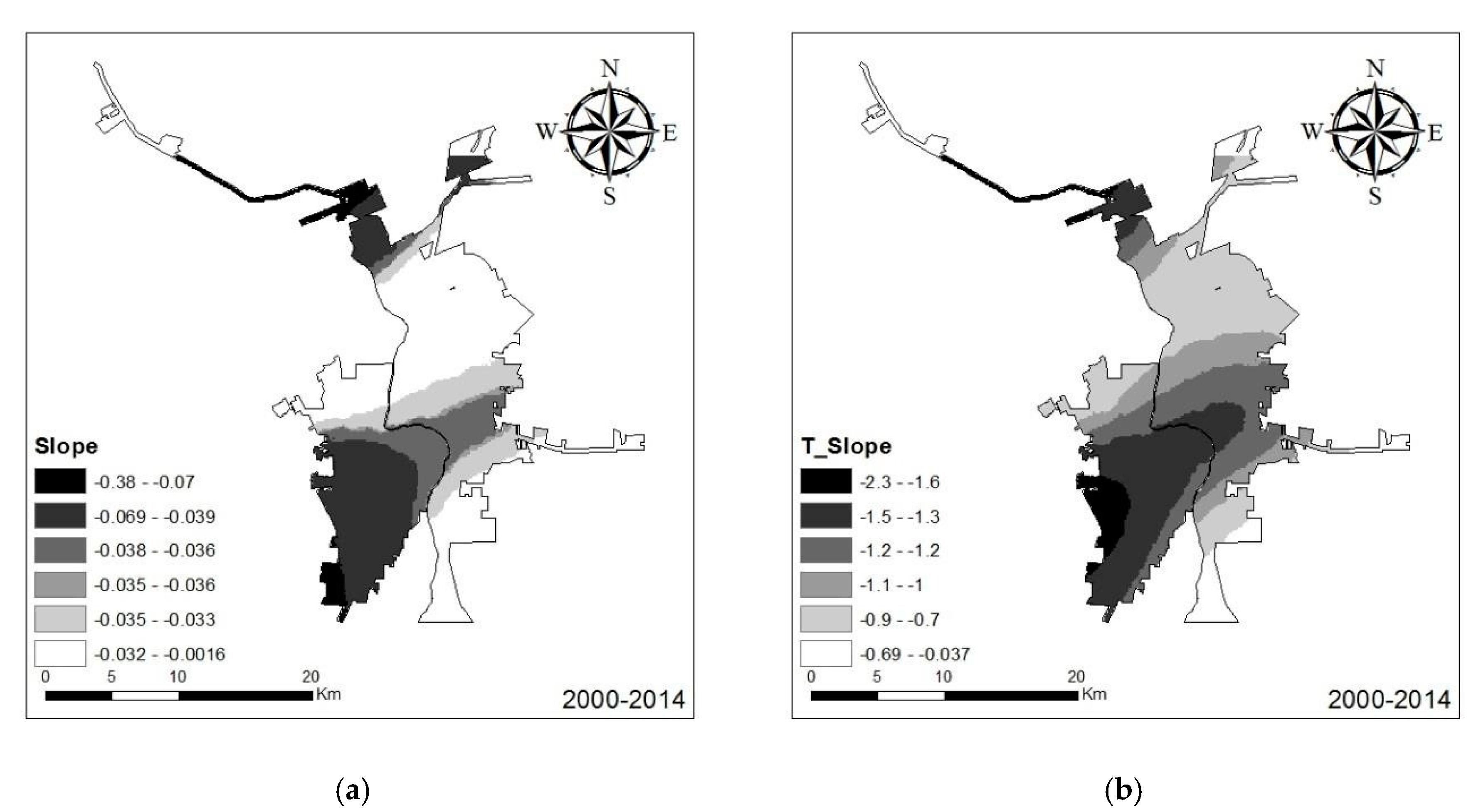
Based on Figure 6, slope did affect urban growth for most of the study area between 2000 and 2014, which is similar to the result from the global regression. As Figure 7 demonstrates, the spatial distribution of the t-statistic of slope generally coincides with the spatial distributions of the slope coefficient, which together indicate that there was a considerable part of the study area where the slope parameter was not significant in explaining urban land cover change. For the remaining portion of the study area, slope had a more significant negative effect on urban growth in Nuevo Laredo than Laredo, especially in the southwest portion. For Laredo, only a small portion in the northern region showed slope having a significant effect, as exhibited by the estimated coefficient t-statistic (Figure 7). These results indicate that in the southwestern area of Nuevo Laredo, slope had a highly negative effect on urban land cover change and that new urban cells were more likely to occur in areas with low slopes.

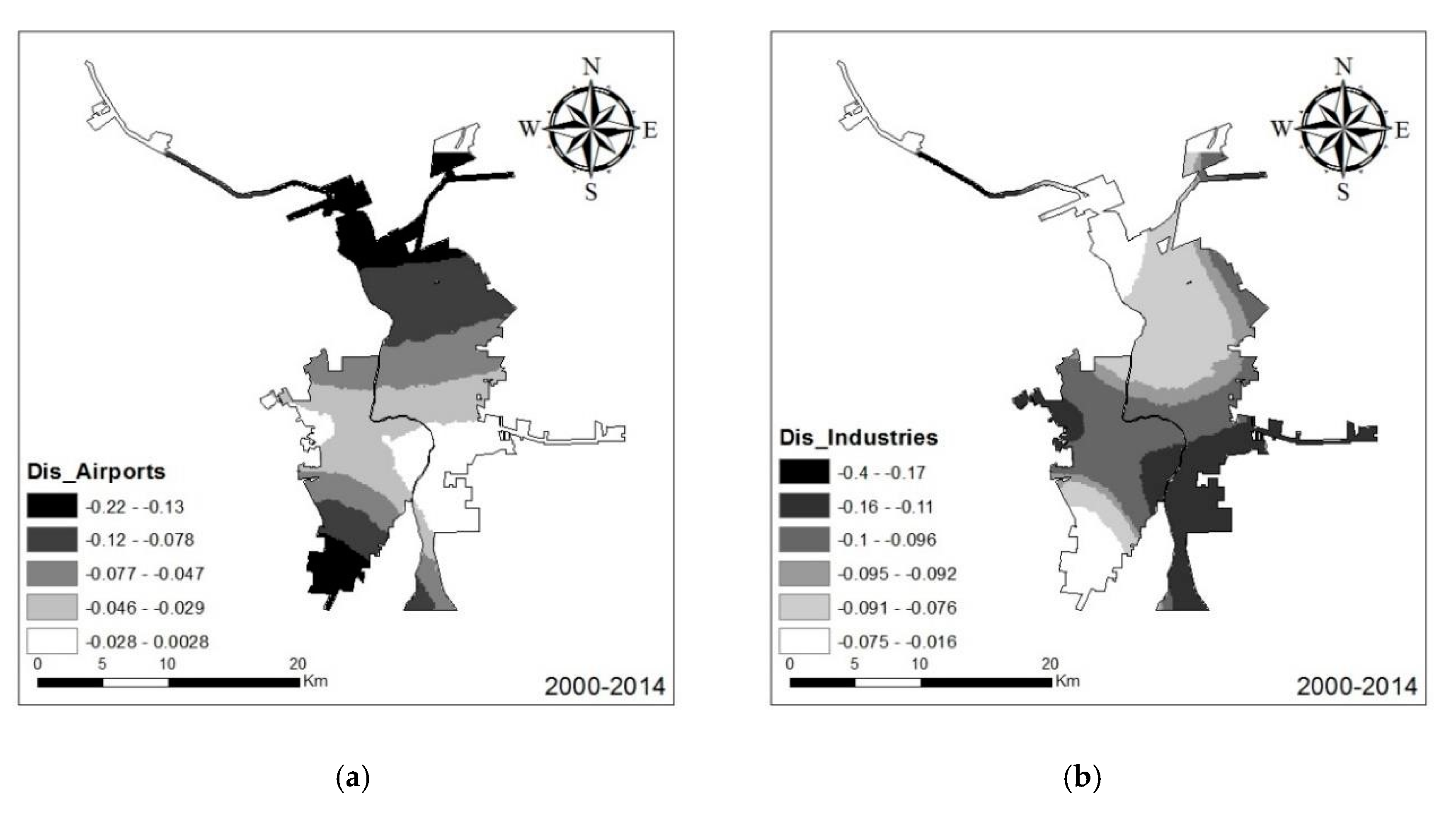
Figure 8 shows the spatial variation in the effect of two proximity variables: distance to airports and distance to industrial sites for the 2000–2014 analysis period. While the negative effects had been modeled by the global logistic regression model, proximity effects also varied throughout the study area. Distance to airports exerted greater negative influence on urban development in the southern portion of Nuevo Laredo and the northern portions of Laredo (Figure 8). In particular, this effect was insignificant in the area around the Nuevo Laredo airport. In contrast, the estimated parameter surface of the distance to industrial sites suggests that the pixels closer to industrial sites exhibited a higher probability of transitioning to urban land cover. Compared to the global logistic regression model results, the logistic GWR more clearly showed the role of proximity to industrial sites.

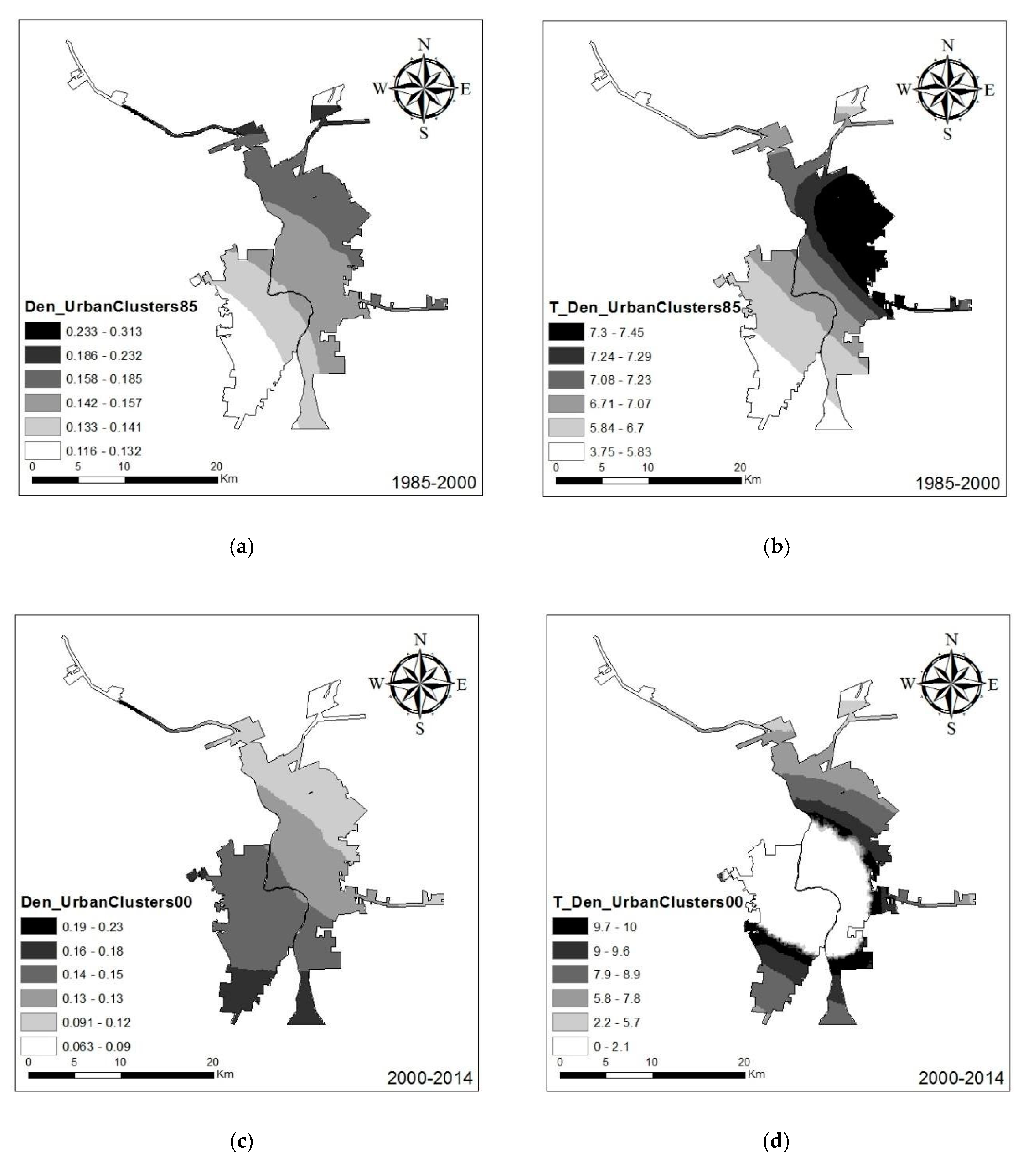
The density of existing urban clusters had a strong positive influence on urban development of both cities for both time periods, which is similar to the results from global regression (Figure 9). During 1985–2000, the effect of existing urban clusters for urban growth was much more apparent in Laredo than Nuevo Laredo. In contrast, between 2000 and 2014, these effects were much more apparent in Nuevo Laredo than Laredo. This is understandable because during 1985–2000, the new urban areas in Laredo were adjacent to existing urban clusters in 1985, with a much higher growth rate than Nuevo Laredo (11.72% annual growth rate for Laredo versus 6.97% annual growth for Nuevo Laredo). However, between 2000 and 2014, growth in Nuevo Laredo exhibited increased densification of existing urban clusters, while Laredo showed a more dispersed (i.e., sprawl) growth pattern. The t-statistic surface corresponds with the estimated coefficient during 1985–2000 (Figure 9). Interestingly, the central part of the study area did not show significant urban growth, as evidenced by very low t-statistic values, while the surrounding adjacent areas had very high t-statistic values. The reason for this strong contrast is that the central part of the study area had already experienced urban densification, while urban growth in the remaining area relied more on nearby urban clusters.

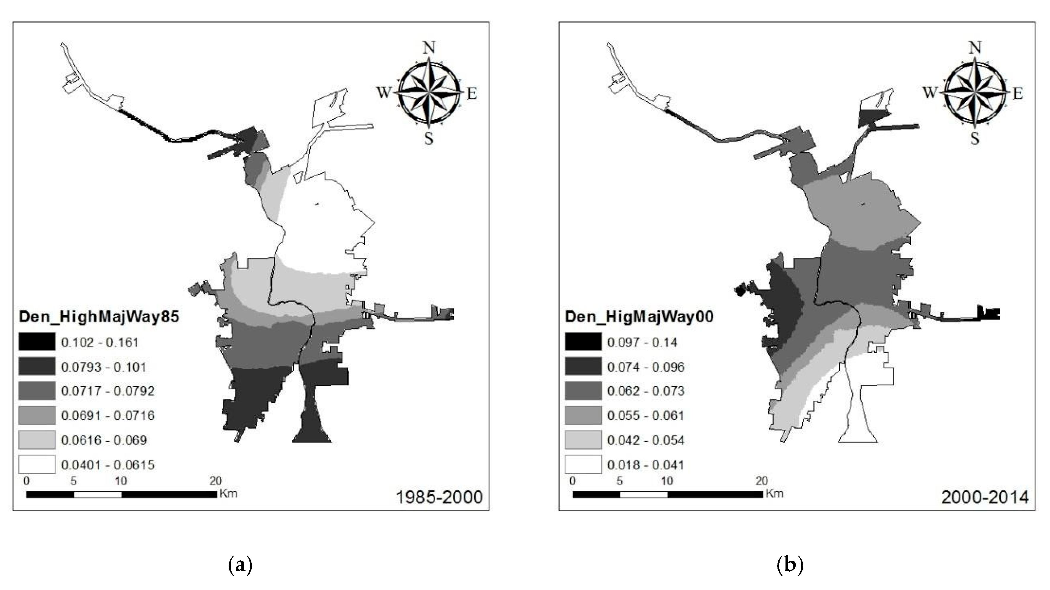
Between 1985 and 2000, the density of highways and major roads had a stronger positive effect on most parts of Nuevo Laredo than Laredo (Figure 10). This effect was most noticeable in the southern part of Nuevo Laredo, where there was an absence of a local transportation network. The density of the highway and major roads had a strong positive effect on the urban growth. On the contrary, in the far north and far south of Laredo, where the highway exists, the density of the highways and major roads variable showed a slightly positive effect on the urban growth compared to the remaining area.

Between 2000 and 2014, the effect of highways and major roads density was relatively lower, with the estimated coefficient ranging from 0.02 to 0.14 and considerable spatial variation in the parameter significance (Figure 10). The effect of highway density in this period was more prevalent for Laredo compared to the 1985–2000 time period, as evidenced by the estimated coefficient surface. This difference in driving mechanism was related to the economic and development backgrounds of the two countries. The effect of highways on urban development in developed countries such as the U.S. was also suggested by Reilly, O’Mara et. al. [30] in their studies based on logistic regression analysis.

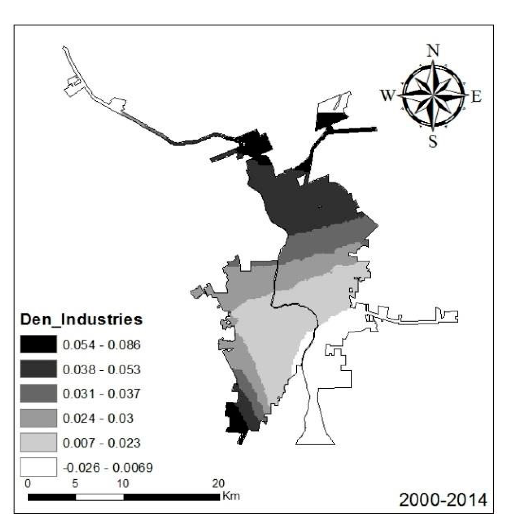
The last underlying factor that we used to study urban growth was the effect of industrial sites. It is noteworthy that the distance to industrial sites only influenced urban growth in the time period of 2000–2014, rather than 1985–2000 (Table 2). Industrial site density exhibited spatial variation in the form of a positive effect in the southern and southwestern regions of Nuevo Laredo and in Northern Laredo. Industrial site density had a slightly negative effect on urban growth in Southeastern Laredo (Figure 11). This distribution is associated with the spatial position of the industrial sites of both cities.

4.4. Methodological Implications

Regression is one of the most popular approaches used to understand the driving forces behind land cover changes. While the global logistic regression model allows us to characterize the factors that influence urban growth, the logistic GWR more efficiently and accurately assesses the underlying factors that drive urban growth based on spatial variation.

Our findings related to the influencing factors of urban growth are similar to results from some other models based on CA theory [31,32]. However, this study area exhibits unique characteristics. As the largest land-based port between the U.S. and Mexico, the study area plays a unique and indispensable role in connecting the two countries. Nonetheless, to detect the mechanism and trajectories of the urban growth, an analysis at a much larger, regional scale is necessary.

Previous studies have focused on analyzing urban growth for single cities, while research on broad areas is far less common. Due to its unique manufacturing characteristics, urban land growth in this area was much faster than that of megacities in the U.S. during the same period and is comparable with the average growth rate of the fast growing county-level cities in China during the same period [33]. Several surrogate variables, such as industrial development patterns and construction of transportation infrastructure, were easily quantified on both sides of the border. Moreover, we did find spatial variations in the relationships between these factors and urban growth.

The comparison of the analysis results shows that, for our study area, the logistic GWR outperformed global logistic regression with respect to goodness of fit and that logistic GWR can illustrate the spatial variation of estimated factors, thus providing a better understanding of the spatial patterns of urban land cover change. There is some literature that explains and justifies the choice of GWR to explore local spatial patterns [34], whereas our study indicates that the choice of global or local regression in geographic analysis depends on the context of the question being asked. For our study area, which includes an international boundary, logistic GWR can be used as a complementary model to explore the urban growth effect and whether the international border strongly influences urban growth. Our results indicated that the international border has a significant effect.

Nevertheless, there are still several limitations of this study on this border area regarding logistic GWR and global logistic regression. For example, Mexico’s manufacturing plants program is a symbol of economic globalization which is likely influenced by distant or indirect drivers of urban growth [19]. It is believed that the external patterns and processes of trade, migration, and policies affect urban growth on both sides of the U.S.–Mexico border. However, these factors are not directly quantified and incorporated in empirical studies. Therefore, future research to characterize these types of indirect drivers of urban growth and incorporate unobservable institutional factors across national borders is warranted. The study was based on statistical analysis in the time periods of 1985–2000 and 2000–2014. During the study periods, spatial regulations may have changed, which could lead to uncertainty as to the interoperation of results. In addition, data accessibility with consistent socioeconomic datasets at equal time intervals prevented a comprehensive analysis of the trajectories of urban growth throughout the historical range.

5. Conclusions

In this study, we used global logistic regression and logistic GWR to investigate factors influencing urban growth in Laredo, Texas, U.S. and Nuevo Laredo, Tamaulipas, Mexico from 1985 to 2014. For the time period 1985–2000 of analysis, the global logistic regression and the logistic GWR show that two density variables, density of existing urban clusters and density of industrial sites, influenced urban development, with observable spatial variation. Additionally, the underlying factors changed with time and became more complicated. Between 2000 and 2014, there were two proximity variables (distance to airports and distance to industrial sites) that influenced urban land cover change and three density variables (density of existing urban clusters, density of industrial sites, and density of highways and major roads) that influenced urban growth. In summary, our results indicate that the logistic GWR is in overall agreement with the global regression, with the same influencing direction for all estimated factors except density of industrial sites between 2000 and 2014. The performance of the models suggests that the local models are complementary to global models to empirically analyze the determinants of urban growth in study areas that contain a political border. Overall, this study contributes to an improved understanding of drivers and patterns of urbanization along the U.S.–Mexico border region. Specifically, the border brings different socioeconomic conditions (e.g., population, industrial sites) of two cities, which affects the overall urban growth rate and extent, as evidenced by both the global regression and GWR model results. In addition, the GWR analysis further contributes to explaining the spatial heterogeneity characteristics of urban growth across an international border. Information related to the spatial variability of relationships between urban growth and neighborhood and proximity effects provides insight into the complexity and interconnections between land use change and associated factors.