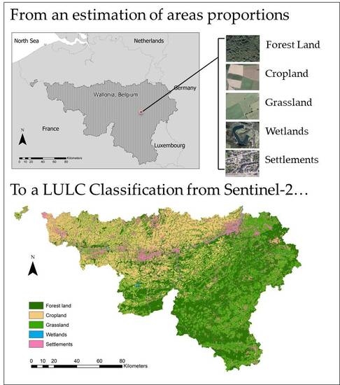
Use of Sentinel-2 and LUCAS Database for the Inventory of Land Use, Land Use Change, and Forestry in Wallonia, Belgium


Abstract
1. Introduction
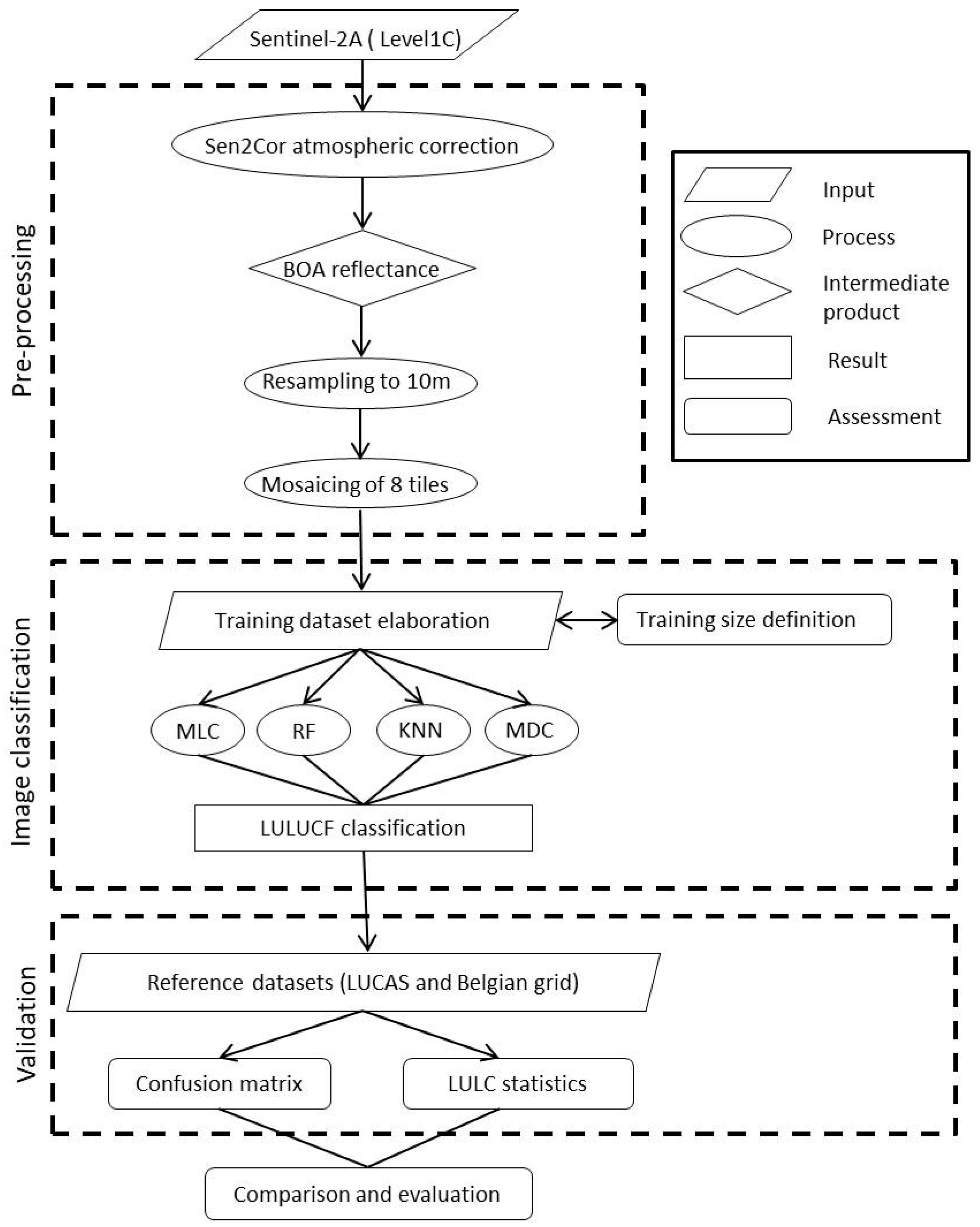
2. Materials and Methods
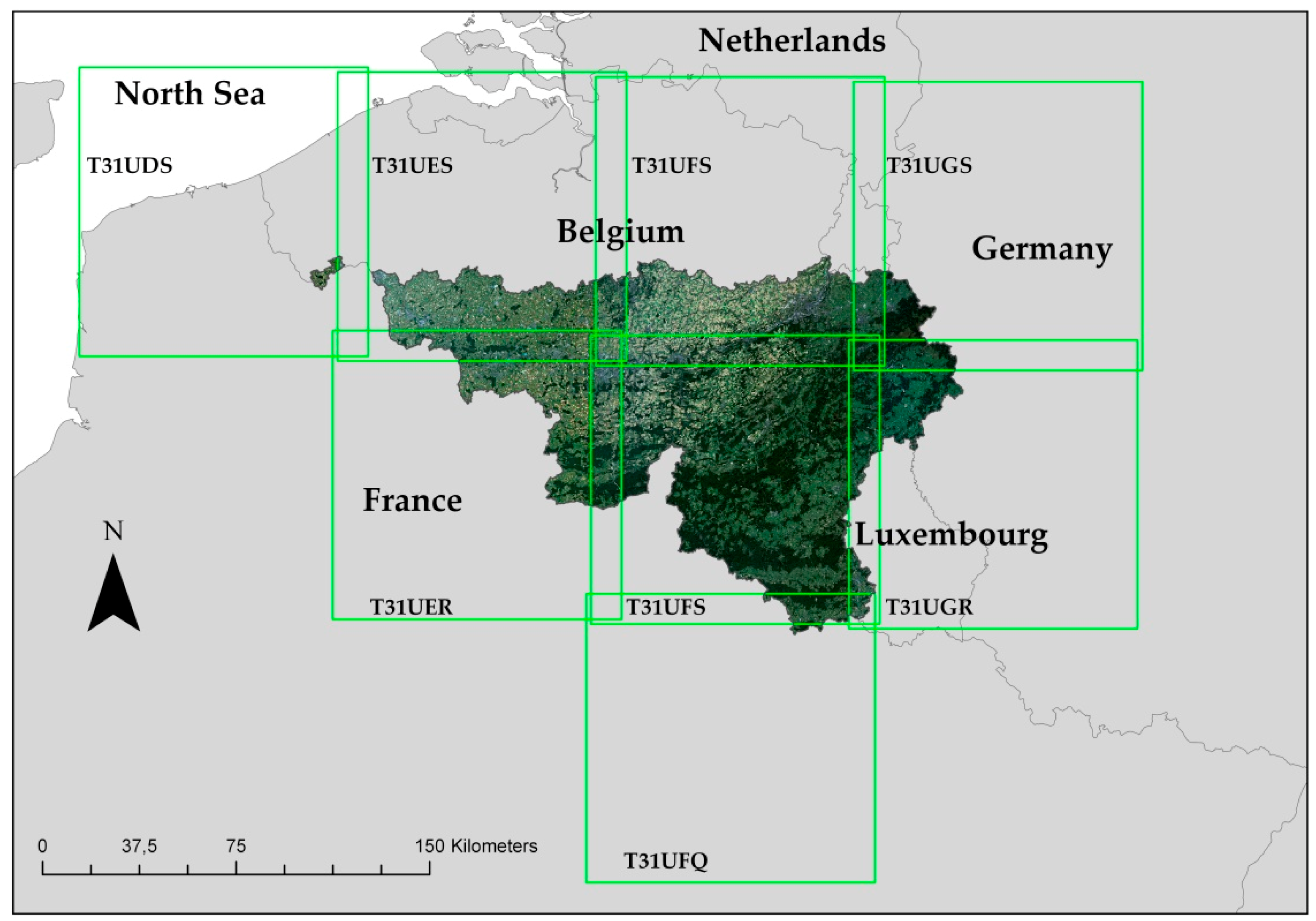
2.1. Sentinel-2 Data
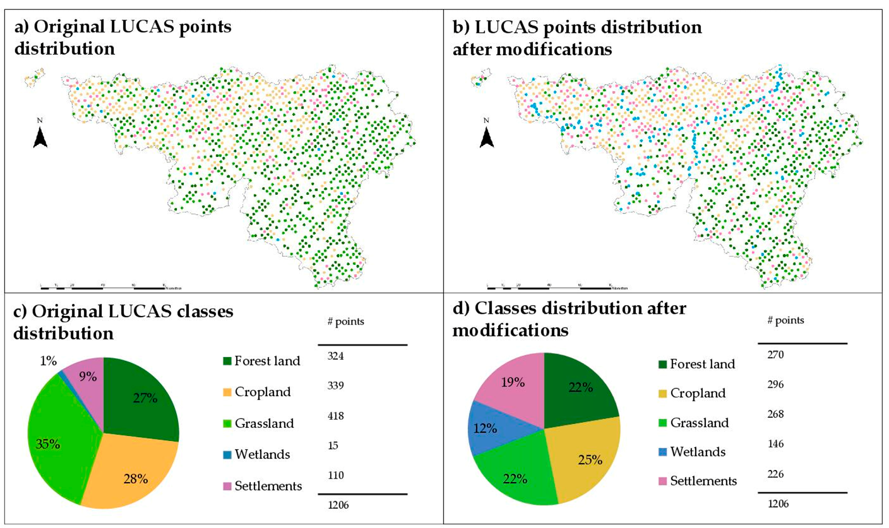
2.2. LUCAS Dataset
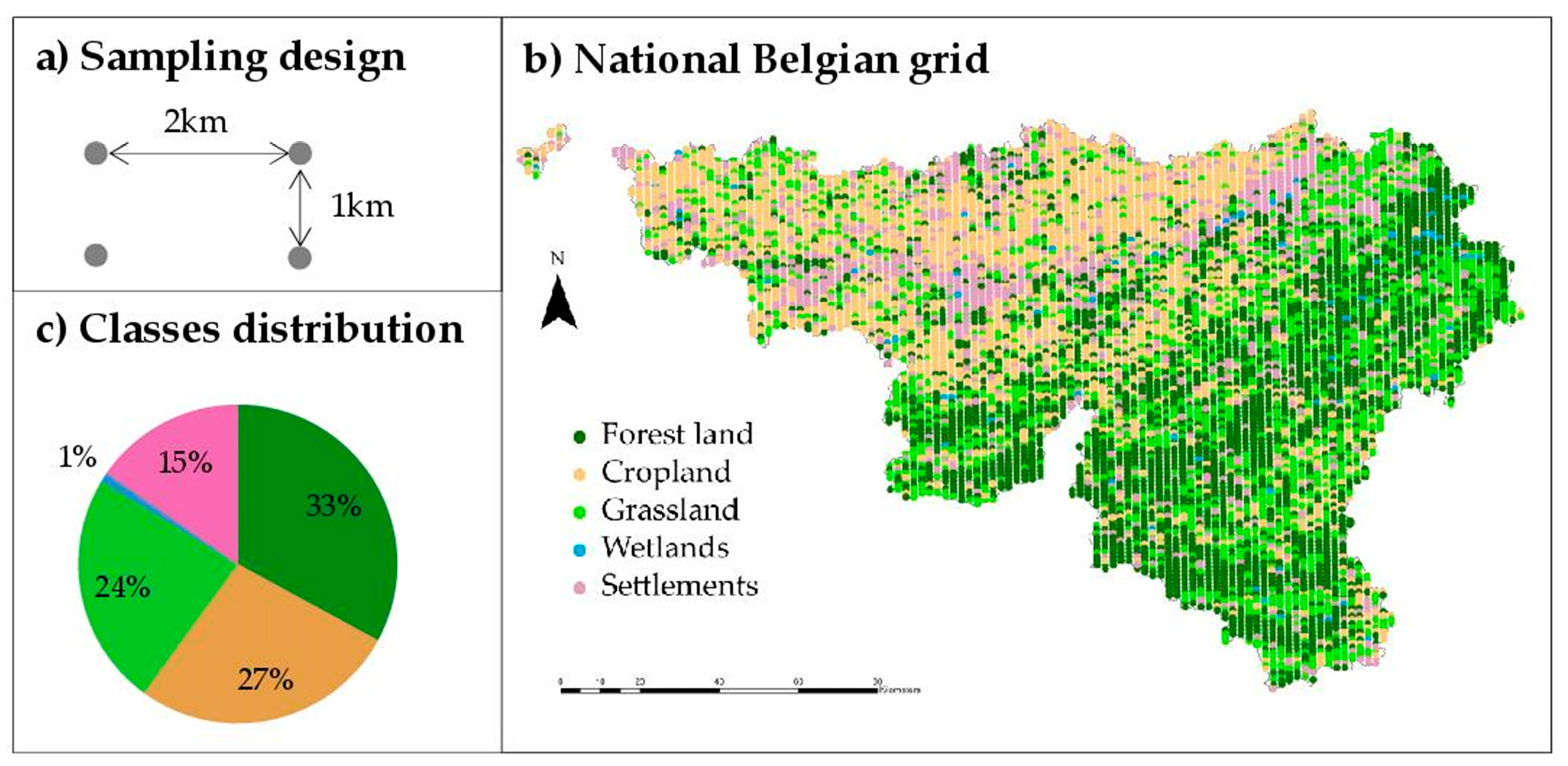
2.3. National Belgian Grid Dataset
3. Results
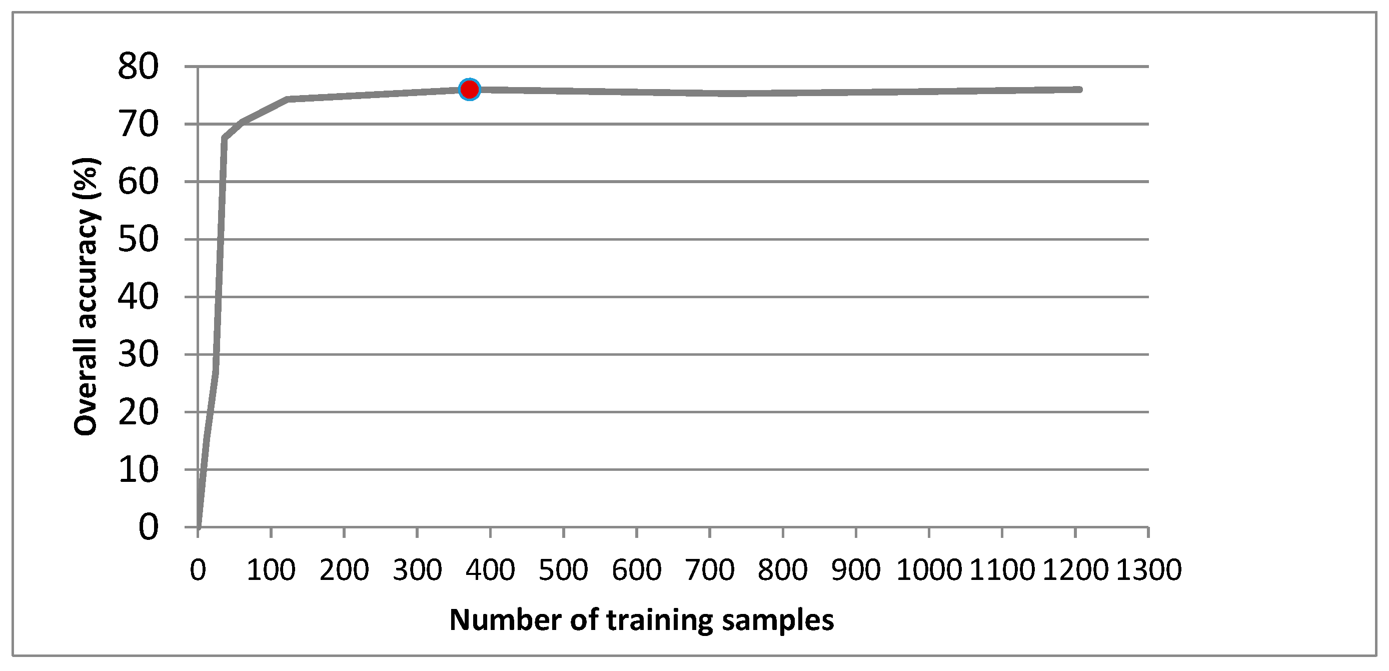
3.1. Training Size
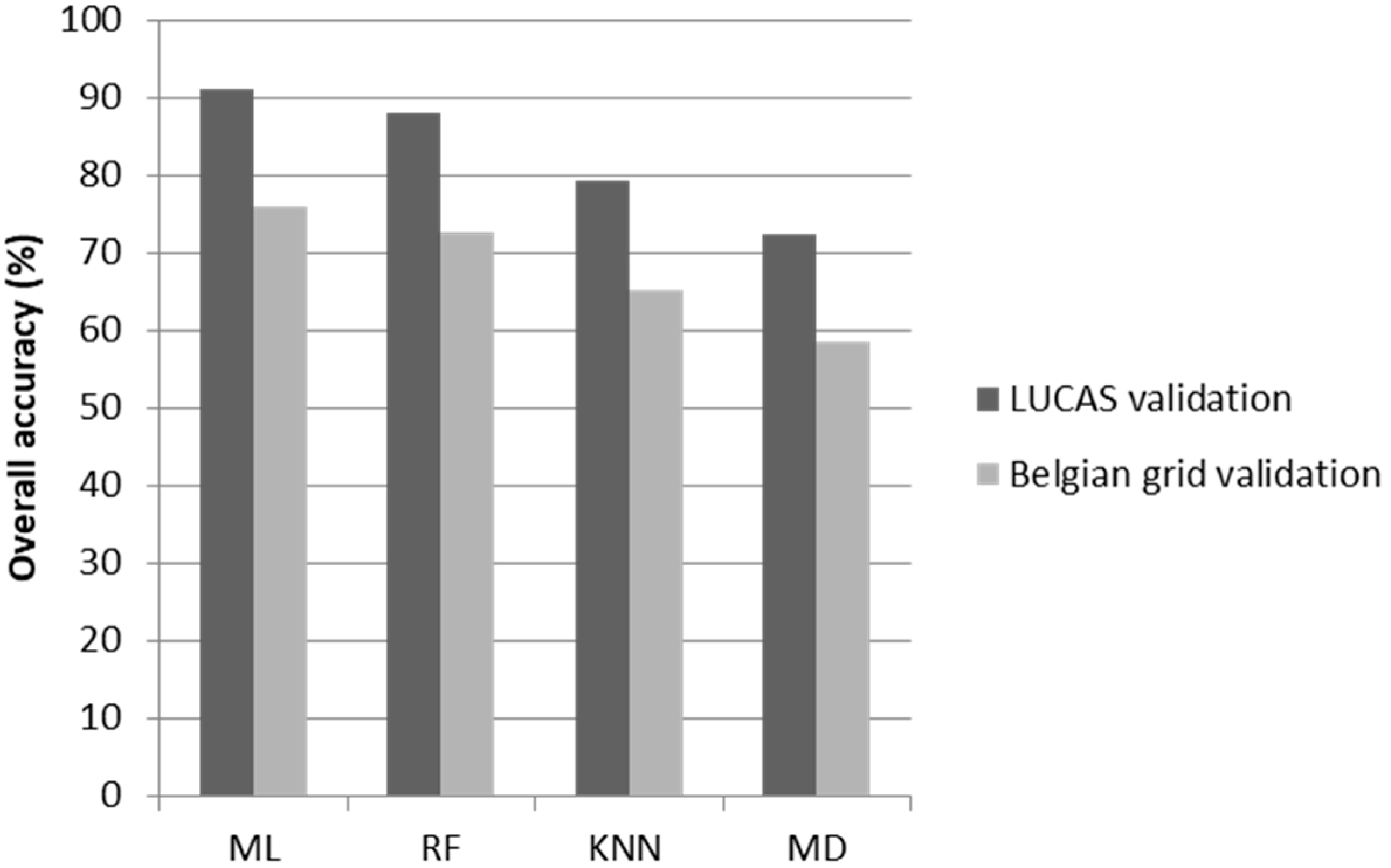
3.2. Classification Algorithms
3.3. Accuracy Assessment
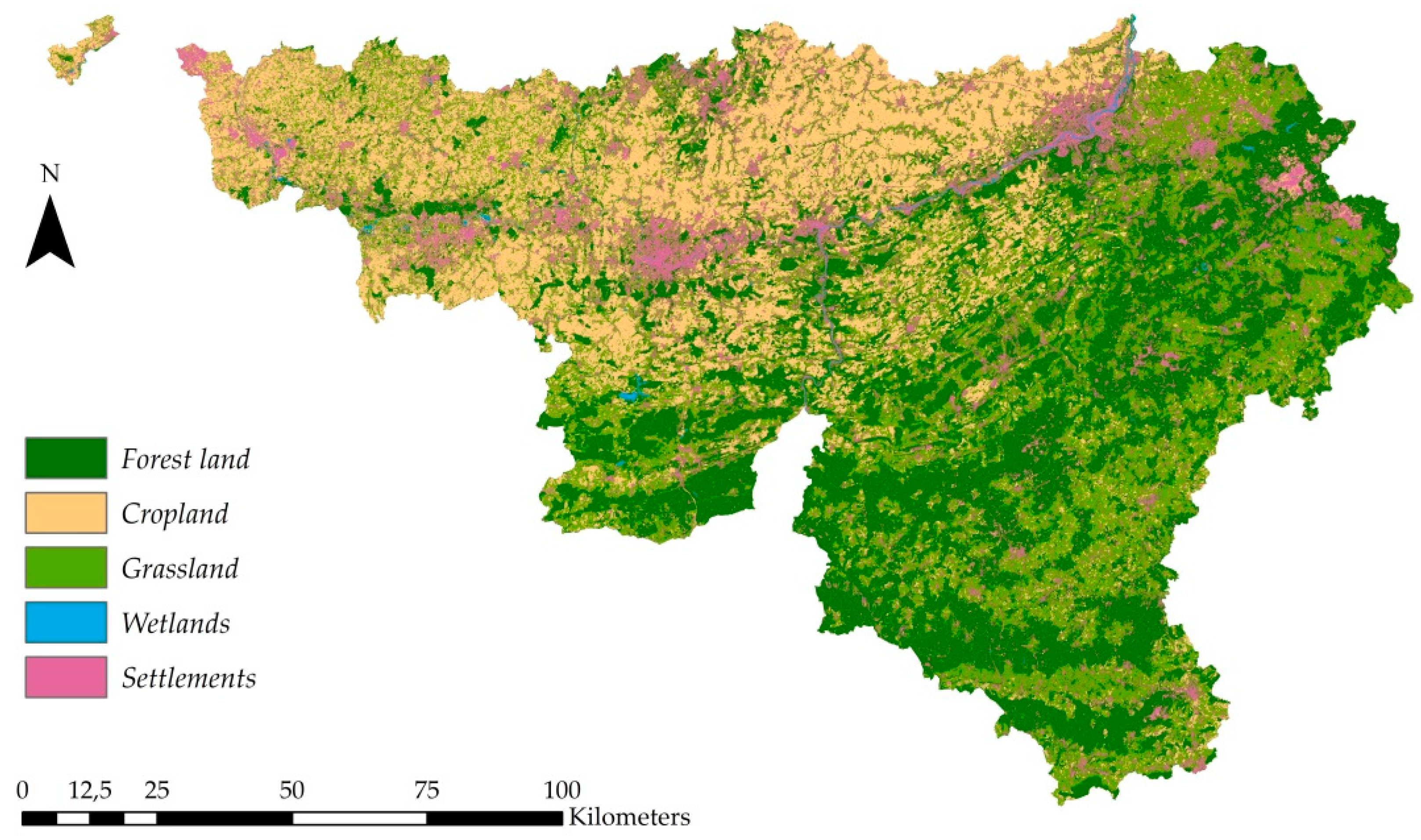
3.4. LULUCF Classification
4. Discussion
5. Conclusions
Author Contributions
Funding
Acknowledgments
Conflicts of Interest
References
- IPCC. Good Practice Guidance for Land Use, Land Use Change and Forestry; Penman, J., Gytarsky, M., Hiraishi, T., Krug, T., Kruger, D., Pipatti, R., Buendia, L., Miwa, K., Ngara, T., Tanabe, K., et al., Eds.; Institute for Global Environmental Strategies (IGES); Intergovernmental Panel on Climate Change (IPCC): Hayama, Japan, 2003; p. 632. Available online: https://www.ipcc-nggip.iges.or.jp/public/gpglulucf/gpglulucf_files/GPG_LULUCF_FULL.pdf (accessed on 3 September 2018).
- IPCC. 2006 Guidelines for National Greenhouse Gas Inventories, Prepared by the National Greenhouse Gas Inventories Programme; Eggleston, H.S., Buendia, L., Miwa, K., Ngara, T., Tanabe, K., Eds.; Institute for Global Environmental Strategies (IGES); IPCC: Hayama, Japan, 2006; Available online: https://www.ipcc-nggip.iges.or.jp/public/2006gl/vol4.html (accessed on 3 September 2018).
- Achard, F.; Grassi, G.; Herold, M.; Teobaldelli, M.; Mollicone, D. Use of Satellite Remote Sensing in LULUCF Sector; GOFC-GOLD Report No. 33; Global Observation of Forest and Land Cover Dynamics (GOFC-GOLD): Jena, Germany, 2008; p. 25. Available online: http://nofc.cfs.nrcan.gc.ca/gofc-gold/Report%20Series/GOLD_33.pdf (accessed on 15 October 2018).
- Beaumont, B.; Grippa, T.; Lennert, M.; Vanhuysse, S.; Stephenne, N.; Wolff, E. Toward an operational framework for fine-scale urban land-cover mapping in Wallonia using submeter remote sensing and ancillary vector data. J. Appl. Remote Sens. 2017, 11, 036011. [Google Scholar] [CrossRef]
- Bauwens, S.; Lejeune, P.; Herbert, J. Inventaire sur L’affectation et du Changement D’affectation des Terres et la Foresterie de la Belgique; Unpublished Report; Gembloux Agro Bio Tech: Gembloux, Belgium, 2011; p. 69. [Google Scholar]
- Blujdea, V.N.B.; Vinas, R.A.; Federici, S.; Grassi, G. The EU greenhouse gas inventory for the LULUCF sector: I. overview and comparative analysis of methods used by EU member states. Carbon Manag. 2016, 6, 247–259. [Google Scholar] [CrossRef]
- Drusch, M.; Del Bello, U.; Carlier, S.; Colin, O.; Fernandez, V.; Gascon, F.; Hoersch, B.; Isola, C.; Laberinti, P.; Martimort, P.; et al. Sentinel-2: ESA’s optical high-resolution mission for GMES operational services. Remote Sens. Environ. 2012, 120, 25–36. [Google Scholar] [CrossRef]
- Pahlevana, N.; Sarkar, S.; Franz, B.A.; Balasubramanian, S.V.; He, J. Sentinel-2 MultiSpectral Instrument (MSI) data processing for aquatic science applications: Demonstrations and validations. Remote Sens. Environ. 2017, 201, 47–56. [Google Scholar] [CrossRef]
- Liu, H.; Li, Q.; Shi, T.; Hu, S.; Wu, G.; Zhou, Q. Application of sentinel 2 MSI images to retrieve suspended particulate matter concentrations in Poyang Lake. Remote Sens. 2017, 9, 761. [Google Scholar] [CrossRef]
- Topaloglu, R.H.; Sertel, E.; Musaoglu, N. Assessment of Classification Accuracies of SENTINEL-2 and LANDSAT-8 Data for Land Cover/Use Mapping. Int. Arch. Photogramm. Remote Sens. Spat. Inf. Sci. 2016, XLI-B8, 1055–1059. [Google Scholar] [CrossRef]
- Clerici, N.; Calderón, C.A.V.; Posada, J.M. Fusion of Sentinel-1A and Sentinel-2A data for land cover mapping: A case study in the lower Magdalena region, Colombia. J. Maps 2017, 13, 718–726. [Google Scholar] [CrossRef]
- Inglada, J.; Vincent, A.; Arias, M.; Tardy, B.; Morin, D.; Rodes, I. Operational High Resolution Land Cover Map Production at the Country Scale Using Satellite Image Time Series. Remote Sens. 2017, 9, 95. [Google Scholar] [CrossRef]
- Steinhausen, M.J.; Wagnerc, P.D.; Narasimhand, B.; Waskea, B. Combining Sentinel-1 and Sentinel-2 data for improved land use and land cover mapping of monsoon regions. Int. J. Appl. Earth Obs. Geoinf. 2018, 73, 595–604. [Google Scholar] [CrossRef]
- Sola, I.; Garcia-Martin, A.; Sandonis-Pozo, L.; Alvarez-Mozos, J.; Perez-Cabello, F.; Gonzalez-Audicana, M.; Lloveria, R.M. Assessment of atmospheric correction methods for Sentinel-2 images in Mediterranean landscapes. Int. J. Appl. Earth Obs. Geoinf. 2018, 73, 63–76. [Google Scholar] [CrossRef]
- Karydas, C.G.; Gitas, I.Z.; Kuntz, S.; Minakou, C. Use of LUCAS LC Point Database for validating Country-Scale Land Cover Maps. Remote Sens. 2015, 7, 5012–5041. [Google Scholar] [CrossRef]
- Heydari, S.S.; Mountrakis, G. Effect of classifier selection, reference sample size, reference class distribution and scene heterogeneity in per-pixel classification accuracy using 26 Landsat sites. Remote Sens. Environ. 2018, 204, 648–658. [Google Scholar] [CrossRef]
- Commission Nationale Climat. Part II: Supplementary Information Required under Article 7, Paragraph 1. In National Belgian Inventory Report Submitted under the United Nations Framework Convention on Climate Change; 2016; pp. 223–240. Available online: https://unfccc.int/process-and-meetings/transparency-and-reporting/reporting-and-review-under-the-convention/greenhouse-gas-inventories-annex-i-parties/submissions/national-inventory-submissions-2016 (accessed on 1 October 2018).
- Noi, P.T.; Kappas, M. Comparison of Random Forest, k-Nearest Neighbor, and Support Vector Machine Classifiers for Land Cover Classification Using Sentinel-2 Imagery. Sensors 2017, 18, 18. [Google Scholar] [CrossRef]
- Adam, E.; Mutanga, O.; Odindi, J.; Abdel-Rahman, E.M. Land-use/cover classification in a heterogeneous coastal landscape using RapidEye imagery: Evaluating the performance of random forest and support vector machines classifiers. Int. J. Remote Sens. 2014, 35, 3440–3458. [Google Scholar] [CrossRef]
- Ghosh, A.; Joshi, P.K. A comparison of selected classification algorithms for mapping bamboo patches in lower Gangetic plains using very high resolution WorldView 2 imagery. Int. J. Appl. Earth Obs. Geoinf. 2014, 26, 298–311. [Google Scholar] [CrossRef]
- Baraldi, A.; Bruzzone, L.; Blonda, P. Quality Assessment of Classification and Cluster Maps without Ground Truth Knowledge. IEEE Trans. Geosci. Remote Sens. 2005, 43, 857–873. [Google Scholar] [CrossRef]
- Spiegel, M.R.; Stephens, L.J. Statistics, 4th ed.; McGraw-Hill: New York, NY, USA, 1961; p. 229. [Google Scholar]
- Foody, G.M. Assessing the accuracy of land cover change with imperfect ground reference data. Remote Sens. Environ. 2010, 114, 2271–2285. [Google Scholar] [CrossRef]
- Olofsson, P.; Foody, G.M.; Herold, M.; Stehman, S.V.; Woodcock, C.E.; Wulder, M.A. Good practices for estimating area and assessing accuracy of land change. Remote Sens. Environ. 2014, 148, 42–57. [Google Scholar] [CrossRef]
- Christman, Z.J.; Rogan, J. Error Propagation in Raster Data Integration -Impacts on Landscape Composition and Configuration. Photogramm. Eng. Remote Sens. 2012, 78, 617–624. [Google Scholar] [CrossRef]
- Griffith, J. The role of landscape pattern analysis in understanding concepts of land cover change. J. Geogr. Sci. 2004, 14, 3–17. [Google Scholar] [CrossRef]
- Jensen, J.R.; Cowen, D.C. Remote sensing of urban/suburban infrastructure and socio-economic attributes. Photogramm. Eng. Remote Sens. 1999, 65, 611–622. [Google Scholar] [CrossRef]


| Winter | Spring | Summer | |||
|---|---|---|---|---|---|
| T31UDS | 27 December2016 | 16 March 2016 | 1 May 2016 | 8 September 2016 | |
| T31UES | 27 December 2016 | 12 March 2016 | 8 May 2016 | 20 July 2016 | |
| T31UFS | 4 December 2016 | 1 May 2016 | 8 May 2016 | 25 September 2016 | |
| T31UGS | 4 December 2016 | 12 March 2016 | 8 May 2016 | 25 September 2016 | |
| T31UER | 7 December 2016 | 12 March 2016 | 8 May 2016 | 20 July 2016 | |
| T31UFR | 4 December 2016 | 12 March 2016 | 1 May 2016 | 8 May 2016 | 25 September 2016 |
| T31UGR | 4 December 2016 | 8 May 2016 | 8 May 2016 | 26 May 2016 | |
| T31UFQ | 4 December 2016 | 8 May 2016 | 8 May 2016 | 26 May 2016 | |
| Classifiers | OA | Error Tolerance (±) |
|---|---|---|
| MLC | 0.911 | 0.019 |
| RF | 0.880 | 0.022 |
| KNN | 0.794 | 0.027 |
| MD | 0.724 | 0.030 |
| LUCAS Validation Dataset | ||||||||
| Winter Classification (4 bands) | F | C | G | W | S | Total | User’s Accuracy (%) | |
| F | 152 | 7 | 7 | 8 | 5 | 179 | 84.9 | |
| C | 5 | 139 | 37 | 0 | 22 | 203 | 68.4 | |
| G | 12 | 20 | 146 | 3 | 11 | 192 | 76.0 | |
| W | 0 | 3 | 0 | 96 | 2 | 101 | 95.0 | |
| S | 18 | 32 | 12 | 14 | 83 | 159 | 52.2 | |
| Total | 187 | 201 | 202 | 121 | 123 | 834 | ||
| Producer’s Accuracy (%) | 81.2 | 69.1 | 72.2 | 79.3 | 67.4 | |||
| Overall Accuracy (%) | 73.86 | |||||||
| LUCAS Validation Dataset | ||||||||
| Spring Classification (4 bands) | F | C | G | W | S | Total | User’s Accuracy (%) | |
| F | 162 | 3 | 12 | 1 | 1 | 179 | 90.5 | |
| C | 6 | 127 | 59 | 0 | 11 | 203 | 62.5 | |
| G | 8 | 14 | 165 | 0 | 5 | 192 | 85.9 | |
| W | 0 | 0 | 0 | 101 | 0 | 101 | 100.0 | |
| S | 5 | 10 | 3 | 2 | 139 | 159 | 87.4 | |
| Total | 181 | 154 | 239 | 104 | 156 | 834 | ||
| Producer’s Accuracy (%) | 89.5 | 82.4 | 69.0 | 97.1 | 89.1 | |||
| Overall Accuracy (%) | 83.21 | |||||||
| LUCAS Validation Dataset | ||||||||
| Summer Classification (4 bands) | F | C | G | W | S | Total | User’s Accuracy (%) | |
| F | 171 | 1 | 4 | 1 | 2 | 179 | 95.5 | |
| C | 4 | 157 | 39 | 0 | 3 | 203 | 77.3 | |
| G | 0 | 18 | 170 | 0 | 4 | 192 | 88.5 | |
| W | 0 | 0 | 0 | 100 | 1 | 101 | 99.0 | |
| S | 0 | 6 | 9 | 2 | 142 | 159 | 89.3 | |
| Total | 175 | 182 | 222 | 103 | 152 | 834 | ||
| Producer’s Accuracy (%) | 97.7 | 86.2 | 76.5 | 97.0 | 93.4 | |||
| Overall Accuracy (%) | 88.7 | |||||||
| LUCAS Validation Dataset | ||||||||
| Winter Classification (10 bands) | F | C | G | W | S | Total | User’s Accuracy (%) | |
| F | 160 | 1 | 7 | 3 | 8 | 179 | 89.4 | |
| C | 2 | 152 | 28 | 0 | 21 | 203 | 74.9 | |
| G | 9 | 20 | 146 | 1 | 16 | 192 | 76.0 | |
| W | 2 | 0 | 3 | 90 | 6 | 101 | 89.1 | |
| S | 7 | 20 | 12 | 1 | 119 | 159 | 74.8 | |
| Total | 180 | 193 | 196 | 95 | 170 | 834 | ||
| Producer’s Accuracy (%) | 88.9 | 78.8 | 74.5 | 94.7 | 70.0 | |||
| Overall Accuracy (%) | 80.0 | |||||||
| LUCAS Validation Dataset | ||||||||
| Spring Classification (10 bands) | F | C | G | W | S | Total | User’s Accuracy (%) | |
| F | 164 | 2 | 8 | 0 | 5 | 179 | 91.6 | |
| C | 1 | 151 | 38 | 0 | 13 | 203 | 74.4 | |
| G | 10 | 12 | 156 | 0 | 14 | 192 | 81.3 | |
| W | 3 | 0 | 0 | 94 | 4 | 101 | 93.1 | |
| S | 1 | 7 | 3 | 0 | 148 | 159 | 93.1 | |
| Total | 179 | 172 | 205 | 94 | 184 | 834 | ||
| Producer’s Accuracy (%) | 91.6 | 87.8 | 76.1 | 100.0 | 80.4 | |||
| Overall Accuracy (%) | 85.5 | |||||||
| LUCAS Validation Dataset | ||||||||
| Summer Classification (10 bands) | F | C | G | W | S | Total | User’s Accuracy (%) | |
| F | 174 | 0 | 1 | 0 | 4 | 179 | 97.2 | |
| C | 1 | 182 | 12 | 0 | 8 | 203 | 89.7 | |
| G | 0 | 21 | 161 | 0 | 10 | 192 | 83.9 | |
| W | 2 | 0 | 0 | 96 | 3 | 101 | 95.0 | |
| S | 0 | 6 | 4 | 0 | 149 | 159 | 93.7 | |
| Total | 177 | 209 | 178 | 96 | 174 | 834 | ||
| Producer’s Accuracy (%) | 98.3 | 87.1 | 90.4 | 100.0 | 85.6 | |||
| Overall Accuracy (%) | 91.4 | |||||||
| LUCAS Validation Dataset | ||||||||
| Winter-Spring-Summer (4 bands) | F | C | G | W | S | Total | User’s Accuracy (%) | |
| F | 172 | 4 | 0 | 1 | 2 | 179 | 96.1 | |
| C | 1 | 184 | 17 | 0 | 1 | 203 | 90.6 | |
| G | 0 | 17 | 173 | 0 | 2 | 192 | 90.1 | |
| W | 0 | 0 | 0 | 97 | 4 | 101 | 96.0 | |
| S | 0 | 8 | 4 | 1 | 146 | 159 | 91.8 | |
| Total | 173 | 213 | 194 | 99 | 155 | 834 | ||
| Producer’s Accuracy (%) | 99.4 | 86.4 | 89.2 | 98.0 | 94.2 | |||
| Overall Accuracy (%) | 92.6 | |||||||
| LUCAS Validation Dataset | ||||||||
| Spring-Summer (4 bands) | F | C | G | W | S | Total | User’s Accuracy (%) | |
| F | 174 | 0 | 1 | 1 | 3 | 179 | 97.2 | |
| C | 1 | 175 | 23 | 0 | 4 | 203 | 86.2 | |
| G | 0 | 21 | 168 | 0 | 3 | 192 | 87.5 | |
| W | 0 | 0 | 0 | 98 | 3 | 101 | 97.0 | |
| S | 0 | 8 | 2 | 1 | 148 | 159 | 93.1 | |
| Total | 175 | 204 | 194 | 100 | 161 | 834 | ||
| Producer’s Accuracy (%) | 99.4 | 85.8 | 86.6 | 98.0 | 91.9 | |||
| Overall Accuracy (%) | 91.5 | |||||||
| LUCAS Validation Dataset | ||||||||
| Winter-Spring-Summer (10 bands) | F | C | G | W | S | Total | User’s Accuracy (%) | |
| F | 162 | 4 | 2 | 0 | 11 | 179 | 90.5 | |
| C | 1 | 182 | 12 | 0 | 8 | 203 | 89.7 | |
| G | 1 | 26 | 156 | 0 | 9 | 192 | 81.3 | |
| W | 13 | 1 | 0 | 77 | 10 | 101 | 76.2 | |
| S | 0 | 11 | 1 | 0 | 147 | 159 | 92.5 | |
| Total | 177 | 224 | 171 | 77 | 185 | 834 | ||
| Producer’s Accuracy (%) | 91.5 | 81.3 | 91.2 | 100.0 | 79.5 | |||
| Overall Accuracy (%) | 86.8 | |||||||
| LUCAS Validation Dataset | ||||||||
| Spring-Summer (10 bands) | F | C | G | W | S | Total | User’s Accuracy (%) | |
| F | 169 | 1 | 1 | 0 | 8 | 179 | 94.4 | |
| C | 1 | 188 | 10 | 0 | 4 | 203 | 92.6 | |
| G | 0 | 23 | 156 | 0 | 13 | 192 | 81.3 | |
| W | 2 | 0 | 0 | 88 | 11 | 101 | 87.1 | |
| S | 0 | 6 | 2 | 0 | 151 | 159 | 95.0 | |
| Total | 172 | 218 | 169 | 88 | 187 | 834 | ||
| Producer’s Accuracy (%) | 98.3 | 86.2 | 92.3 | 100.0 | 80.7 | |||
| Overall Accuracy (%) | 90.2 | |||||||
| Winter-Spring-Summer (4 bands) Classification | GHG Inventory Report | CLC12 | |
| Classes | kha | kha | kha |
| Forest Land | 570.91 | 556.40 | 516.74 |
| Cropland | 428.78 | 456.40 | 588.98 |
| Grassland | 464.33 | 400.40 | 321.41 |
| Wetlands | 6.32 | 16.00 | 10.10 |
| Settlements | 225.83 | 258.60 | 253.22 |
| Total | 1696.17 | 1687.80 | 1690.44 |
| Spring-Summer (4 bands) Classification | GHG Inventory Report | CLC12 | |
| Classes | kha | Kha | Kha |
| Forest Land | 570.99 | 556.40 | 516.74 |
| Cropland | 424.85 | 456.40 | 588.98 |
| Grassland | 473.91 | 400.40 | 321.41 |
| Wetlands | 7.42 | 16.00 | 10.10 |
| Settlements | 219.14 | 258.60 | 253.22 |
| Total | 1696.32 | 1687.80 | 1690.44 |
| Summer (10 bands) Classification | GHG Inventory Report | CLC12 | |
| Classes | Kha | Kha | Kha |
| Forest Land | 575.90 | 556.40 | 516.74 |
| Cropland | 451.45 | 456.40 | 588.98 |
| Grassland | 397.08 | 400.40 | 321.41 |
| Wetlands | 6.60 | 16.00 | 10,10 |
| Settlements | 265.29 | 258.60 | 253.22 |
| Total | 1696.32 | 1687.80 | 1690.44 |
© 2018 by the authors. Licensee MDPI, Basel, Switzerland. This article is an open access article distributed under the terms and conditions of the Creative Commons Attribution (CC BY) license (http://creativecommons.org/licenses/by/4.0/).
Share and Cite
Close, O.; Benjamin, B.; Petit, S.; Fripiat, X.; Hallot, E. Use of Sentinel-2 and LUCAS Database for the Inventory of Land Use, Land Use Change, and Forestry in Wallonia, Belgium. Land 2018, 7, 154. https://doi.org/10.3390/land7040154
Close O, Benjamin B, Petit S, Fripiat X, Hallot E. Use of Sentinel-2 and LUCAS Database for the Inventory of Land Use, Land Use Change, and Forestry in Wallonia, Belgium. Land. 2018; 7(4):154. https://doi.org/10.3390/land7040154
Chicago/Turabian StyleClose, Odile, Beaumont Benjamin, Sophie Petit, Xavier Fripiat, and Eric Hallot. 2018. "Use of Sentinel-2 and LUCAS Database for the Inventory of Land Use, Land Use Change, and Forestry in Wallonia, Belgium" Land 7, no. 4: 154. https://doi.org/10.3390/land7040154
APA StyleClose, O., Benjamin, B., Petit, S., Fripiat, X., & Hallot, E. (2018). Use of Sentinel-2 and LUCAS Database for the Inventory of Land Use, Land Use Change, and Forestry in Wallonia, Belgium. Land, 7(4), 154. https://doi.org/10.3390/land7040154